Robust support vector regression networks for ... - Semantic Scholar

1322

IEEE TRANSACTIONS ON NEURAL NETWORKS, VOL. 13, NO. 6, NOVEMBER 2002

Robust Support Vector Regression Networks for Function Approximation With Outliers Chen-Chia Chuang, Shun-Feng Su, Member, IEEE, Jin-Tsong Jeng, Member, IEEE, and Chih-Ching Hsiao

Abstract—Support vector regression (SVR) employs the support vector machine (SVM) to tackle problems of function approximation and regression estimation. SVR has been shown to have good robust properties against noise. When the parameters used in SVR are improperly selected, overfitting phenomena may still occur. However, the selection of various parameters is not straightforward. Besides, in SVR, outliers may also possibly be taken as support vectors. Such an inclusion of outliers in support vectors may lead to seriously overfitting phenomena. In this paper, a novel regression approach, termed as the robust support vector regression (RSVR) network, is proposed to enhance the robust capability of SVR. In the approach, traditional robust learning approaches are employed to improve the learning performance for any selected parameters. From the simulation results, our RSVR can always improve the performance of the learned systems for all cases. Besides, it can be found that even the training lasted for a long period, the testing errors would not go up. In other words, the overfitting phenomenon is indeed suppressed. Index Terms—Outliers, robust learning, support vector regression (SVR).

I. INTRODUCTION

T

HE SUPPORT vector machine (SVM) is a universal approach for solving the problems of multidimensional function estimation. Those approaches are all based on the Vapnik–Chervonenkis (VC) theory [1], [2]. Initially, it was designed to solve pattern recognition problems, where in order to find a decision rule with good generalization capability, a small subset of the training data, called the support vectors [1], [2], are selected. Experiments showed that it is easy to recognize high-dimensional identities using a small basis constructed from the selected support vectors [3]. Recently, SVM has also been applied to various fields successfully such as classification [4], [5], time prediction [6] and regression [7]–[11]. When SVM is employed to tackle the problems of function approximation and regression estimation, the approaches are often referred to as the support vector regression (SVR) [6]–[11]. The SVR type of function approximation is

Manuscript received August 26, 1999; revised December 17, 2001 and April 1, 2002. This work was supported in part by the National Science Council of Taiwan under Grant NSC 89-2218-E-009-091. C.-C. Chuang is with the Department of Electronic Engineering, Hwa-Hsia College of Technology and Commerce, Taipei 235, Taiwan, R.O.C. S.-F. Su and C.-C. Hsiao are with the Department of Electrical Engineering, National Taiwan University of Science and Technology, Taipei 106, Taiwan, R.O.C. J.-T. Jeng is with the Department of Computer Science and Information Engineering, National Huwei Institute of Technology, Huwei Jen, Yunlin 632, Taiwan, R.O.C. Digital Object Identifier 10.1109/TNN.2002.804227

very effective, especially for the case of having a high-dimensional input space. Another important advantage for using SVR in function approximation is that the number of free parameters in the function approximation scheme is equal to the number of support vectors. Such a number can be obtained by defining the width of a tolerance band. Thus, the selection of the number of free parameters can be directly related to the approximation accuracy and does not have to depend on the dimensionality of the input space or other factors as that in the cases of multilayer feedforward neural networks. In general, for any real-world applications, observations are always subject to noise or outliers. The intuitive definition of outliers is that “an observation which deviates so much from other observations as to arouse suspicions that it was generated by a different mechanism” [12]. Outliers may occur due to various reasons, such as erroneous measurements or noisy phenomenon appearing in the tail portion of some noise distribution functions. When the obtained observations contain noise or outliers, the learning process being unaware of those situations may try to fit those unwanted data and this behavior may lead to a corrupted approximation function. This phenomenon is often called overfitting [13]–[16], which usually can lead to the loss of generalization performance in the test phase. In [9], SVR has been shown to have better robust properties for various signal-to-noise ratios. In [6], SVR has also been shown to have excellent performance for both the -insensitive function and Huber’s robust function matching the correct type of noise in an application of time series prediction. Besides, a general cost function for SVR has also been proposed in considering error distributions [10], [11]. In [16], the SVM with weighted least square (LS-SVM) is proposed to overcome the effects of outliers. However, when the parameters in those approaches are not properly chosen, the final results may be affected by its parameters. This property has also been mentioned in [16]. The selection of parameters in SVR is not straightforward. In fact, for different examples, the optimal sets of parameters are also different. Thus, while facing with real problems, some methods such as -fold cross-validation, VC bounds, Xi–Alpha bound, or radius–margin bound [34], must be used to find those proper parameters. A fundamental problem of those validation approaches is that they need to use training data sets to determine whether the selected parameters are proper or not. If not, another set of parameters is tried again. First, such a trial-and-error procedure may involve extensive computation. Second, when the training data used for test contain outliers, the validation result may not be trustable. In addition, if LS-SVM or other cost functions are used, conjugate gradient methods must be used. Hence, the speed of convergence depends on

1045-9227/02$17.00 © 2002 IEEE

CHUANG et al.: ROBUST SUPPORT VECTOR REGRESSION NETWORKS

the condition numbers of matrices. This phenomenon is also mentioned in [16]. Besides, in those approaches, outliers may also possibly be taken as support vectors. We agree that good selections of the regularization constant and kernel parameters in SVR are capable of ensuring good generalization of the obtained model. However, when the regularization constant and kernel parameters are not properly selected, the resultant performances may not be good. Moreover, we are also aware of the fact that good generalization of the obtained SVR model can be ensured due to the optimization process. Nevertheless, the good generalization property comes from the use of the regularization term or the so-called weight decay term. The idea of such an approach is to minimize the values of weights during the process of minimizing errors. Such a process treats all training data equally. Even though the minimization of weights may indeed result in good generalization, the effects are different from and inferior to that of what have been traditionally used for robust learning against outliers [13], [14], [18]. Traditional robust learning is to find ways of reducing the effects of outliers. Our approach is to provide a mechanism that can facilitate such a concept. In this paper, a novel regression approach, termed as the robust SVR (RSVR) network, is proposed to enhance the robust capability of SVR. The basic idea of the approach is to adopt the concept of traditional robust statistics [22]–[24] to fine tune the model obtained by SVR. Fundamentally, the proposed network is an SVR, but equipped with a robust learning algorithm. Simulation results of the proposed approach have shown the effectiveness of the approximated function in discriminating against outliers. The remaininder of this paper is outlined as follows. Section II describes the concept of robust learning and the problems encountered in traditional robust learning algorithms. The fundamental ideas for SVR are briefly introduced in Section III. The robust properties of SVR are also discussed in the section. In Section IV, the RSVR network is proposed and its training process is introduced. Section V gives experimental results. Various loss functions were used in our simulations. Those results all showed the superiority of RSVR to the original SVR. Concluding remarks are given in Section VI. II. ROBUST LEARNING CONCEPT In neural-network applications, various robust learning algorithms that adopt robust statistics methods have been proposed to deal with outliers in the literature [14], [17]–[21]. Based on similar ideas, robust radial basis function networks [19], robust interval regression [21] and robust principal component analysis (PCA) algorithms [20], etc., have been proposed to deal with outliers existing in observations for various applications successfully. However, some problems exist in the use of those robust learning methods. A fundamental problem is how to determine the initial values of parameters. Robust learning algorithms are to discriminate against outliers in the learning process. Whether a point is considered as an outlier is determined by the estimated errors because an outlier is supposed to have a large error. Thus, those robust learning algorithms use the so-called robust cost function to discriminate against outliers

1323

from the majority by degrading the effects of those points whose estimated errors are large [22], [23]. However, the problem of such approaches is that what are desired or which points are the majorities are unknown, because the estimated errors used for identifying outliers may not be correct. Hence, when the initial weights are not properly selected, the robust cost function used in those algorithms may not correctly discriminate against those outliers. As a result, the learning process will be moving in a wrong direction and the learning performance then may become awful. The second problem in traditional robust learning networks is that the number of hidden nodes is difficult to determine [25]–[28]. With too many hidden nodes, the approximated function often interpolates all training data including noise leading to overfitting. Consequently, even though training errors can be reduced to a certain extent, generalization error, however, may become worse. On the other hand, with too few hidden nodes, the network is too simple to capture the information bearing in a complicated data set leading to underfitting. As a result, the approximated function cannot truly represent the considered function. Summarily, the selection of the number of hidden nodes is important. However, a suitable number of nodes depends not only on some available information such as the numbers of input and outputs and the number of training patterns but also on some unknown information like the type of noise and the complexity of the function to be approximated. Hence, it is not likely to select a proper number of nodes in advance. III. SVR AND ITS ROBUST PROPERTY A function approximation problem can be formulated as to , obtain a function from a set of observations, with and , where is the number of training data, is the th input vector, and is the desired output for the input . Based on the SVM theory, SVR is to approximate the given observations in an -dimensional space by a linear function in another feature space . The function in SVR is of the form (1) is an inner product defined on , is a nonlinear where to , is a weight vector to mapping function from be identified in the function, and is a threshold. Usually, the considered cost function is [31], [32] (2) where [29], [30], is the loss and the estimated function measuring the error between for a given input , and is a regular output constant. The idea of adding the regularization term is to keep the weight vector as small as possible in the approximation process. When overfitting phenomena occur, some unwanted information typically noise, has been modeled into the function.

1324


Those unwanted signals usually are not smooth, and as a consequence, some parameters may become large to accommodate such behaviors. Thus, in (2), the cost function has included the intention to minimize , which in turn, reduces the model capacity. In others words, the regularization term in (2) controls the tradeoff between the model complexity and approximation accuracy in order to ensure good generalization performance [31]. In traditional SVR, the -insensitive function is used as the loss function in (2). It was first introduced in the original SV algorithm [2], [8]. The -insensitive function is defined as for otherwise

(3)

for a previously chosen nonnegative number . The use of this loss function can lead to sparse decompositions [32] and a quadratic programming problem formulated in terms of inner products in . Note that beside of the linear term used in (3), quadratic forms and infinities are also admissible for leading to the same type of problems [32]. Other loss functions found in the literature [10] are the polynomial loss function and the “piecewise polynomial and linear” loss function. Those loss functions are listed in Table I. In our simulation, those functions are all employed in the SVR algorithm for illustration. It was shown in [2] that the solution of the above problem can be expressed in terms of support vectors, and the function is then written as

(4)

in the feature space In (4), the inner product [33]. The is usually considered as a kernel function kernel function determines the smoothness properties of solutions and should reflect a prior knowledge on data. The choice of the kernel function is usually left for users. The kernel function used in our study is Gaussian and defined as

TABLE I LOSS FUNCTIONS ARE USED IN THIS PAPER

According to the SVM theory, SVR has the advantage of self-determining its structure. Hence, there are no initialization problems for SVR. For training data sets with certain noise distributions, SVR also has shown excellent performance under the -insensitive function or Huber’s robust function [6]–[11]. However, the robust effects against training data sets with outliers are not obvious in SVR. In the SVR theory, the loss function and the parameters such as the regular constant in (2), and in the kernel function (5), must be determined in advance. The parameter in the -insensitive function, and the regular constant are powerful means for regularization and adaptation to the noise in training data [6]. Both control the network complexity and the generalization capability of SVR. However, as stated in [6], how to determining a set of proper parameters is still suboptimal and computationally extensive (if not clumsy). With different loss func, the SVR approaches may tions and/or parameter sets result in different optimum solutions under the same training data set with or without outliers. In Section V, we shall show that it is not straightforward to select those parameters properly. In [34], several validation approaches have been proposed for verifying the validation of the selected parameter set such as -fold cross-validation, VC bounds, Xi–Alpha bound, and radius–margin bound. Those approaches still suffer from various problems mentioned in Section I. In this research, instead of developing algorithms to find suitable selections for those parameters, we propose to employ traditional robust learning approaches to improve the learning performance.

(5) IV. RSVR NEURAL NETWORKS where is a constant. The coefficients s in (4) can be solved by quadratic programming methods with suitable transformation of the above problem into constraint optimization problems and properly rearranging the equation into a matrix form [7], [32]. Note that only some of s are not zeros and the corresponding vectors s are called the support vectors. In (4), the constant is unknown. Various forms can be found in the literature [9]. In our implementation, the following equation is used for [9]:

(6)

In this paper, the robust learning concept and the SVR theory are combined to form the RSVR networks. The learning of the proposed RSVR network is divided into two phases, the initial phase and the robust learning phase. The initial phase is to determine the network structure and the corresponding initial network weights through the SVR theory. When the cost function in (2) and the kernel functions in (5) are chosen, the initial weights and the structure of RSVR can be determined by the SVR theory as stated in the previous section. In this paper, the kernel function is chosen as Gaussian function. After applying the SVR theory, an initial RSVR network is obtained as

(7)


1325

where is the output of the RSVR network, is a kernel function of the SVR theory, is the number of kernel functions, which is equivalent to the number of support vectors, and is the weight vector of the network. Note that (7) can also be regarded as a classical parameterized radial basis function networks with unknown and . In the second phase, the algorithm is to adjust those weights via a robust learning approach. The robust learning algorithm is based on the algorithm proposed in [13]. It should be noted that this robust learning algorithm is employed after a period of traditional backpropagation training in [13]. This is because that approach needs a fair initial network before entering the robust learning phase. In our RSVR, SVR in fact is to replace such a procedure. There are also other similar robust learning approaches [14], [17]–[21]. An important feature of those robust learning algorithms is to use a robust cost function in the place of the quadratic form of the cost function in a standard backpropagation algorithm. is deIn the learning algorithm, a robust cost function fined as

The -estimator [13], [17], [19] is used as the robust cost function in our implementation and is defined as

(11) and are time-dependent cutoff points, and and where are constants selected as 1.73 and 0.93, respectively, as those in [19]. The influence function of (13) is obtained as

(8) is the error of where is the epoch number, is a robust cost functhe RSVR network at epoch , and tion, which directly stems from the theory of robust statistics [22], [23]. In the RSVR learning algorithms, the gradient descent method is employed and can be updated as

(9) with (10)

where is a learning constant, is usually called the influence function of the algorithm, . Note that due to the itand erative nature of the training procedure, (10) becomes for each training pattern in the implementation. We concur that the above steepest descent approach is an inferior optimization tool. However, the considered scenario is that training data set contains outliers. Traditional approaches for solving such a problem are to introduce a robust cost function [13], [14], [18], and then, a steepest descent approach is applied. The idea of such an approach is to identify outliers and then to reduce the effects of outliers directly. Other optimization tools that can directly reduce the effects of outliers are hardly found in the literature. In fact, even without the existence of outliers, the steepest descent approach can still work well in various applications of neural networks. Since our approach starts from the model constructed from SVR, which is capable of finding a nice initial network, a steepest descent approach should be enough.

(12) depends on the probabilistic distribution of The shape of and in the obtained errors [29] and on the cutoff points and basically depend on outliers. (11). Ideal values of The CUTOFF algorithm used in [13] is also adopted in our research. The CUTOFF algorithm is stated as follows. Let be an upper bound of the percentage of outliers in the training data and can be defined as follows. set, and thus , . Step 1) Compute in an increasing order and define Step 2) Sort for and . In the RSVR learning algorithm, the following inputs are required: , , 1) a set of training data , ; , , 2) a set of testing data , ; , such as Gaussian, , or 3) the kernel function B-spline; , such as the -insensitive function, 4) the loss function the quadratic function, or the “piecewise polynomial and linear” loss function; used for determining the termination 5) the threshold condition of the robust learning algorithm; 6) the maximal percentage of outliers in the training data set. is used to define the generNote that the set of testing date alization errors. The RSVR learning algorithm is summarized as follows. Step 1) Initialize the RSVR structure with the given kernel functions, the loss function, and the constant .

1326


Step 2) For each training pattern, compute the estimated result by (7) and its error. Step 3) Update the weight vector incrementally by (9) and (10). When it is in the first epoch, the robust cost funcand tion is the quadratic form by selecting large enough to count in all points. and by the Step 4) Determine the cutoff points CUTOFF algorithm. defined by (8). Step 5) Compute the robust cost function Step 6) If the termination conditions are not satisfied, then go to Step 2; otherwise, terminate the learning process.

TABLE II (a) TESTING RMSES OF SVR (IN THE UPPER PORTION) AND OF RSVR (IN THE LOWER PORTION) AFTER 1000 EPOCHS TRAINING UNDER THE "-INSENSITIVE FUNCTION WITH " 0 FOR THE sinc FUNCTION. (b) TESTING RMSES OF SVR (IN THE UPPER PORTION) AND OF RSVR (IN THE LOWER PORTION) AFTER 1000 EPOCHS’ TRAINING UNDER THE "-INSENSITIVE FUNCTION WITH " = 0:01 FOR THE sinc FUNCTION. (c) TESTING RMSES OF SVR (IN THE UPPER PORTION) AND OF RSVR (IN THE LOWER PORTION) AFTER 1000 EPOCHS’ TRAINING UNDER THE QUADRATIC FUNCTION FOR THE sinc FUNCTION. (d) TESTING RMSES OF SVR (IN THE UPPER PORTION) AND OF RSVR (IN THE LOWER PORTION) AFTER 1000 EPOCHS’ TRAINING UNDER THE “PIECEWISE POLYNOMIAL AND LINEAR LOSS FUNCTION” WITH = 0:1 FOR THE sinc FUNCTION

=

V. SIMULATION RESULTS The simulations were conducted in the Matlab environment. The SVR toolbox provided by Gunn [35] and obtained through the network service is used here. In this study, outliers are added artificially by moving some points away from designated locations. The root mean square error (RMSE) of the testing data is used to measure the performance of the learned network (generalization capability). In this study, the results of various cases with different loss functions (the -insensitive function with , the -insensitive function with , the quadratic function, and the “piecewise polynomial and linear loss function” ), different s, and different s are presented for ilwith lustration. The learning constant and the maximum percentage of outliers used in the simulation are 0.03 and 0.05, respectively. In this paper, two functions are considered. The first one is function and is defined as the

(a)

(b)

with

(13)

function is often used in the literature [7]–[11]. Fifty This are generated from the function. one training patterns in Among those data, three artificial outliers whose deviation values are 0.5, 0.4, and 0.3, respectively, are created. The other used function has also been used in [14] and [18] and is defined as with

(14)

The test data sets with 201 patterns are also generated for both examples. Note that the test data do not contain any outliers. function is first considered. The testing RMSEs of The SVR are obtained for various loss functions with different pa. Those errors are tabulated in the upper porrameter sets tion of each entry in Table II(a)–(d). The testing RMSEs of the proposed RSVR after 1000 epochs of learning are tabulated in the lower portion of each entry in Table II(a)–(d). From the re, the sults of SVR, by selecting a proper parameter set for testing RMSE of SVR can reach a nice level. It is also evident that the proposed RSVR can further improve the generalization performance of the original SVR for those cases. The average percentages of the reduced RMSEs obtained by the model constructed from SVR and from RSVR for all situations are summarized and listed in Table III.

(c)

(d)

Next, we would like to point out that SVR have different opfor different loss functions. In the timal parameter sets as the loss case of using the -insensitive function with , it has the best function [Table II(b)], when s and the testing RMSE is performance among various


1327

TABLE III AVERAGE PERCENTAGES OF THE REDUCED RMSES OBTAINED BY THE MODEL CONSTRUCTED FROM SVR AND FROM RSVR FOR THE sinc FUNCTION

TABLE IV AVERAGE PERCENTAGES OF THE REDUCED RMSES OBTAINED BY THE MODEL CONSTRUCTED FROM SVR AND FROM RSVR FOR THE FUNCTION y x

=

0.007 48. In the case of using the quadratic form [Table II(c)], , the performance is the best, and the when testing error is 0.042 19. In the case of using the “piecewise [Table II(d)], polynomial and linear loss function” with , the performance is the best and the when testing error is 0.006 58. For those cases, the proposed RSVR still can significantly improve the generalization performance. For the case of using the -insensitive function with [Table II(a)], various combinations of all can reach nice performance. It should be noted that the number of support vecis equal to the number of training data. For the tors when function, SVR is robust against training data with outliers in a broad when using the -insensitive function with . However, it is not always true range of parameter sets for other cases. is considered. In this case, varNow, the function similar ious loss functions with different parameters sets function are also used. Detailed results to those used for the are shown in [36]. From the simulations, it can found that the parameter sets for the best performance in different loss functions are different from those in the above example. For example, in as the the case of using the -insensitive function with , the performance is the loss function, when best and the testing RMSE is 0.074 37. For this case, after robust learning, the RSME becomes 0.048 46. In the case of using the , the performance is quadratic form, when the best and the testing RMSE is 0.065 45. For this case, after

(a)

(b)

=

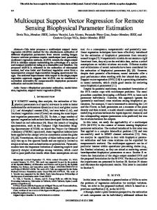
Fig. 1. (a) Obtained result of SVR using the quadratic loss function, 0:5 and C = 10 for the sinc function. In this case, all data are support vectors. (b) Obtained result of SVR using the "-insensitive function with " = 0, = 0:1 and C = 0:5 for function y = x . In this case, all data are support vectors.

robust learning, the RSME becomes 0.044 91. The average percentages of the reduced RMSEs obtained by the model constructed from SVR and from RSVR for all situations are summarized and listed in Table IV. Again, the proposed RSVR can always improve the generalization performance of SVR. Finally, we should point out that the robust performance among parameters selected in the case of using the -insensitive function with shown for the function is no longer true for this example. Two learned results are displayed in Fig. 1(a) and (b) for illustration. Fig. 1(a) is the case of using the quadratic loss funcfor the tion and the parameter sets function. Fig. 1(b) is the case of using the -insensitive function and for . It is noted with that since is zero in those shown examples, all training data are support vectors. From both figures, the approximated results appear oscillation around outliers. Such phenomena can be interpreted as the overfitting phenomenon. When the parameter sets

1328


(a)

(a)

(b)

=

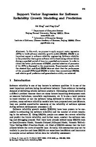
Fig. 2. (a) Obtained result of SVR using the "-insensitive function with " 0, = 3, and C = 0:5 for the sinc function. In this case, all data are support vectors. (b) Result of SVR using the "-insensitive function with " = 0, = 2 and C = 100 for function y = x . In this case, all data are support vectors.

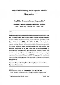
for the function and for both with the -insensitive function with , the approximated results are still affected by outliers and are shown in Fig. 2(a) and (b), respectively. These results match with the concept discussed in [15]. Therefore, it can be concluded that the selection of parameters is not straightforward. The results by RSVR after 1000 epochs based on Figs. 1(a) and (b) and 2(a) and (b) are shown in Figs. 3(a) and (b) and 4(a) and (b), respectively. It can be found that the proposed RSVR can reduce the overfitting phenomena. VI. CONCLUSION In this paper, a novel regression approach (the RSVR network) was proposed to enhance the robust capability of the SVR approaches. The basic idea of the approach is to adopt the concept of traditional robust statistics to fine-tune the function obtained by SVR. In this paper, various loss functions have been used for illustration. From our simulation results, for

(b) Fig. 3. (a) Result obtained by RSVR based on Fig. 1(a) for the sinc function. (b) Result obtained by RSVR based on Fig. 1(b) for function y = x .

some cases, the approximated results may oscillate around outliers. Such phenomena can be interpreted as the overfitting phenomenon. From the simulation examples, the selection of at the kernel function is more important than others. Different s may have different performance. However, for different examples, the optimal s are also different. In those examples, since the desired functions are exactly known, we were able to find which set of parameters can have the best performance. However, while facing with real problems, there are no ways of finding those proper parameters. Hence, we proposed to employ traditional robust learning approaches to improve the learning performance for whatever selected parameters. From the simulation results, it is evident that when improperly initial weights of the network were obtained by SVR, the improving rate of RSVR is significant. As a matter of fact, our RSVR can always improve the performance of the learned systems for all cases. Besides, it can be found that even the training lasted for a long period, the testing errors would not go up. In other word, the overfitting phenomenon is suppressed. Finally, as mentioned earlier, the number of hidden nodes in our approach can


(a)

(b) Fig. 4. (a) Result obtained by RSVR based on Fig. 2(a) for sinc function. (b) Result obtained by RSVR based on Fig. 2(b) for function y x .

=

easily be determined by the SVR theory, instead of subjective selection by heuristics in traditional neural networks. REFERENCES [1] C. Cortes and V. Vapnik, “Support vector networks,” Machine Learning, vol. 20, pp. 273–297, 1995. [2] V. Vapnik, The Nature of Statistical Learning Theory. New York: Springer-Verlag, 1995. [3] C. J. C. Burges, “A tutorial on support vector machines for pattern recognition,” Data Mining Knowledge Discovery, vol. 2, no. 2, 1996. [4] B. Schölkopf et al., “Comparing support vector machines with Gaussian kernels to radial basis function classifiers,” IEEE Trans. Signal Processing, vol. 45, pp. 2758–2765, Nov. 1997. [5] B. Boser, I. Guyon, and V. Vapnik, “A training algorithm for optimal margin classifiers,” presented at the 5th Annu. Workshop Comput. Learning Theory, 1992. [6] S. Mukherjee, E. Osuna, and F. Girosi, “Nonlinear prediction of chaotic time series using a support vector machine,” in Proc. NNSP, 1997, pp. 24–26. [7] H. Drucker et al., “Support vector regression machines,” in Neural Information Processing Systems. Cambridge, MA: MIT Press, 1997, vol. 9. [8] V. Vapnik, S. Golowich, and A. J. Smola, “Support vector method for function approximation, regression estimation, and signal processing,” in Neural Information Processing Systems. Cambridge, MA: MIT Press, 1997, vol. 9.

1329

[9] A. J. Smola and B. Schölkopf, “A tutorial on support vector regression,” Royal Holloway College, London, U.K., Neuro COLT Tech. Rep. TR-1998-030, 1998. [10] A. J. Smola, B. Schölkopf, and K. R. Müller, “General cost functions for support vector regression,” presented at the ACNN, Australian Congr. Neural Networks, 1998. [11] A. J. Smola, “Regression estimation with support vector learning machines,” Master’s thesis, Technical Univ. Munchen, Munich, Germany, 1998. [12] D. M. Hawkins, Identification of Outliers. London, U.K.: Chapman and Hall, 1980. [13] D. S. Chen and R. C. Jain, “A robust back-propagation learning algorithm for function approximation,” IEEE Trans. Neural Networks, vol. 5, pp. 467–479, May 1994. [14] C.-C. Chuang, S.-F. Su, and C.-C. Hsiao, “The annealing robust backpropagation (ARBP) learning algorithm,” IEEE Trans. Neural Networks, vol. 11, pp. 1067–1077, Sept. 2000. [15] F. E. H. Tay and L. Cao, “Application of support vector machines in financial time series forecasting,” in Int. J. Manage. Sci., 2001, pp. 309–317. [16] J. A. K. Suykens, J. De Brabanter, L. Lukas, and J. Vandewalle, “Weighted least squares support vector machines: Robustness and sparse approximation,” Neurocomput., 2001, to be published. [17] J. T. Connor, R. D. Martin, and L. E. Atlas, “Recurrent neural networks and robust time series prediction,” IEEE Trans. Neural Networks, vol. 5, pp. 240–254, Mar. 1994. [18] K. Liano, “Robust error measure for supervised neural network learning with outliers,” IEEE Trans. Neural Networks, vol. 7, pp. 246–250, Jan. 1996. [19] V. David and A. Sanchez, “Robustization of learning method for RBF networks,” Neurocomput., vol. 9, pp. 85–94, 1995. [20] C. Wang, H. C. Wu, and J. C. Principe, “A cost function for robust estimation of PCA,” Proc. SPIE, vol. 2760, pp. 120–127, 1996. [21] L. Huang, B. L. Zhang, and Q. Huang, “Robust interval regression analysis using neural network,” Fuzzy Sets Syst., pp. 337–347, 1998. [22] P. J. Rousseeuw and M. A. Leroy, Robust Regression and Outlier Detection. New York: Wiley, 1987. [23] P. J. Huber, Robust Statistics. New York: Wiley, 1981. [24] C. GriffinM. Kendall and A. Stuart, The Advanced Theory of Statistics, A. Stuart, Ed., 1977. [25] P. L. Bartlett, “For valid generalization, the size of the weights is more important than the size of the network,” in Advances in Neural Information Processing Systems, —AUTHOR, PLEASE LIST FIRST INITIALS— Mozer, Jordan, and Petshe, Eds. Cambridge, MA: MIT Press, 1997, vol. 9, pp. 134–140. [26] S. Lawrence, C. L. Giles, and A. C. Tsoi. (1996) What size neural network gives optimal generalization? Convergence properties of backpropagation. Univ. Maryland, College Park. [Online]UMIACS-TR-96-22, Tech. Rep.. Available: http://www.neci.nj.com/homepages/lawrence/papers/minima-tr96/minima-tr96.html. [27] M. Smith, Neural Networks for Statistical Modeling. New York: Van Nostrand Reinhold, 1993. [28] W. S. Sarle, “Stopped training and other remedies for overfitting,” in Proc. 27th Symp. Interface Comput. Sci. Statist., 1995, pp. 352–360. [29] V. Vapnik, Estimation of Dependences Based on Empirical Data. New York: Springer-Verlag, 1982. [30] R. O. Duda and P. E. Hart, Pattern Classification and Scene Analysis. New York: Wiley, 1973. [31] A. J. Smola and B. Schölkopf, “From regularization operators to support vector kernels,” in Neural Information Processing Systems. Cambridge, MA: MIT Press, 1997, vol. 9. , (1988) On a kernel-based method for pattern recognition, re[32] gression, approximation and operator inversion. Algorithmica [Online]. Available: http://svm.first.gmd.de/papers.html. [33] M. A. Aizerman, E. M. Braverman, and L. I. Rozonoér, “Theoretical foundations of the potential function method in pattern recognition learning,” Automat. Remote Contr., pp. 821–837, 1964. [34] K. Duan, S. S. Keerthi, and A. N. Poo, “Evaluation of simple performance measures for tuning SVM hyperparameters,” Nat. Univ. Singapore, Tech. Rep. CD-01-11, 2001. [35] S. R. Gunn. (1999) Support vector regression-Matlab toolbox. Univ. Southampton, Southampton, U.K.. [Online]. Available: http://kernel-machines.org. [36] C.-C. Chuang, “Robust modeling for function approximation under outliers,” Ph.D. dissertation, Dept. Electr. Eng., Nat. Taiwan Univ. Sci. Technol., Taipei, 2000.

1330


Chen-Chia Chuang received the B.S., M.S., and Ph.D. degrees in electrical engineering from the National Taiwan Institute of Technology, Taipei, Taiwan, R.O.C., in 1991, 1993, and 2000, respectively. He is currently an Assistant Professor in the Department of Electrical Engineering, Hwa-Hsia College of Technology and Commerce, Taipei. His current research interests are neural networks, statistics learning theory, robust learning algorithms, and signal processing.

Shun-Feng Su (S’89–M’91) received the B.S. degree in electrical engineering from National Taiwan University, Taipei, Taiwan, R.O.C., in 1983 and the M.S. and Ph.D. degrees in electrical engineering from Purdue University, West Lafayette, IN, in 1989 and 1991, respectively. He is currently a Professor in the Department of Electrical Engineering, National Taiwan University of Science and Technology, Taipei. His current research interests include neural networks, fuzzy modeling, machine learning, intelligent control, virtual reality simulation, data mining, and bioinformatics.

Jin Tsong Jeng (S’95–M’97) was born in Taiwan, R.O.C., in 1967. He received the B.S.E.E., M.S.E.E., and Ph.D. degrees all in electrical engineering from the National University of Science and Technology, Taipei, Taiwan, in 1991, 1993, and 1997, respectively. He is currently an Associate Professor in the Department of Computer Science and Information Engineering, National Huwei Institute of Technology, Huwei Jen, Yunlin, Taiwan. His primary research interests include neural networks, fuzzy systems, intelligent control, support vector regression, magnetic bearing systems, magnetic materials, nonholonomic control systems, and device drivers.

Chih-Ching Hsiao received the B.S. and M.S. degrees from the Department of Electrical Engineering, National Taiwan Institute of Technology, Taipei, Taiwan, R.O.C., in 1991 and 1993, respectively. He is currently pursuing the Ph.D. degree at the National Taiwan University of Science and Technology, Taipei. His current research interests include intelligent control and fuzzy systems.