[29] L. Wendler, T. Kraft, M. Hartung, A. Berger, A. Wixforth, M. Sundaram, J. H. English, A. C. Gossard,. Phys. Rev. B, 55, 4, 2303 (1997). [30] R.W. Wood, Phys.
Role of Wood anomalies in optical properties of thin metallic films with a bidimensional array of subwavelength holes Micha¨el SARRAZIN∗ , Jean-Pol VIGNERON∗ , Jean-Marie VIGOUREUX†
arXiv:physics/0311013v1 [physics.optics] 4 Nov 2003
∗
Laboratoire de Physique du Solide Facult´es Universitaires Notre-Dame de la Paix Rue de Bruxelles 61, B-5000 Namur, Belgium † Laboratoire de Physique Mol´eculaire, UMR-CNRS 6624 Universit´e de Franche-Comt´e F-25030 Besan¸con Cedex, France
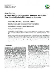
corresponds to guided modes resonances in the dielectric layer. In fact, both anomalies correspond to differents cases of the resonance effect report by A. Hessel and A.A. Oliner [19]. As shown by A. Hessel and A.A. Oliner [19], depending on the type of periodic structure the two kind of anomalies (i.e. Rayleigh’s anomalies or resonant anomalies) may occur separately or are almost superimposed. At last, we note that these concepts have been first suggested by V. U Fano [22]. In this paper we perform simulations to examine the behaviour of the optical properties of a device which consists of arrays of subwavelength cylindrical holes in a chromium layer deposited on a quartz substrate (Fig. 1). The values of permittivity being those obtained from experiments [31]. We present the key role of Rayleigh’s wavelength and eigenmodes resonances in the behaviour of the zeroth order reflexion and the transmission. Our numerical study rests on the following method. Taking into account the periodicity of the device, the permittivity is first described by a Fourier series. Then, the electromagnetic field is described by Bloch’s waves which can too be described by a Fourier series. In this context, Maxwell’s equations take the form of a matricial first order differential equation along to the z axis perpendicular to the x and y axis where the permittivity is periodic [32,33]. The heart of the method is to solve this equation. One approach deals with the propagation of the solution step by step by using the scattering matrix formalism. More explicitly, we numerically divide the grating along to the z axis into many thick layers for which we calculate the scattering matrix. The whole scattering matrix of the system is obtain by using a special combination law applied step by step to each S matrices along to the z axis. Indeed, it is well know that S matrices and their combinations are much better conditionned than transfert matrices [33]. Note that our algorithm has been compared with accuracy with others method such as FDTD or KKR [34]. In the present work the convergence is obtain from two harmonics only, i.e. for 25 vectors of the reciprocal lattice. Further more, here there is no convergence problem associated with discontinuities such that we need to use Li’s method [35,36]. In the following, for a square grating of parameter a, → − → − → note that, − g = 2π a (i e x + j e y ), such that the couple of integers (i, j) denotes the corresponding vector of the
Recents works deal with the optical transmission on arrays of subwavelength holes in a metallic layer deposited on a dielectric substrate. Making the system as realistic as possible, we perform simulations to enlighten the experimental data. This paper proposes an investigation of the optical properties related to the transmission of such devices. Numerical simulations give theoretical results in good agreement with experiment and we observe that the transmission and reflection behaviour correspond to Fano’s profile correlated with resonant response of the eigen modes coupled with nonhomogeneous diffraction orders. We thus conclude that the transmission properties observed could conceivably be explained as resulting from resonant Wood’s anomalies.
I. INTRODUCTION
Recent papers deal with optical experiments and simulations with various metallic gratings constituted of a thin metallic layer deposited on a dielectric substrate [118]. Such materials are typically one- or two-dimensional photonic crystals with a finite spatial extension in the direction perpendicular to the plane where the permittivity is periodic. One-dimensional gratings have been widelely studied in particular on account of interesting effects knows as Wood’s anomalies [19-30]. As shown by A. Hessel and A.A. Oliner [19] this effect take two distinct forms. One occurs in diffraction gratings at Rayleigh’s wavelengths if a diffracted order becomes tangent to the plane of the grating. The diffracted beam intensity increases just before the diffracted order vanishes. The other is related to a resonance effect [19]. Such resonances come from coupling between the non-homogeneous diffraction orders and the eigenmodes of the grating. Both types of anomalies may occur separately and independently, or appear together. M. Nevi`ere and D. Maystre [20,21] presented a wide study of the causes of Wood’s anomalies. In addition to the Rayleigh’s wavelengths they discovered two another possible origins of such anomalies. One, called ”plasmons anomalies”, occurs when the surface plasmons of a metallic grating are excited. The other appears when a dielectric coating is deposited on a metallic grating and 1
where εu represents either the permittivity of the vacuum (εv ), or of the dielectric substrate (εd ). We note that if ku,~g ,z becomes imaginary then diffraction orders becomes non-homogeneous. The wavelength (λ = 2πc ω ) values such that ku,~g ,z = 0 are called Rayleigh’s wavelength. We define the zeroth order transmission and reflection as, " # + 2 + 2 σ (7) k − T(0) = → N − → + X − → d, 0 2µ0 ωJv+ d 0 z d, 0
reciprocal lattice, i.e. diffraction order. Reflected and transmitted amplitudes are linked to the incident field by the use of the S scattering matrix which is calculated by solving Maxwell’s equation using a Fourier series [32]. Let us define Fscat as the scattered field, and Fin as the incident field, such that + + Nd Nv + + Xd Xv Fin = − (1) Fscat = − , Nd Nv −
Xv
−
Xd
and
where A is a vector containing all the component A− → g. The subscipts v and d are written for ”vacuum” and ”dielectric substrate” respectively, and the superscripts + and − denote the positive and negative direction along → the z axis for the field propagation. For each vector − g − of the reciprocal lattice, N −− and X are the s and p → v→ g v− g + amplitudes of the reflected field, respectively, and N − d→ g + and X − , that of the transmitted field in the device. → dg + On the same way, N +− → and X − → define the s and p pov0 v0 larizations amplitudes of the incident field, respectively. Then, Fscat is connected to Fin via the scattering matrix such as: S(λ)Fin (λ) = Fscat (λ)
R(0)
Jv−
� � σ X + 2 + 2 + kd− → Xd− → → g z Nd− g g 2µ0 ω − → g 2 ω 2 − → → g ) ×Θ(εd (ω) 2 − k // + − c
� � σ X − 2 − 2 =− kv− + X − → → g z Nv− v→ g g 2µ0 ω − → g 2 ω 2 − → → g ) ×Θ( 2 − k // + − c
S −1 (λ)Fscat (λ) = Fin (λ)
(9)
In this way, the eingenmodes of the structure are solution of eq. 9 in the case Fin (λ) = 0, i.e. S −1 (λ)Fscat (λ) = 0
(10)
This is a typical homogeneous problem, well know in the theory of gratings [20,21,36,37]. Complex wavelengths I λη = λR η +iλη , for which eq.(10) has non-trivial solutions, are the poles of det(S(λ)) as we have
(2)
det(S −1 (λη )) = 0
(11)
In this way, if we extract the singular part of S corresponding to the eigenmodes of the structure, we can write S on a analytical form as [20,21,37,38]
(4)
S(λ) =
X η
Rη + Sh (λ) λ − λη
(12)
This is a generalized Laurent series, where Rη are the residues associated which each poles λη . Sh (λ) is the holomorphic part of S which corresponds to purely nonresonant processes. Thus, assuming that f (λ) is the mth component of Fscatt (λ), we have, for the expression of f (λ) in the neighboorhood of one pole λη [20,21,37,38]
(5)
f (λ) =
where the electromagnetic field has been written as a Fourier series [32]. Θ(x) is the Heaviside function which − → gives 0 for x < 0 and +1 for x > 0. k // and ω are the wave vector component parallel to the surface, and the pulsation of an incident plane wave on the system, respectively. We also define ω ku,~g,z = (εu ( )2 − |~k// + ~g |2 )1/2 c
(8)
Moreover, numerical computation of the poles of S(λ) is important in order to study the eigenmodes of the structure. Let us write eq.8 as
Then, the flux J of the Poynting vector through a unit cell area σ, for a incident homogeneous plane wave is given by: � 2 � σ + 2 (3) + k − Jv+ = → N +− X → − → 2µ0 ω v 0 z v0 v0 Jd+ =
� � σ − 2 − 2 =− k − → N − → + X − → v0 v0 2µ0 ωJv+ v 0 z
rη + s(λ) λ − λη
(13)
where rη = [Rη Fin ]m and s(λ) = [Sh (λ)Fin ]m . II. RESULTS
The calculated transmission against the wavelength of the incident wave on the surface is shown in Fig. 2 for the
(6) 2
indeed the case, then we would expect to observe local maxima in the loss of energy. However, if we compare figure 2 with figure 4, we see that the convex regions in figure 2 are not matched by increased loss in figure 4, nevertheless the maxima of absorption seems to correspond to the minima of transmission. On the basis of these results, we investigate the role of Wood’s anomalies in the physical interpretation of our simulations. In this way, we emphazise the existence of eigenmodes and their role via resonant coupling with the electromagnetic field. First, we are stuying poles and resonances of the grating. As explained in the introduction the existence of eigenmodes is linked to the existence of poles of the scattering matrix. If we make the assumption that the role of purely non-resonant process is negligible, i.e. s(λ) ∼ 0, then eq. (13) can be approximated by the following exI pression [20,21,37,38] in the vicinity of one pole λR η + iλη
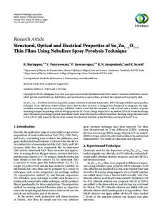
zeroth diffraction order, for light incidence normal to the surface and electric field polarized parallel to x axis. The diameter of holes (d = 500nm) and the thickness of the film (h = 100nm) have been chosen according to the experimental conditions [1,2]. The solid, and dashed lines represent the transmission for a square grating of parameter a = 1 and 1.2µm, respectively, whereas the dotted line corresponds to the transmission for a similar system without holes. In Fig. 2, it is shown that the transmission increases with the wavelength, and that it is characterized by sudden changes in the transmission marked 1 to 4 on the figure. If wavelength 1,2 and 4 correspond to minima, the wavelength 3 is nevertheless not explicitely a minimum, as we will explain it later. These values are shifted toward larger wavelengths when the grating size increases, and the minima disappear when considering a system without hole. Note that these results qualitatively agree with the experimental data of Ebbesen et al. [1,2]. Values of wavelength marked 1 to 4 are given in the first column of table 1. In the second column we give the values of the positions of maxima marked A to C on the figure. In Fig. 3 we give the calculated reflection as a function of the wavelength of the incident wave on the surface for the zeroth diffraction order, for both gratings and for the system without holes. The reflection curves are characterized by maxima (numbered 1 to 4) which correspond to the minima calculated in the transmission curves. On the same way, the location of these maxima are shifted towards larger wavelengths when the grating size increases, and they disappear when the surface is uniform. Then, it appears that the sudden decreases in transmission is correlated to an increased reflection. Moreover, the positions of the correlated maxima and minima are calculated at wavelengths which seems to correspond to Rayleigh’s wavelengths as shown in the first column of Table 2. We have reported the positions of the maxima of transmission, marked A to C, on the Fig. 3. We note that the maxima in transmission are not correlated with specifics values of reflection. In Fig. 4 we give the calculated absorption against the wavelength of the incident wave on the surface, for the zeroth diffraction order. The solid line denotes the absorption for the square grating of parameter a = 1µm, the dashed line denotes the absorption for the square grating of parameter a = 1, 2µm, and the dotted line denotes the absorption of a similar system without holes. We have reported the positions of minima in Fig. 2, numbered 1 to 4, and the positions of points A to C which denote the maxima. These peaks are found at longer wavelengths when the grating size increases, and they disappear when the surface is uniform. Thus it appears that the sudden decrease in reflectance is caused by a combination of increased reflectance and increased loss due to surface roughness. Previous work [1-18] have identified the convex regions in transmittance, i.e., those regions between the local minima, as regions where plasmons exist. If this were
|Fscat (λ)| ∼ q
|rη | �2 + λIη λ − λR η
(14) 2
which gives a typical resonance curve where the wavelength of resonance λr is equal to λR η , and where the width Γ at √12 |Fscat (λr )| is equal to 2λIη . Before searching for typical resonance in the behaviour of diffraction orders we check the existence of poles of the S matrix. In the third column in Table 2, we give the poles I λη = λR η + iλη of the S matrix computed numerically. We keep only the values whose real part is close to the values (1) to (4) in Fig. 2 and Fig. 3. This result suggests the possibility of resonant processes. In order to investigate such assumption, we have studied the behavior of the intensity of some specific diffraction orders on the vacuum/metal and substrate/metal interfaces. More precisely, we have considered the diffraction orders corresponding to the Rayleigh’s wavelengths connected to the positions of the minima obtained in the transmission curves. We compare the results with the transmission and reflection curves. In Fig. 5, curve (a) shows the modulus of the electromagnetic field of the orders (±1, 0) at the substrate/metal interface, as a function of the wavelength. The same is true for the curve (b) but the interface is now vacuum/metal. Curve (c) shows the reflected (0, 0) order. One notices the presence of localized peaks in curves (a) and (b). Simulations allow one to check that orders (±1, 0) have only p polarization. These peaks coincide with the minima of the curve of transmission of Fig. 2. Since these peaks correspond to orders with p polarization, they are probably resonances of the structure. To confirm this, we evaluate the poles by measuring the wavelength of resonance λr (which is equal to √1 |Fscat (λr )| (which is equal λR η ), and the width Γ at 2 to 2λIη ). We obtain results given in the fourth column in Table 2. One can easilly compare these results with those of the third column in table 2. This confirms the 3
profiles like those described on Fig. 7 are often called ”Fano’s profiles”. In order to refine the interpretation of our results, we represent on Fig. 8 the three curves (transmission, reflection and resonant diffraction order) on a more restricted domain of wavelength in the range 1300 − 1900 nm. In this range, since Rayleigh’s wavelength is associated to the resonant diffraction order (1, 0) for the metal/substrate interface, we represent the amplitude of this order only. The solid line denotes the transmission, the dashed line denotes the reflection and the dash-dotted line denotes the amplitude of the resonant diffraction order. We also indicate the position of the corresponding Rayleigh wavelength, as well as that of the maximum of resonance (vertical dotted lines). One labels (a) the maximum of the transmission, (b) the minimum of the reflection and (c) the maximum of the transmission. One notices that the maximum of resonance does not strictly coincide with the maximum of reflection and the minimum of transmission. Also, one notices that the maximum of reflection does not coincides with the minimum of transmission. On the other hand Rayleigh’s wavelength seems well to correspond with the minimum of transmission. We notice that the diffraction order is homogeneous for wavelengths lower than Rayleigh’s wavelength. For this reason, the resonance peak cannot be observed for wavelengths lower than Rayleigh’s wavelengths. So, if one intends to take away the position of resonance of the value of Rayleigh’s wavelength, one can make it a priori only in the direction of increasing wavelengths. Should the opposite occur, the position of the resonance peak tends towards Rayleigh’s value. As in Fig. 8, we represent on Fig. 9 the three curves (transmission, reflection and resonant diffraction order) for the same physical parameters. However, whereas in the previous case the value of the permittivity of the metal film was that of chromium [31], we use now the value equal to −25 + i1 which does not depend of the wavelength. Such value of the permittivity does not correspond to an existing material. We just choose this permittivity value for the metal such that we select a peak of resonance farther from Rayleigh’s wavelength than in the previous case. The choice of this value only comes from the research of the compromise between the position from the peak of resonance and its width so as to illustrate our matter clearly. As in Fig. 8, (a) is the maximum of the transmission, (b) the minimum of the reflection and (c) the maximum of the transmission. One names (d) the minimum of the transmission. This time, one notices in a clear way the absence of coincidence between the peak of resonance and the minima (respectively the maxima) of reflection (respectively of transmission). Contrary to what is generally assumed [1-16], one sees that the nonresonant Wood’s anomalies connected to Rayleigh’s wavelengths are not the cause of the minima of transmission. They simply correspond to a discontinuity of each of the three curves. It is particularly important to note that the profiles of the trans-
resonant characteristic of the diffraction orders (±1, 0) at the metal/vacuum and metal/substrate interfaces (A. Hessel and A.A. Oliner has called such diffraction orders ”resonant diffraction orders” [19]). Note that the orders (±1, 0) at the vacuum/metal interface and (±1, ±1) at the substrate/metal interface has poles with closer real part. This means that both modes are almost degenerated with the consequence that both modes effects can’t be clearly distinguished particularly for the transmission. So, the wavelength (3) does not seem to provide a minimum as clearly as the wavelength (2). Fig. 6 shows the behavior of the amplitude modulus of the diffraction orders (0, ±1) for the vacuum/metal (curve (a)) and for the substrate/metal (curve (b)) interfaces, respectively, as a function of the wavelength. Curve (c) corresponds to the order (0, 0) in transmission. All these orders exist only with a polarization s. One notices that the minima of these curves are correlated with the peaks of resonances. On the other hand, we know that orders with s polarization cannot present resonances. From this point of view, the minima of the curve of transmission of the Fig. 2 are correlated with the resonances, while the behavior of the convex parts of the curves of transmission can be interpreted according to the profile of the orders of polarization p. Let us now turn to Wood’s anomalies. We consider the case where purely non-resonant process can’t be totaly neglected such that we suppose s(λ) ∼ s0 . Thus, it is easy to show that eq.(13) can be written as [19,22] 2
|Fscat (λ)| =
λ − λR z
+ λIz
2
+ λIη
2
2
(15)
and λIz = λIη − ν I
(16)
λ − λR η
with R R λR z = λη − ν
�2
�2
|s0 |
where ν=
rη s
(17)
Coefficient ν shows the significance of resonant effect compared with purely non-resonant effects. λz = λR z + iλIz corresponds to the zero of eq. (13) and (15). Eq. (15) corresponds to the profiles of Fig. 7. This last expression takes into account the interferences between resonant and purely non-resonant processes. In this way, the profiles which correspond to the eq. (14), i.e. a purely resonant process, tend to become asymmetric. As shown in Fig. 7, dashed curve shows a typically resonant process like those described by eq.(14). On the other hand, solid and dash-dotted curves show a typical behaviour where a minimum is followed by a maximum, and vice versa as2 suming the values of ν. These profiles tend to |s0 | when λ tends to ±∞. We note that these properties, which result from the interference of resonant and non-resonant processes, are similare to those described by A.A. Hessel, A. Oliner [19] and V.U. Fano [22]. For this reason the 4
In other words, the minimum (d) in Fig. 8 comes from the cut off and the discontinuity introduce between the minimum and the maximum of the Fano’s profile at the Rayleigh’s wavelength. On the other hand, note that maximum (a) of the transmission and maximum (c) of the reflection just localized rests after Rayleigh’s wavelength. For the reflection, minima (b) tends to be shifted towards low wavelength. Previous works [1-16] have identified the convex regions in transmission, i.e., the regions between the minima, as regions where plasmons exist. The present study tends to qualify this hypothesis, since it shows that the experimental results can be described in terms of Wood’s anomalies. Indeed, as shown by V.U. Fano [22], A. Hessel and A.A. Oliner [19], for one dimensionnal gratings, Wood’s anomalies can be treated in terms of eigenmodes grating excitation. In this context, these authors demonstrated the asymmetric behavior of the intensities of the homogeneous diffraction orders according to the wavelength. One can conclude that the results of T.W. Ebbesen’s experiments correspond to the observation of resonant Wood’s anomalies. Here, as we use metal in our device, it seems natural to assume that these resonances are surface plasmons resonances. Nevertheless, it is important to note that our analysis don’t make any hypothesis on the origin of the eigenmodes. This involve that it could be possible to obtain transmission curves similar to those for metals, by substituted the surface plasmons by polaritons or guided modes. This work is in progress.
mission and the reflection correspond to Fano’s profiles as discussed below. One can interpret the behavior of these spectra in term of resonant Wood’s anomalies in the sense described by V. U. Fano [22] and by A. Hessel and A.A. Oliner [19]. III. DISCUSSION
In order to understand the physical mechanisms responsible for the behavior observed on Fig. 8 and Fig. 9, we have represented in Fig. 10 the corresponding involved processes. On Fig. 10, circles A and B represent diffracting elements (e.g. holes). So, an incident homogeneous wave (i) diffracts in A and generates a nonhomogeneous resonant diffraction order (e) (e.g. (1, 0)). Such order is coupled with a eigenmode which is characterized by a complex wavelength λη . It becomes possible to excite this eigenmode which leads to a feedback reaction on the order (e). This process is related to the resonant term. The diffraction order (e) diffracts in B and generates a contribution to the homogenous zero diffraction order (0, 0). Thus, one can ideally expect to observe a resonant profile, i.e. lorentzian like, for the homogenous zero diffraction order (0, 0) which appears in B. Nevertheless, it is necessary to account for nonresonant diffraction processes related to the holomorphic term. So, incident wave (i), here represented in B, generates a homogeneous zero order. Then, one takes into account the interference of two rates, resonant and non resonant contribution to zero order. The resulting lineshapes are typically the Fano’s profiles which correspond to resonant process where one takes into account nonresonant effects. One notes that a maximum in transmission does not necessary correspond to the maximum of resonance of a diffraction order. It is exactly the process observed on Fig. 9 where the resonance is associated with the diffraction order (1, 0). So, the Fano’s profiles of the reflection and the transmission, result from the superimposing of resonant and nonresonant contribution to the zero diffraction order. If one refers to Fig. 8, the concrete case of the chromium, the resonance is closer to Rayleigh’s wavelength than in the case of the Fig. 9. In another hand the positions of the maximum and the minimum of a Fano’s profile are determined by the resonance position. More precisely, if the resonance is shifted in a given direction, the maximum and the minimum of the Fano’s profile tends to be shifted in the same way. Consequently, in the present case, the maximum and the minimum of the asymmetric Fano’s profile is shifted toward Rayleigh’s wavelength in the same way as the resonant response. In Fig. 8, in the case of the transmission, minimum (d) is not of the same kind of the minimum (d) in Fig. 9. This is not a true minima of the Fano’s profile. All occurs like if the minimum of the Fano’s profile disappears behind the Rayleigh’s wavelength towards low wavelength.
IV. CONCLUSION
Using a system similar to that used in recent papers [1,2], we have shown that numerical simulations give theoretical results in good qualitative agreement with experiments. Previous authors have suggested that the results are due to the presence of the metallic layer, such that the surface plasmons could give rise to transmission curves of these characteristics. We have performed simulations using the same geometry, and we have observed that the transmission and reflection behaviour correspond to Fano’s profiles correlated with resonant response of the eigenmodes coupled with nonhomogeneous diffraction orders. We thus conclude that the transmission properties observed could conceivably be explained as resulting from resonant Wood’s anomalies. [1] T.W. Ebbesen, H.J. Lezec, H.F. Ghaemi, T. Thio, P.A. Wolff, Nature (London) 391, 667 (1998) [2] T. Thio, H.F. Ghaemi, H.J. Lezec, P.A. Wolff, T.W. Ebbesen, JOSA B, 16, 1743 (1999) [3] H.F. Ghaemi, T. Thio, D.E. Grupp, T.W. Ebbesen, H.J. Lezec, Phys. Rev. B, 58, 6779 (1998) [4] U. Schr¨oter, D. Heitmann, Phys. Rev. B, 58, 15419 (1998)
5
[5] D. E. Grupp, H.J. Lezec, T. Thio, T.W. Ebbesen, Adv. Mater, 11, 860 (1999) [6] T.J. Kim, T. Thio, T.W. Ebbesen, D.E. Grupp, H.J. Lezec, Opt. Lett, 24, 256 (1999) [7] J.A. Porto, F.J. Garcia-Vidal, J.B. Pendry, Phys. Rev. Lett., 83, 2845 (1999) [8] Y. M. Strelniker, D. J. Bergman, Phys. Rev. B, 59, 12763, (1999) [9] S. Astilean, Ph. Lalanne, M. Palamaru, Optics Comm. 175 (2000) 265-273 [10] D.E. Grupp, H.J. Lezec, T.W. Ebbesen, K.M. Pellerin, T. Thio, Applied Physics Letters 77 (11) 1569 (2000) [11] E. Popov, M. Nevi`ere, S. Enoch, R. Reinisch, Phys. Rev. B, 62, 16100 (2000) [12] W.-C. Tan, T.W. Preist, R.J. Sambles, Phys. Rev. B 62 (16) 11134 (2000) [13] T. Thio, H.J. Lezec, T.W. Ebbesen, Physica B 279 (2000) 90-93 [14] A. Krishnan, T. Thio, T. J. Kim, H. J. Lezec, T. W. Ebbesen, P.A. Wolff, J. Pendry, L. Martin-Moreno, F. J. Garcia-Vidal, Optics Comm., 200, 1-7 (2001) [15] L. Martin-Moreno, F.J. Garcia-Vidal, H.J. Lezec, K.M. Pellerin, T. Thio, J.B. Pendry, T.W. Ebbesen, Phys. Rev. Lett., 86, 1114 (2001) [16] L. Salomon, F. Grillot, A.V. Zayats, F. de Fornel, Phys. Rev. Lett., 86 (6), 1110 (2001) [17] M.M.J. Treacy, Appl. Phys. Lett., 75, 606, (1999) [18] J.-M. Vigoureux, Optics Comm., 198, 4-6, 257 (2001) [19] A. Hessel, A. A. Oliner, Applied Optics 4 (10) 1275 (1965) [20] D. Maystre, M. Nevi`ere, J. Optics, 8, 165 (1977) [21] M. Nevi`ere, D. Maystre, P. Vincent, J. Optics, 8, 231 (1977) [22] V.U. Fano, Ann. Phys. 32, 393 (1938) [23] R. H. Bjork, A. S. Karakashian, Y. Y. Teng, Phys. Rev. B, 9, 4, 1394 (1974) [24] P.J. Bliek, L.C. Botten, R. Deleuil, R.C. Mc Phedran, D. Maystre, IEEE Trans. Microwave Theory and Techniques, MTT-28 1119-1125 (1980) [25] D. Deaglehole, Phys. Rev. Lett., 22, 14, 708 (1969) [26] E. Popov, L. Tsonev, D. Maystre, Applied Optics 33 (22) 5214 (1994) [27] Lord Rayleigh, Proc. Roy. Soc. (London) A79, 399 (1907) [28] K. Utagawa, JOSA 69 (2) 333 (1979) [29] L. Wendler, T. Kraft, M. Hartung, A. Berger, A. Wixforth, M. Sundaram, J. H. English, A. C. Gossard, Phys. Rev. B, 55, 4, 2303 (1997) [30] R.W. Wood, Phys. Rev. 48, 928 (1935) [31] D.W. Lynch, W.R. Hunter, in Handbook of Optical Constants of Solids II, E.D. Palik, (Academic Press, Inc., 1991) [32] J.P. Vigneron, F. Forati, D. Andr´e, A. Castiaux, I. Derycke, A. Dereux, Ultramicroscopy, 61, 21 (1995)
[33] J.B. Pendry, P.M. Bell, NATO ASI Series E Vol. 315 (1995) [34] V. Lousse, K. Ohtaka, Private Communication (2001) [35] L. Li, JOSA A 13 (9) 1870 (1996) [36] L. Li, JOSA A 14 2758 (1997) [37] E. Centeno, D. Felbacq, Phys. Rev. B 62 (12) R7683 (2000) [38] E. Centeno, D. Felbacq, Phys. Rev. B 62 (15) 10101 (2000) [39] R. Petit, Electromagnetic Theory of Gratings, Topics in current Physics, 22, Springer Verlag (1980)
V. CAPTIONS
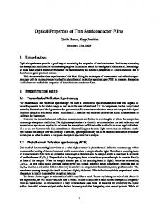
FIG. 1 Diagrammatic view of the system under study. Transmission and reflection are calculated for the zeroth order and at normal incidence as in experiments. FIG. 2 Percentage transmission of the incident wave against its wavelength on the surface, for the zeroth diffraction order. The solid line denotes the transmission for the square grating of parameter a = 1µm, the dashed line denotes the transmission for the square grating of parameter a = 1.2µm, and the dotted line denotes the transmission of a similar system without holes. The points numbered 1 to 4 denote sudden changes in the transmission whereas the points A to C denote the maxima. FIG. 3 Reflection against the wavelength of the incident wave on the surface, for the zeroth diffraction order. The solid line denotes the reflection for the square grating of parameter a = 1µm, the dashed line denotes the reflection for the square grating of parameter a = 1, 2µm, and the dotted line denotes the reflection of a similar system without holes. We note that the minima in Fig. 2 are matched by peaks in the reflection (see the previous figure), numbered 1 to 4. We have reported the points A to C which denote the positions of maxima of the transmission. FIG. 4 Absorption against the wavelength of the incident wave on the surface, for the zeroth diffraction order. The solid line denotes the absorption for the square grating of parameter a = 1µm, the dashed line denotes the absorption for the square grating of parameter a = 1, 2µm, and the dotted line denotes the absorption of a similar system without holes. We have reported the positions of minima in Fig. 2, numbered 1 to 4, and the positions of points A to C which denote the maxima. FIG. 5 Curve (a) shows the modulus of the electromagnetic field of the orders (±1, 0) at the substrate/metal interface, as a function of the wavelength. Idem for the curve (b) but for the vacuum/metal interface. Curve (c) shows the reflected (0, 0) order. One notices the presence of localized peaks in curves (a) and (b). The amplitude of the incident field is equal to 1 V.m−1 .
6
FIG. 6 Behavior of the amplitude modulus of the diffraction orders (0, ±1) respectively for the interface vacuum/metal (curve (a)) and for the interface substrate/metal (curve (b)) as a function of the wavelength. Curve (c) corresponds to the order (0, 0) in transmission. All these orders exist only with a polarization s. The amplitude of the incident field is equal to 1 V.m−1 . FIG. 7 Some examples of typical Fano’s profiles. FIG. 8 The set of three curves (transmission, reflection and resonant diffraction order) on a more restricted domain of wavelength included between 1300 nm and on 1900 nm. In this domain Rayleigh’s wavelength is associated to diffraction order (1, 0) for the interface metal/substrate. We also indicate the position of the wavelength of corresponding Rayleigh as well as that of the maximum of resonance. One names (a) the maximum of the transmission, (b) the minimum of the reflection and (c) the maximum of the reflection. Solid line : transmission, dashed line : reflection, dash-dotted line : resonant diffraction order. The amplitude of the incident field is equal to 1 V.m−1 . FIG. 9 Similar system than in Fig. 7 except for the value of the permittivity of the metal film here equal to −25 + i1. As in Fig. 7, (a) is the maximum of the transmission, (b) the minimum of the reflection and (c) the maximum of the reflection. One names (d) the minimum of the transmission. The amplitude of the incident field is equal to 1 V.m−1 . FIG. 10 Diagrammatic representation of the processes responsible of the behaviour of the transmission properties. TABLE 1 : Positions of minima and maxima of transmission. TABLE 2 : Comparison between Rayleigh’s wavelengths (second column) of some diffraction orders (first column) with the poles of the scattering matrix computed numerically (third column) and evaluated by measuring the wavelength of resonance λr , and the width Γ of some resonance curves (fourth column). (v/m) and (s/m) denote vacuum/metal interface and substrate/metal interface respectively.
7
z
�
�������� ��� � � ���� ����� ������� ��� �
����������
�� � ����� �
�� ����
6 B
Transmission (%)
5
4
4
C
3 2
3 1 2
A
1
0 500
750
1000
1250
1500
Wavelength (nm)
1750
2000
Diffraction
Rayleigh's
Poles (nm)
Extrapolated
Order
Wavelength (nm)
( 1 , 1 ) v/m
707.1
717.75 + i20
711.86 + i19.21
( 1 , 0 ) v/m
1000
1010 + i27
1013.26 + i25.12
( 1 , 1 ) s/m
1025.37
1010.25 + i59
1042.81 + i56.14
( 1 , 0 ) s/m
1445.29
1438.75 + i54
1462.41 + i71
Poles (nm)
75 70
Reflection (%)
65 60 55 50 4
45 3 A
40
1
C
B
2
35 500
750
1000
1250
1500
Wavelength (nm)
1750
2000
55 1
Absorption (%)
3 2
50
B
4
C
45 A
40
35
30
25 500
750
1000
1250
1500
Wavelength (nm)
1750
2000
1.0
Amplitude (V.m-1)
0.8
(c)
0.6
0.4
(b) (a)
0.2
0.0 400
600
800
1000
1200
1400
1600
Wavelength (nm)
1800
2000
0.22 (c)
Amplitude (V.m-1)
0.20 0.18 0.16 0.14 0.12 0.10
(a)
0.08 (b) 0.06 0.04 400
600
800
1000
1200
1400
1600
Wavelength (nm)
1800
2000
Amplitude
λR
Wavelength
12 (c)
10
10 (b)
8
8
6
6
4
2 1300
4
(a) (d)
λR
1400
1500
1600
1700
Wavelength (nm)
1800
2 1900
Amplitude (V.m-1)
Reflection and Transmission (%)
12
2.0
λ
R
1.5
1.5
(c)
-1 Amplitude (V.m )
Reflection and Transmission (%)
2.0
(a)
1.0
0.5
(d)
1.0
0.5
(b)
0.0
0.0 1200
1400
1600
1800
Wavelength (nm)
2000
� ������ �� �� ��� ���� � � � � ���� � ��������� ���� � �������
�����
����� � �
η
λ λη
�
��� i
�� ��� ��������
i
sλ
Minima (nm)
Maxima (nm)
( 1 ) 708.90
( A ) 951.21
( 2 ) 1001.44
( B ) 1320.57
( 4 ) 1447.64
( C ) 1678.12