1
Saliency Detection with Spaces of Background-based Distribution
arXiv:1603.05335v1 [cs.CV] 17 Mar 2016
Tong Zhao, Lin Li, Xinghao Ding, Yue Huang and Delu Zeng*
Abstract—In this letter, an effective image saliency detection method is proposed by constructing some novel spaces to model the background and redefine the distance of the salient patches away from the background. Concretely, given the backgroundness prior, eigendecomposition is utilized to create four spaces of background-based distribution (SBD) to model the background, in which a more appropriate metric (Mahalanobis distance) is quoted to delicately measure the saliency of every image patch away from the background. After that, a coarse saliency map is obtained by integrating the four adjusted Mahalanobis distance maps, each of which is formed by the distances between all the patches and background in the corresponding SBD. To be more discriminative, the coarse saliency map is further enhanced into the posterior probability map within Bayesian perspective. Finally, the final saliency map is generated by properly refining the posterior probability map with geodesic distance. Experimental results on two usual datasets show that the proposed method is effective compared with the state-of-theart algorithms. Index Terms—Saliency detection, eigendecomposition, backgroundness prior, Mahalanobis distance.
I. I NTRODUCTION S a subfield of computer vision and pattern recognition, image saliency detection is an interesting and challenging problem which touches upon the knowledge from multiple subjects like mathematics, biology, neurology, computer science and so on. Many previous works have demonstrated that saliency detection is significant in many fields including image segmentation [1], objection detection and recognition [2], image quality assessment [3], image editing and manipulating [4], visual tracking [5], etc. The models of saliency detection can be roughly categorized into bottom-up and top-down approaches [6], [7]. In this work, we focus on bottom-up saliency models. In recent years, color contrast cue [8], [9] and color spatial distribution cue [10] are widely used in saliency detection. It is considered that salient objects always show large contrast over their surroundings and are generally more compact in the image domain. Saliency algorithms based on these two cues usually work well when the salient object can be distinctive in terms
A
Accepted by IEEE Signal Processing Letters in Mar. 2016. D. Zeng, T. Zhao, L. Li, Y. Huang and X. Ding are with School of Information Science and Engineering, Xiamen University, China. This work was supported in part by the National Natural Science Foundation of China under Grants 61103121, 61172179, 81301278, 61571382 and 61571005, in part by the Fundamental Research Funds for the Central Universities under Grants 20720160075, 20720150169 and 20720150093, in part by the Natural Science Foundation of Guangdong Province of China under Grants 2015A030313589 and by the Research Fund for the Doctoral Program of Higher Education under Grant 20120121120043. *Corresponding to:
[email protected] for Delu Zeng.
of contrast and diversity, but they usually fail in processing images containing complicated background which involves various patterns. On the other hand, pattern distinctness is described in [11] by studying the inner statistics (actually corresponds to the distribution for the feature) of the patches in PCA space. This method achieves favorable results but there still exists some background patterns which are misjudged to be salient. In addition, by assuming most of the narrow border of the image be the background region, backgroundness prior plays an important role in calculating the saliency maps in many approaches [12], [13], [14]. However, if the patches on the border are treated as background patches directly, these algorithms often perform inadequately when the potential salient objects touch the image border. Based on the above analysis, we propose a saliency detection method considering the following aspects which also go to our contributions: 1) We combine the backgroundness prior into constructing the spaces of background-based distribution implicitly (not directly) to investigate the background, where we will find Euclidean and l1 metrics may not be suitable in exploring the distribution (inner statistics) for the patches and we should quote some other metric to describe the patch difference appropriately. 2) In the step of refinement, we also design a new up-sampling scheme based on geodesic distance. II. P ROPOSED ALGORITHM Here we describe the proposed approach in three main steps. Firstly, the patches from image border are used to generate a group of spaces of background-based distribution (SBD) to compute the coarse saliency map. Secondly, in the Bayesian perspective, the coarse saliency map is enhanced. Then the final saliency map is obtained by using a novel up-sampling method based on geodesic distance. And the main framework is depicted in Fig. 1. A. Spaces of background-based distribution The work [11] suggests that a pixel be salient if the patch containing this pixel has less contribution to the distribution of the whole image treated in PCA system. However, problem may occur when the area of the salient object is overwhelming in size. In this case, if all the image patches are utilized to do PCA, the patches in the salient object may have high contribution to distribution of the whole image patches, then naturally the difference between the salient patches and the whole image will not be discriminative. In order to increase this difference and make the salient object be much discriminative from the background, in this paper we aim to re-establish
2
(a) (b) (c) (d) (e) Fig. 1: Main framework of the proposed approach. (a) Input image. (b) Coarse saliency map based on SBD. (c) Posterior probability map based on Bayesian perspective. (d) Refinement. (e) Ground-truth.
the background distribution in some new spaces, called spaces of background-based distribution (SBD). For this purpose, we have the following considerations: 1) Feature representation For the patches, color information is used to represent their features. Particularly, two color spaces are used here, including CIE-Lab and I-RG-BY. CIE-Lab is most widely used in previous works, while I-RGBY that is transformed from RGB color space is also proved to be effective in saliency detection algorithm [15], where denotes the intensity channel, RG = R − G I = R+G+B 3 and BY = B − R+G are two color channels. Thus, if we take 2 a 7 × 7 patch as an example, the feature of this patch will be represented by a 294 × 1 column vector (6 × 7 × 7 = 294). And here we denote this vectorized feature for image patch i to be f (i). 2) Background patches selection We define the pseudobackground region as the border region of the image like the work in [16]. To improve the performance, some approaches [13], [17] divide the patches on image border into four groups including top, bottom, left and right, and deal with them respectively. In our method, we do not simply consider some certain border in a single direction, but consider the correlations between every two neighboring connective borders. This is considered to be more reasonable since the neighboring connective borders tend to present similar background information. As a result, we get four groups of patches that are located around the image border. Particularly, these S 4 groups are denoted as {G } , where G = B B , G q 1 t l 2 = q=1 S S S Bt Br , G3 = Bb Bl , G4 = Bb Br , and Bt , Bb , Bl , Br are the sets of vectorized patches on the top, bottom, left and right borders of the image respectively. To clearly present the proposed idea in the view of metric space, we choose to start with eigendecomposition. Particularly, with eigendecomposition we have Uq and Λq to denote the matrices of eigenvectors and eigenvalues of the covariance matrices Cq for Gq , q = 1, · · · , 4, respectively. With Uq , for each patch i, we have tq (i) = UqT f (i), q = 1, · · · , 4
(1)
where tq (i) will be the element (new coordinates) of patch i in the q-th SBA. Then, we turn to introduce some appropriate metric for these elements. Considering the fact that the construction of these elements is carried out on the suspicious background patches, it is speculated that a patch which is similar to the background should be highly probable in the distribution while a patch belongs to the salient region should be highly probable away from the distribution. So, the metric needs to be carefully designed. l1 metric is utilized in [11] to calculate the patch
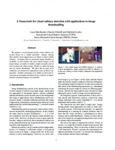
Fig. 2: The comparison of three metrics to show that Mahalanobis distance is more appropriate than Euclidean metric or l1 metric. The figure shows the distribution of patches of a tested image whose principal components are marked by the orange solid lines. Compared with p2 , p1 is less probable in the background distribution and hence should be considered more distinct, while p2 is more probable in the background distribution and hence should not be considered distinct. However, the level lines of l1 metric (green dashdotted line c2 ) and the Euclidean metric (purple dotted line c3 ) reveal the same distance between the two patches to the average patch po . The level lines of Mahalanobis distance (black dashed line c1 and c4 ) show that p1 is further away than p2 w.r.t po .
distinctness in its PCA coordinate systems and is proved to be more effective than Euclidean metric. However, it may become invalid in our spaces if one ignores the distribution of the data. In this case, Mahalanobis distance [18], [19] is used here instead exactly for the elements obtained above, and its effectiveness is explained in detail in Fig. 2. Therefore, for each patch i we compute a distance dq (i) as its Mahalanobis distance via −1
dq (i) = kΛq 2 (tq (i) − poq )k2 , q = 1, · · · , 4
(2)
where Λq is the matrix of eigenvalues and poq is in the transformed space projected from the average patch fqo for Gq . It is reasonable to understand that Λq used here is to denote the influence of different scales in different components of the eigenvectors from Uq (Fig. 2) and it is better to describe the distribution of the patches with this metric. In fact, though the −1 distance can be directly computed by kCq 2 (f (i) − fqo )k2 , the two ways of definition of Mahalanobis distance are equivalent, and it is more convenient to elaborate the proposed idea by the above context of eigendecomposition. To suppress the value of dq from the background as much as possible while retaining the one in the salient regions, we set a threshold H to update dq , i.e., if dq (i) < H, dq (i) = 0, where H is set to be the average value of dq computed by Eq.(2). The reason we do this thresholding is originated from the fact that more than 95 percent of images have larger background area than the salient area when investigating a widely used datasets MSRA5000 [20]. So for each group Gq , after repeating the calculations from Eq.(1) to Eq.(2), we get four adjusted Mahalanobis distance maps that labeled as {Sqth }4q=1 . Each map is normalized to [0,1]. Next, we create the single-scale coarse saliency map S cs by taking a weighted average of the above four maps as S cs =
4 X
wq × Sqth
(3)
q=1
where ‘×’ denotes the element-wise multiplication from here on in, and wq ∈ {0, 1}. Unlike the use of entropy in [21],
3
(a) (b) (c) (d) (e) Fig. 3: Comparisons on different posterior maps within Bayesian scheme. (a) Input images. (b) Ground-truth. (c) [22]. (d) [23]. (e) proposed posterior probability maps by Eq.(6).
we employ it to measure the value of wq . Firstly, the entropy values of {Sqth }4q=1 are calculated to be {etrq }4q=1 , respectively. Then the average entropy value etrave is computed and compared with each etrq , that is, if etrq ≤ etrave , wq = 1; otherwise, wq = 0. It means that, for the four maps {Sqth }4q=1 , the more chaotic the map is, the less its contribution to S cs will be. In this way, even if some parts of the potential salient object touch part of some border, they will not contribute significantly to the background distribution since only a few Gq s are influenced, and the SBD in all the {Gq }4q=1 may still explore the common features of the true background. In practice, we calculate S cs on three scales of input, such as 100%, 50%, 25% of the original size of the observed image like the works [11], [17], and average them to form the multiscale coarse saliency map S cm . B. Bayesian perspective We regard the image saliency as a posterior probability with the Bayes formula to enhance S cm like [22] , [23]. However, unlike these two works where either a convex hull or refined convex hull is used to locate the extracted foreground in determining the likelihood, we extract the foreground region by directly thresholding the coarse saliency map S cm with its mean value. Then, the likelihood of each pixel i is defined by [23] p(g(i)|R1 ) =
p(g(i)|R0 ) =
Nb1 (L(i)) Nb1 (A(i)) Nb1 (B(i)) · · NR 1 NR1 NR 1
(4)
Nb0 (L(i)) Nb0 (A(i)) Nb0 (B(i)) · · NR 0 NR0 NR 0
(5)
(a) (b) (c) (d) (e) Fig. 4: Two possible misjudged situations after Bayes enhancement, which are shown in the background region (red box) and inside the salient object (green circle). (a) Input images. (b) The posterior probability maps by Eq.(7). (c) Saliency maps based on the proposed refinement with geodesic distance. (d) Saliency maps based on the up-sampling method in [10]. (e) Ground-truth.
As shown in Fig. 1 (c), S cm are strongly enhanced. Besides, we compare the Sp generated by Eq.(6) with other posterior probability maps in [22], [23], and present the results in Fig. 3 to show that the proposed way performs better to both suppress the background noises and highlight the salient regions. C. Refinement with Geodesic Distance Additionally, there still exist two misjudged situations may occur after the above steps. For example in Fig. 4 (b), either some of the pixels from background or from the salient object are wrongly judged. For refinement, like [10], we adopt an upsampling method where we suppose that one pixel’s saliency value is determined by a weighted linear combination of the saliency of its surrounding parts. However, unlike [10] which suggests that the weights be influenced by the color and the position information of the surround pixels, we consider that these weights should be sensitive to a geodesic distance. The input image is firstly segmented into a number of superpixels based on Linear Spectral Clustering (LSC) method [24], [10] and the posterior probability of each superpixel is calculated by averaging the posterior probability values Sp of all its pixels inside. Then for jth superpixel, if its posterior probability is ¯ labeled as S(j), thus the saliency value of the q-th superpixel is measured by S(q) =
N X
¯ wqj · S(j)
(7)
j=1
where g(i) = (L(i), A(i), B(i)) is the observable vector feature of pixel i from three color channels, i.e., L, A and B in CIE-Lab color space; R1 (or R0 ) denotes the extracted foreground (or background); NR1 (or NR0 ) denotes the total pixel numbers in R1 (or R0 ); for channel L, b1 (L(i)) (or b0 (L(i))) is the bin in pixel-wise color histogram within R1 (or R0 ) which contains the value L(i), and Nb1 (L(i)) (or Nb0 (L(i)) ) is the number of pixels in the bin b1 (L(i)) (or b0 (L(i))); and it is the same case for channels A and B. Furthermore, we treat the coarse saliency map S cm from Section A as the prior probability map, and calculate the posterior probability map for pixel i by
where N is the total number of superpixels, and wqj will be a weight based on the geodesic distance [25] (to be quoted) between superpixel q and j. Similar to [25], we firstly construct an undirected weighted graph by connecting all adjacent superpixels (ak , ak+1 ) and assigning their weight dcol (ak , ak+1 ) as the Euclidean distance between their average colors in the CIE-Lab color space. Then the geodesic distance between any two superpixels dgeo (q, j) is defined as the accumulated edge weights along their shortest path on the graph via dgeo (q, j) =
min
a1 =q,a2 ,··· ,an =j
n−1 X
dcol (ak , ak+1 ),
(8)
k=1
Next we define the weight wqj between two superpixels d2
(q,j)
(q, j) as wqj = exp(− geo ). We can see that, when q and 2 2σcol 1 cm p(g(i)|R ) · S (i) j are in a flat region, dgeo (q, j) = 0 and wqj = 1, ensuring (6) Sp (i) = that saliency of j has high contribution to the saliency of q; p(g(i)|R1 ) · S cm (i) + p(g(i)|R0 ) · (1 − S cm (i))
4
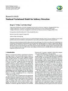
(a) (b) (c) (d) Fig. 5: PR curves and F-measure curves for different methods. (a) PR curves on MSRA5000 dataset. (b) PR curves on PASCAL1500 dataset. (c) F-measure curves on MSRA5000 dataset. (d) F-measure curves on PASCAL1500 dataset.
MSRA5000
PASCAL1500
TABLE I: Quantitative Ours RBD Precision(AT) .8105 .7824 Recall(AT) .7269 .6470 F-measure(AT) .7696 .7222 AUC .9192 .9127 MAE .0927 1106 Precision(AT) .6682 .6343 Recall(AT) .6488 .5724 F-measure(AT) .6231 .5749 AUC .8676 .8728 MAE .1420 .1539
Results For Different Methods. FPISA MSS HS PCA .7979 .6256 .6200 .5569 .4991 .6959 .6940 .5117 .6688 .6260 .6156 .5262 .8923 .9189 .8988 .9022 .1307 .1489 .1620 .1888 .6650 .5223 .4923 .4840 .3306 .6006 .6243 .4323 .4754 .5092 .4851 .4270 .8144 .8723 .8433 .8549 .2223 .1861 .1739 .2092
when q and j are in different regions, there exists at least one strong edge ( dcol (∗, ∗) ≥ 3σcol ) on their shortest path and wqj ≈ 0, ensuring that the saliency of j should not contribute to the saliency of q. σcol is the deviation for all dcol (∗, ∗) and computed in practice. Fig. 4 (c) and (d) show the comparisons based on our refinement methods and the upsampling proposed in [10] and our method performs better.
SF .7494 .2976 .5079 .8616 .1660 .6058 .1901 .3491 .8088 .1920
HC .4706 .5644 .4719 .7701 .2391 .3653 .4879 .3613 .7119 .2927
RC .4033 .5628 .4174 .8633 .2638 .3767 .5226 .3768 .8436 .2712
Fig. 6: Visual comparison of saliency maps of different methods, where from left to right, top to down are : input, HC [8], RC [8], SF [10], PCA [11], HS [27], MSS [23], FPISA [26], RBD [25], ours and ground-truth.
III. E XPERIMENT We evaluate and compare with other methods the performance of the proposed algorithm on two widely used datasets: MSRA5000 [20] and PASCAL1500 [26]. The MSRA5000 contains 5000 images with pixel-level ground-truths, while the PASCAL1500 which contains 1500 images with pixellevel ground-truths is more challenging for testing because they have more complicated patterns in both foreground and background. Then, we compare our results with eight state-ofthe art methods, including HC [8], RC [8], SF [10], PCA [11], FPISA [26], HS [27], MSS [23], RBD [25], among which are discussed and evaluated in the benchmark paper [7]. In the study, we use 4 standard criteria for quantitative evaluation, i.e., precision-recall (PR) curve [23], F-measure [27], Mean Absolute Error (MAE) [10], [25] and AUC score [11], [23]. For the PR curve, it is given in Fig. 5(a) and (b) by comparing the results with the ground-truth through varying thresholds within the range [0, 255]. And F-measure curve in Fig. 5(c) and (d) is drawn with different Fβ values calculated from the adaptive thresholded saliency map, where 2 )precision·recall 2 Fβ = (1+β β 2 ·precision+recall , and β = 0.3. The figures show that our approach achieves the better for these two measures. Specially, similar to [10], [26], in TABLE I we show the precision, recall and F-measure values for adaptive threshold (AT), which is defined as twice the mean saliency of the image. It still shows that the proposed method achieves the best on
these data. In addition, MAE is used to evaluate the averaged degree of the dissimilarity and comparability between the saliency image and the ground-truth at every pixel, and AUC score is calculated based on the true positive and false positive rates. It is shown in TABLE I that the proposed method presents the smallest MAE to denote our saliency maps are more close to the ground-truth at pixel level, and also offers satisfactory AUC scores compared with the others. Finally, Fig. 6 shows series of saliency maps of different methods. And it shows that our result has a great improvement over previous methods. W.r.t. the computational efficiency, the above average runtime for an input image is 1.67s in Matlab platform on a PC with Intel i5-4460 CPU and 8GB RAM. IV. C ONCLUSION In this letter, an effective bottom-up saliency detection method with the so-called spaces of background-based distribution (SBD) is presented. In order to describe the background distribution, some metric spaces of SBD are constructed, i.e., the elements are generated with eigendecomposition, plus the metric is designed carefully where the Mahalanobis distance is quoted to measure the saliency value for each patch. Further by enhancement in Bayesian perspective and refinement with geodesic distance, the whole salient detection is done. Finally,
5
the evaluational experiments exhibit the effectiveness of the proposed algorithm compared with the state-of-art methods. R EFERENCES [1] H. Ahn, B. Keum, D. Kim, and H. S. Lee, “Saliency based image segmentation,” in ICMT, 2011, pp. 5068–5071. [2] Z. Ren, S. Gao, L. T. Chia, and I. W. H. Tsang, “Region-based saliency detection and its application in object recognition,” IEEE Trans. Circuits and Syst. Video Technol., vol. 24, no. 5, pp. 769–779, 2014. [3] A. Li, X. She, and Q. Sun, “Scolor image quality assessment combining saliency and fsim,” in Fifth International Conference on Digital Image Processing., 2013, pp. 88780I–88780I. [4] R. Margolin, L. Zelnik-Manor, and A. Tal, “Saliency for image manipulation,” The Visual Computer, vol. 29, no. 5, pp. 381–392, 2013. [5] G. Zhang, Z. Yuan, N. Zheng, X. Sheng, and T. Liu, “Visual saliency based object tracking,” in ACCV, pp. 193–203. 2010. [6] A. Borji, M.-M. Cheng, H. Jiang, and J. Li, “Salient object detection: A survey,” arXiv preprint arXiv:1411.5878, 2014. [7] Ali Borji, Ming-Ming Cheng, Huaizu Jiang, and Jia Li, “Salient object detection: A benchmark,” IEEE Trans. Image Process., vol. 24, no. 12, pp. 5706–5722, 2015. [8] M.-M. Cheng, N. J. Mitra, X. Huang, P. H. Torr, and S. Hu, “Global contrast based salient region detection,” IEEE Trans. Patt. Anal. and Mach. Intell., vol. 37, no. 3, pp. 569–582, 2015. [9] Z. Liu, W. Zou, and O. Le Meur, “Saliency tree: A novel saliency detection framework,” IEEE Trans. Image Process., vol. 23, no. 5, pp. 1937–1952, 2014. [10] F. Perazzi, P. Kr¨ahenb¨uhl, Y. Pritch, and A. Hornung, “Saliency filters: Contrast based filtering for salient region detection,” in CVPR, 2012, pp. 733–740. [11] R. Margolin, A. Tal, and L. Zelnik-Manor, “What makes a patch distinct?,” in CVPR, 2013, pp. 1139–1146. [12] X. Li, H. Lu, L. Zhang, X. Ruan, and M. H. Yang, “Saliency detection via dense and sparse reconstruction,” in ICCV, 2013, pp. 2976–2983. [13] C. Yang, L. Zhang, H. Lu, X. Ruan, and M. H. Yang, “Saliency detection via graph-based manifold ranking,” in CVPR, 2013, pp. 3166–3173. [14] Y. Wei, Fang. Wen, W. Zhu, and J. Sun, “Geodesic saliency using background priors,” in ECCV, pp. 29–42. 2012. [15] S. Frintrop, T. Werner, and G. M. Garc´ıa, “Traditional saliency reloaded: A good old model in new shape,” in CVPR, 2015, pp. 82–90. [16] H. Jiang, J. Wang, Z. Yuan, Y. Wu, N. Zheng, and S. Li, “Salient object detection: A discriminative regional feature integration approach,” in CVPR, 2013, pp. 2083–2090. [17] J. Han, D. Zhang, X. Hu, L. Guo, J. Ren, and F. Wu, “Background prior based salient object detection via deep reconstruction residual,” IEEE Trans. Circuits and Systems for Video Technology, vol. 25, no. 8, pp. 1309–1321, 2014. [18] E. Rahtu, J. Kannala, M. Salo, and J. Heikkil¨a, “Segmenting salient objects from images and videos,” in ECCV, pp. 366–379. 2010. [19] S. Li, H. Lu, Z. Lin, X. Shen, and P. Brian, “Adaptive metric learning for saliency detection,” IEEE Trans. Image Process., vol. 24, no. 11, pp. 3321–3331, 2015. [20] T. Liu, Z. Yuan, J. Sun, J. Wang, N. Zheng, X. Tang, and H.-Y. Shum, “Learning to detect a salient object,” IEEE Trans. Patt. Anal. and Mach. Intell., vol. 33, no. 2, pp. 353–367, 2011. [21] J. Li, M. D. Levine, X. An, X. Xu, and H. He, “Visual saliency based on scale-space analysis in the frequency domain,” IEEE Trans. Patt. Anal. and Mach. Intell., vol. 35, no. 4, pp. 996–1010, 2013. [22] Y. Xie and L. Hu, “Visual saliency detection based on bayesian model,” in ICIP, 2011, pp. 645–648. [23] N. Tong, H. Lu, L. Zhang, and X. Ruan, “Saliency detection with multiscale superpixels,” IEEE Signal Processing Letters, vol. 21, no. 9, pp. 1035–1039, 2014. [24] Z. Li and J. Chen, “Superpixel segmentation using linear spectral clustering,” in CVPR, 2015, pp. 1356–1363. [25] W. Zhu, S. Liang, Y. Wei, and J. Sun, “Saliency optimization from robust background detection,” in CVPR, 2014, pp. 2814–2821. [26] K. Wang, L. Lin, J. Lu, C. Li, and K. Shi, “Pisa: Pixelwise image saliency by aggregating complementary appearance contrast measures with edge-preserving coherence,” IEEE Trans. Image Process., vol. 24, no. 10, pp. 3019–3033, 2015. [27] Q. Yan, L. Xu, J. Shi, and J. Jia, “Hierarchical saliency detection,” in CVPR, 2013, pp. 1155–1162.