Marine Resource Economics, Volume 23, pp. 273–293 Printed in the U.S.A. All rights reserved
0738-1360/00 $3.00 + .00 Copyright © 2008 MRE Foundation, Inc.
A Bioeconomic Analysis of a Wild Atlantic Salmon (Salmo salar) Recreational Fishery JON OLAF OLAUSSEN Trondheim Business School and Sintef Fisheries and Aquaculture ANDERS SKONHOFT Norwegian University of Science and Technology Abstract A biomass model of a wild salmon (Salmo salar) river recreational fishery is formulated, and the ways in which economic and biological conditions influence harvesting, stock size, profitability, and the benefit of the anglers are studied. The demand for recreational angling is met by fishing permits supplied by myopic profit-maximizing landowners. Both price-taking and monopolistic supply is studied. These schemes are contrasted with an overall river management regime. Gear regulations in the recreational fishery, but also the commercial fishery, are analysed under the various management scenarios, and the paper concludes with some policy implications. One novel result is that imposing gear restrictions in the recreational fishery may have the exact opposite stock effects of imposing restrictions on the marine harvest. Key words Salmon, recreational fishery, conflicting interests, stock dynamics. JEL Classification Codes Q26, Q22, Q21.
“River fisheries are a natural resource of a very limited character, and would be rapidly exhausted, if allowed to be used by every one without restraint” (John Stuart Mill 1848).
Introduction There has not been much good news concerning the abundance of wild salmon stocks in the North Atlantic during the last few decades. Stock development has been especially disappointing in the 1990s due to a combination of factors, such as sea temperature, diseases, and human activity, both in the spawning streams and through the strong growth of sea farming (NASCO 2004). Norwegian rivers are the most important spawning rivers for the East Atlantic stock, and about 30% of the remaining stock spawns here. The wild salmon are harvested by commercial and recreational fisheries. The marine harvest is mainly commercial, whereas the harvest in the spawning rivers is recreational. As the wild stock began to decrease during the 1980s, the Norwegian government imposed gear restrictions to limit the commercial Jon Olaf Olaussen is associate professor at Trondheim Business School, Sør-Trøndelag University College, NO-7004 Trondheim, Norway, and researcher at Sintef Fisheries and Aquaculture, NO-7065 Trondheim, Norway, email:
[email protected] Anders Skonhoft is a professor in the Department of Economics, Norwegian University of Science and Technology, NO-7491 Trondheim, Norway, email:
[email protected] Constructive comments from Lee G. Anderson, Claire Armstrong, and two anonymous reviewers are gratefully acknowledged. Jon Olaf Olaussen also thanks the Norwegian Research Council for funding.
273
274
Olaussen and Skonhoft
harvest. Drift net fishing was banned in 1989, and the fishing season of bend nets was restricted. At the same time, the fishing season in the spawning rivers was limited. However, despite all of these measures to rebuild the stock, the abundance of salmon seems to be only half the level experienced in the 1960s and 1970s. The same sad picture is observed other places (NASCO 2004). After drift net fishing was banned, catches by commercial fishermen and recreational anglers have been approximately equal (NOU 1999). In this article, however, we focus on the recreational fishery, as it is more important from an economic perspective. The value of the marine harvest is more or less directly related to the meat value, whereas recreational fishermen typically pay for the right to fish, and the high willingness to pay implies that the payment per kilo of fish caught is several times the meat value (NOU 1999). Altogether, there remain about 500 streams with spawning Atlantic salmon in Norway, and sport fishing is an important recreational activity. In addition, the indirect economic effects from the river fishery are of great importance to many local communities (Fiske and Aas 2001). The aim of this article is to analyse how biological and economic factors affect harvest, stock growth, the economic benefit, and the distribution of economic benefits among anglers and landowners in a representative Norwegian salmon river. A bioeconomic biomass model is formulated where the demand for fishing is given in number of days, whereas the quality of the river, approximated by average catch per fishing day, shifts demand up. On the supply side, there are a fixed number of landowners, treated as a single agent, managing the fishery under the assumption of profit maximization. Two different management regimes are studied; price-taking and monopolistic behaviour. Under both these schemes, it is assumed that the management is myopic. There may be various reasons leading to myopic management; most important is the presence of insecure property rights due to the marine harvest (see below). These management schemes are then contrasted with an overall river management solution. The model is illustrated by using ecological data from the river Imsa located on the southwestern coast of Norway (Rogaland County). There is a substantial literature on recreational fishing.1 The present model essentially builds on the sequential harvesting model of Charles and Reed (1985), but it is also related to Laukkanen (2001) who analyses the northern Baltic salmon fishery. We depart from Laukkanen’s paper as we study the recreational river fishery in more detail, while keeping the marine fishery in the background. In addition, and in contrast to Laukkanen (2001) and Charles and Reed (1985), the control variable in our analysis is fishing permits, not catch. Moreover, we differ from the traditional recreational fishing literature in that we explicitly consider the distribution of benefits between anglers and landowners (but see Anderson 1980b; Skonhoft and Logstein 2003). The effects of gear regulations in the commercial and the recreational fisheries are also analysed. The present model is closely related to Skonhoft and Logstein (2003), but they analysed monopolistic management in biological equilibrium only. However, various management schemes do not influence only harvest and stock level, but also the dynamics. One typical difference between small and medium/large salmon rivers seems to be that the yearly stock and catch statistics fluctuate much more from year to year in the small ones (Statistics Norway 2006). Since small rivers typically are managed more in accordance with a price-taking than a monopolistic management
1
The demand for sport fishing has been analysed and estimated in a wide range of papers, including Anderson (1980b, 1983, 1993); Layman, Boyce, and Criddle (1996); Green, Moss, and Spreen (1997); Provencher and Bishop (1997); and Schuhmann (1998). Studies of recreational versus commercial fisheries include McConnell and Sutinen (1979); Bishop and Samples (1980); Anderson (1980a); Rosenman (1991); Sutinen (1993); Cook and McGaw (1996); and Laukkanen (2001). Policy measures are analysed by Anderson (1993); Homans and Ruliffson (1999); and Woodward and Griffin (2003).
Atlantic Salmon Recreational Fishing
275
scheme (Fiske and Aas 2001), an unexplored question is if the different dynamic patterns may be an expected outcome due to different management regimes. Analysing fluctuations and dynamic patterns in a deterministic model means that we are interested in how steady state may be reached when facing an initial situation of overfishing or when certain factors (environmental or economic) have temporarily shocked the system out of equilibrium. Although the application is for an Atlantic salmon recreational fishery, the model yields general results with policy relevance to other recreational fisheries in, say, Scandinavia and North America. For example, while Norwegian Atlantic salmon fisheries are predominated by private ownership, the state is also a large landowner in some rivers. On the contrary, while national or state authorities provide most fishing permits in the USA, exceptions where riparian right holders possess exclusive rights to fish also exist (see Murphy and Stephenson 1999). Moreover, access and effort limitations, such as closed seasons and closed areas, are increasingly used in the USA in both fresh and saltwater recreational fisheries (Cox and Walters 2002, p. 117). The variety of management regimes in recreational fishing typically ranges from the type characterised by strong rights to public access of fishing opportunities in New Zealand as opposed to the strong protection of private property rights in all freshwater fisheries in Scotland. However, in the recreational fishing literature, management regimes are typically adopted from the commercial fishing literature focusing on open-access and sole-owner schemes only. The rest of the article is structured as follows. In the next section, we formulate the biological model and introduce harvesting. Then, the cost and benefit functions are formulated, and today’s practice of myopic management is analysed based on price-taking and monopolistic landowners, respectively. Next, we study the overall river management solution. Finally, numerical analysis and results are presented before the article concludes with some policy recommendations.
Population Dynamics and Biological Equilibrium Building on Charles and Reed (1985), we consider a salmon sub-population whose size in biomass (or number of fish) at the beginning of the fishing season in year t is Xt. Both a marine and a river fishery influence the population during the spawning migration from its offshore environment to the coast and its parent river (‘the home river’) where reproduction takes place. A fixed fraction, σ, of the adult stock is assumed to leave the offshore habitat each year (Mills 1989) (see figure 1). The marine fishery first influences the stock, because marine harvest takes place in fjords and inlets before the salmon reaches its spawning river. For a marine harvest rate 0 ≤ h ≤ 1, hσXt fish are removed from the population. The escapement to the home river is accordingly (1 – h)σXt. The river fishery exploits this spawning population along the upstream migration. When the river harvesting fraction is 0 ≤ yt ≤ 1, the river escapement is (1 – yt)(1 – h)σXt. This spawning stock yields a subsequent recruitment R[(1 – yt)(1 – h)σXt] to next year’s stock. It is assumed that the stockrecruitment relationship, R(.), is purely compensating so that R′ > 0 (more details below).2 The fraction of the recruits that survive is s2. When a further (quite small) 2
As the juveniles usually spend several years in the river before they start their downstream migration and eventually join the offshore stock, the model represents a simplification of reality. This is due to the biomass approach, which could be made more realistic by a more detailed ecological model, including the age structure of the stock. Strictly speaking, therefore, each step in the time index, t, represents an average salmon generation life time (which varies between three and five years in different rivers) rather than one year. Laukkanen (2001) applies the same biomass approach.
276
Olaussen and Skonhoft
Figure 1. Harvest and Reproduction Scheme
proportion, s1, of the spawners survive to be part of the stock the next year, and a proportion, s 0, of the nonspawners staying offshore similarly survives (see Mills 1989 and 2000 for details), the population dynamics follows as: X t+1 = s 2 R((1 – y t )(1 – h)σX t) + s 1 (1 – y t )(1 – h)σX t + s 0(1 – σ)X t .
(1)
Generally, when a single fish population is harvested sequentially by separate fisheries, as here, there will be conflicts between the different groups of harvesters because the size of h will influence the size of yt, but also vice versa through next year’s fisheries. Hence, there will be reciprocal externalities present (see McKelvey 1997). The present analysis is, however, restricted to studying the exploitation of the river fishery while taking the marine salmon fishery as given. The main reason for doing so is that we want to analyse the sport fishery thoroughly, as this is by far the most important part of the salmon fishery (see above). However, we do examine how the marine harvest affects the harvest and benefits of the recreational fishery by analysing shifts in the (exogenous) marine harvesting rate. These shifts may be interpreted as changing restrictions imposed on the marine fishery; e.g., changes in season length, size and type of nets, and so forth. Therefore, given the marine harvest rate, we focus on the river offtake Yt = yt(1 – h)σX t. As discussed further in the next section, the market for the salmon recreational fishery is related to the number of daily fishing permits, Dt, sold throughout the season (June–August). Accordingly, the number of fishing permits, or the number of fishing days spent in the river, represents the effort in the river fishery. We assume a harvesting function of the Schaefer type: Y t = qD t(1 – h)σX t,
(2)
where q is the productivity (‘catchability’) coefficient related to the type of fishing
Atlantic Salmon Recreational Fishing
277
equipment (fly fishing, fishing lure, spinning bait, and so forth)3 and with (1 – h)σXt as the stock available for sport fishing (see above). When combining the catch function (2) with the river offtake (Yt = yt(1 – h)σXt), we find the harvesting fraction in the river simply as yt = qDt. Inserted into the population dynamic equation (1), the stock growth yields Xt+1 = s2R[(1 – qDt)(1 – h)σXt] + s1 (1 – qDt)(1 – h)σXt + s0(1 – σ)Xt. This may also be written as X t+1 = F(Xt, D t), where ∂F/∂D t = FD < 0 holds. In addition, we find that 0 < FX < 1 under the present assumption of a pure compensatory stock-recruitment function (R′ > 0). When Xt = Xt+1 = X and Dt = D, the stock-effort equilibrium is written as: X = F(X,D).
(3)
Implicitly, this biological equilibrium condition defines the equilibrium stock as a function of the number of fishing days. Differentiation yields (1 – FX)dX = FDdD. Hence, more effort means a smaller stock. Therefore, the stock-effort equilibrium condition is negatively sloped in the X – D diagram, and, where D = 0, it produces the highest possible stock level, whereas X = 0 gives the highest number of fishing days incompatible with an equilibrium fishery (see figure 2). We find that the biological equilibrium shifts inwards if the marine harvest rate, h, shifts up. This is in line with intuition, since in order to keep a given stock, X, a higher marine harvest rate must be accompanied by a reduced effort in the river. A higher catchability coefficient, q, shifts the biological equilibrium condition inwards for the same reason. That is, in order to keep a given stock size, increased catch efficiency must be accompanied by reduced effort.
Demand and Cost Functions We now introduce a market for sport fishing in our representative spawning river. On the demand side, there is a large number of potential recreational anglers, while there is a fixed number of landowners along the river who are given the right (by the State) to sell fishing permits (NOU 1999). These landowners are treated as a single agent, as they in most instances join forces and establish a river owner association. The competition from landowners in other rivers may vary. Crucial factors are the distance, which may vary between some few kilometres to over hundred kilometres, transportation costs, and various river-specific attributes. In most instances, the market situation is probably something between price-taking and monopoly behaviour (Skonhoft and Logstein 2003). However, we study both these market forms as stylized extremes. The price-taking case typically corresponds to the situation in fjords holding many salmon rivers competing for the same anglers, while the monopolistic case, on the other hand, corresponds to fjords with just one dominating river.4 As mentioned, the market for salmon recreational fishing is related to the number of daily fishing permits sold (see McConnell and Sutinen 1989; Anderson 1983, 1993; and Lee 1996). Fishing permits may be for one day, one week, or a whole sea3
The assumption of a fixed catchability coefficient has been subject to criticism. Arrenguin-Sanchez (1996) provides a review. A related issue is the linearity assumption in number of fishing days in the catch function, cf. the above Schaefer function. Among others, Anderson (1993), Homans and Ruliffson (1999), and Woodward and Griffin (2003) formulate recreational fishing models where this assumption is relaxed. However, the linearity assumption yields a simple, tractable relationship between the harvesting fraction and effort (main text below). 4 An example of this first case is the fjord Nordfjord on the western coast with the rivers Strynelva, Loenelva, Oldenelva, Gloppenelva, Gjengedalsvassdraget, Straumeelva, Hopeelva, and Eidselva. The fjord Altafjord with the river Alta in the far northern part of Norway is an example of the other case.
278
Olaussen and Skonhoft
Figure 2. Economic and Biological Equilibria Notes: X is stock size in number of salmon, D is fishing effort in number of fishing days. Superscript P denotes myopic price taking landowners, superscript M denotes myopic monopolistic landowners, and superscript * denotes overall management.
son. However, we collapse all these possibilities into one-day permits only, so that the market demand is directly expressed in number of day permits, Dt, and is in a standard manner decreasing in permit price. The sport fishermen’s notion of the river quality is assumed to influence demand as well. In line with McConnell and Sutinen (1979), it is expressed as the average catch per day, and for a given number of fishing days, a higher catch per day shifts the demand function upwards.5 The inverse market demand for fishing licenses is given as: Pt = P ( Dt , v t ),
(4)
where Pt is the fishing permit price per day, and vt is the demand-induced catch per day.6 In the present exposition, the demand is the residual after potential travel costs have been subtracted. We have vt = θQt and, where catch per day (as a quality mea5
It is tacitly assumed that the anglers are homogeneous in all relevant aspects of the model (see Anderson 1993 that allows for heterogeneous anglers). However, as pointed out by one of the reviewers, relaxing this assumption may produce different welfare results, as different anglers may react differently to both price and quality changes. 6 The implicit assumption underlying this demand function is that the recreational participants know the current year’s stock size and how it translates into catch per day. A lagged model where the expected catch is based on previous years catch rates, is an alternative formulation. Such a demand function will complicate the dynamics of the model (we will then at least have a second-order non-linear difference equation, see below). However, under quite mild conditions, it will not affect the equilibrium (see Gandolfo 1996 for a theoretical exposition).
Atlantic Salmon Recreational Fishing
279
sure) from the catch function (2) is seen to be proportional to the river escapement, Qt = Y t / Dt = q(1 – h)σXt . The parameter θ > 0 indicates how catch per day translates into demand. Obviously, the quality effect will vary between rivers, and it may change over time. For these and others reasons, it is difficult to assess the strength of the quality effect, but on the whole, we may interpret θ as a parameter measuring how important the catch is compared to other factors influencing demand.7 Hence, in addition to PD < 0, we have Pv > 0. When inserting catch per day into the inverse demand condition (4), the current profit of the landowner is:
π t = P ( Dt , v t ) Dt − C ( Dt ),
(5)
where C(Dt) is the cost function, covering fixed as well as variable costs with C′(Dt) > 0 and C″(D t) ≥ 0. Fixed costs include various types of costs associated with preparing the fishery (constructing tracks, fishing huts, and so forth), whereas variable costs include the costs of organizing the fishing permit sales together with enforcement. The planning horizon of the landowner is important. As there are many rivers and landowners, various planning horizons may be present. We will compare longterm planning in the case of an overall river manager with myopic landowners. This is not to say that all landowners are myopic. However, to cultivate this difference, we consider a myopic landowner only, meaning that the landowner (i.e., the landowner association), supplies fishing permits in the given river based on current economic and biological conditions. There may be various reasons leading to myopic management; most important is the presence of insecure property rights due to the marine harvest. Other factors, such as ecological and environmental uncertainties (which are not taken into account in the present analysis), are also of importance.8 The traditional view that even a small number of spawners is sufficient to fully recruit a salmon river may play a role as well. Such myopic behaviour seems to be in accordance with the stylized facts management situation in the Norwegian salmon river fishery (Skonhoft and Logstein 2003) and implies that exploitation takes place under a kind of unregulated common property rights structure (see Bromley 1991 for an excellent treatment). This is the same resource management scheme studied in numerous papers (e.g., Brander and Taylor 1998). Myopic exploitation is studied both under the price-taking and monopolistic landowner assumption and is, as mentioned, compared with the long-term planning of an overall river manager.9
7
Using this simple demand function obviously means that many factors (income, average size of the fish caught, accommodations, congestion, and so forth) are neglected. However, our formulation seems to capture two of the most important demand elements. In a Norwegian survey, 92% of the sport fishermen reported that the quality of the river with respect to average catch per day was important. In addition, 72% reported that the price of fishing permits was important (Fiske and Aas 2001). 8 In a Norwegian survey, 73% of the river owners reported that stock uncertainty was a very important reason for not investing in salmon fishing tourism (Birkelund, Lein, and Aas 2000). 9 Note that this is not the same as the classical open-access solution. In the classical open-access situation, more fishermen enter the fishery until the rent is dissipated. If the productivity of the fishermen is equal, there will be no rent at all, while an intra marginal rent is present when productivity differs. Under myopic conditions, the landowner (i.e., the landowner association) simply maximises current profit while taking the stock as given; i.e., the stock effect is ignored. However, the profit may be zero under this assumption as well, and this certainly happens under the combination of price taking behaviour and constant marginal costs (see numerical section).
280
Olaussen and Skonhoft
Price-Taking Landowner First, we look at the situation where fishing permits are supplied under price-taking behaviour, for example because there are many rivers located in the fjord. When also supplying fishing permits under myopic conditions, the landowner maximizes the current profit [equation (5)] with respect to the number of fishing permits, while taking the price as well as the stock as given. The first-order condition is: P ( Dt , v t ) – C ′( Dt ) = 0.
(6)
This condition defines the function D t = DP(X t) (superscript P is for price-taking behaviour). When inserted into the population dynamic equation (1), or X t+1 = F(X t,Dt), we obtain Xt+1 = F[Xt, D P(Xt)]. This is a first-order non-linear difference equation that, in principle, may exhibit all types of dynamics (see the classical May 1976). Therefore, the present myopic management scheme does not automatically secure any long-term equilibrium or steady state. However, it is a strong demandside stabilizing effect present as demand responds to the stock size through the quality factor. On the other hand, parameters in the stock-recruitment and harvesting functions may work in a destabilizing manner (more on this below). Supposing that a steady state exists, the first-order condition (6) represents the economic equilibrium condition P(D, v) – C′(D) = 0, and where differentiation yields [PD – C″]dD = –θq(1 – h)σ PvdX. As the left-hand side is negative due to the second-order condition for maximum, we find this equilibrium condition, if existing, to be positively sloped in the X – D plane. In line with intuition, a higher stock size is associated with more fishing days in economic equilibrium (figure 2). Therefore, the economic equilibrium condition simply tells us that at a given price a higher fish stock means that more fishing permits are sold. Moreover, this means that the intersection with the negatively sloped biological equilibrium condition (3) represents the (unique) bioeconomic equilibrium XP, DP under the present myopic price-taking management scheme. The total river surplus comprises the landowner profit and the angler surplus (consumer surplus). At a given point of time, as well as in the steady state, the angler surplus is given by the area under the inverse demand function for a given stock size (or the given demand-induced catch per day). A higher stock size for the same market price yields a higher angler surplus as the inverse demand function shifts up. However, because the stock is not controlled by the landowners or the anglers, XP is considered to be an externality determining the value of the angler surplus, as well as the profit (Anderson 1983). This will also be the case outside the bioeconomic equilibrium. Throughout the reminder of the article, two important comparative static, as well as dynamic, effects are analysed; shifts in the marine harvest rate, h, and the catchability coefficient, q. As mentioned above, a shift in the marine harvest rate may be interpreted as changes in the restrictions imposed on the marine fishery by the State. Likewise, a shift in the catchability coefficient can be related to new gear regulations in the river fishery and where, say, a reduction in q may be due to banning of different bait types.10 It can easily be shown that a higher marine harvest rate, h, shifts the economic equilibrium condition outwards, meaning that lower effort is compatible with the same fish stock. As a higher marine harvest rate shifts the biological equilibrium in10
Fiske and Aas (2001) present an overview of the efficiency of different angling methods in recreational salmon fishing.
Atlantic Salmon Recreational Fishing
281
wards (see the Population Dynamics and Biological Equilibrium section above), we find that the number of fishing permits decreases, whereas the equilibrium stock effect is generally ambiguous. If the demand response is weak, the stock will decrease with a higher marine harvest rate, h. On the other hand, if the demand response is strong; that is, the quality parameter θ has a high value, we may find that the equilibrium stock increases (more on this in the numerical example below). An increased catchability coefficient q (e.g., relaxed gear restrictions) shifts the economic equilibrium condition inwards. Again, this follows intuition, since a higher catchability increases demand through increased quality of the fishing experience (increased catch per fishing day). Hence, for a given stock size, X, increased catchability is accompanied by greater effort. As the biological equilibrium condition also shifts inwards with a higher q (see Population Dynamics and Biological Equilibrium section above), we find that the equilibrium stock (if an equilibrium exists) decreases, while the effect on the number of fishing days is ambiguous. It can be shown that the sign of this effort effect (number of fishing days) depends on the quality demand response through θ. If the demand response is strong; that is, the quality parameter θ has a high value, the possibility of a positive effort effect increases. More generally, the shift in economic equilibrium pulls in the direction of a higher effort, while the shift in biological equilibrium pulls in the other direction. In any case, we find that relaxing the gear restrictions in the recreational fishery always decreases the salmon stock, while relaxing the restrictions in the marine fishery, and thereby increasing the marine harvest rate, h, may in fact increase the stock through reduced recreational demand (see the numerical section below). The total surplus and the surplus distribution between the landowner and the anglers will be influenced both by h and q. However, the outcomes are quite complex because of the quality effect in the demand function. If a higher marine harvest fraction is accompanied by a smaller stock, together with a lower number of fishing permits, angler surplus decreases. This may also be true for landowner profit (but not with constant marginal cost, see below). However, which components are reduced most depends on circumstances. The picture is even more complex if a higher h is accompanied by more salmon (more on this in the numerical analysis).
Monopolistic Landowner We now study the other stylised management scheme where the landowner (i.e., the landowner association) acts as a monopolistic supplier of fishing permits. As mentioned above, there may be various reasons leading to monopolistic myopic management. The actual river is then typically located far away from other rivers, so it is possible to exercise market power. At the same time, insecure property rights due to the marine harvest activity and the traditional view that only a few spawners are required to fully recruit a salmon river, both pull in the direction of myopic behaviour and neglecting the effect on the future stock. Under monopolistic and myopic behaviour, maximizing equation (5) with respect to D t yields the first-order condition:
P ( Dt , v t ) + PD ( Dt , v t ) D – C ′( Dt ) = 0.
(7)
Equation (7) defines the function Dt = D M(X t) (superscript M is for monopolistic behaviour). Inserted into the population growth function (1), or Xt+1 = F(Xt, Dt), we again obtain a first-order non-linear difference equation. It is difficult to say how this difference equation behaves compared to the price-taker situation. However, as
282
Olaussen and Skonhoft
monopolistic management is more conducive to stock conservation (see below), one may suspect that fluctuations, if any, will be more modest than in the price-taking case. As explained above, such fluctuations may be due to a temporal situation of overfishing. Supposing that a steady state exists, the first-order condition (7) yields the monopolistic economic equilibrium condition P(D, v) + P D(D, v)D – C′(D) = 0. Differentiation gives [2PD + DPDD – C″]dD = –θq(1 – h)σ[Pv + DP Dv]dX, where the term in the bracket on the left-hand side again is negative due to the second-order condition. Under the reasonable assumption that the quality effect dominates the potentially negative cross effect in the demand function, so that [Pv + DP Dv] > 0, we find that the economic equilibrium condition again is positively sloped in the X–D diagram. However, it is less positively sloped than the economic equilibrium condition under price-taking behaviour. The intuition is straightforward as a higher fish stock increases the demand for fishing permits, as in the case of the myopic pricetaking landowner. Since increasing demand is accompanied by a higher permit price in the monopolistic case, the permit sale increases less than under price-taking behaviour. Notice also that the intercepts of the first-order conditions (6) and (7) with the X-axis are the same (again, see figure 2). For these reasons, as expected, the bioeconomic equilibrium stock is higher and the number of supplied permits is lower than under price-taking behaviour; that is, XM > XP and DM < DP. Hence, in accordance with most natural resource economic models, the monopolistic exploitation regime is more resource conserving than the price-taking regime (e.g., Hanley, Shogren, and White 1997). While the monopolistic scheme yields more fish and less effort in bioeconomic equilibrium than the price-taking scheme, the total surplus will not necessarily be higher. The reason is that the quality effect in the demand function works like an externality (see above). Hence, higher profit may be dominated by a reduced angler surplus when moving from the myopic monopolistic scheme to the myopic pricetaking scheme (cf. the numerical results). Depending on how the demand curve shifts, it is also possible, at least in theory, that angler surplus can increase when moving to the monopolistic scheme.
The Overall River Management Solution The above two myopic management regimes are now contrasted with the overall river management solution (hereafter referred to as overall management), where the goal of the manager is to maximize the present value overall economic benefit, comprising landowner profit and angler surplus (consumer surplus), while taking the population dynamics into account. Hence, the goal of the overall manager is to maximize: ∞
⎡ Dt ⎤ ρ t ⎢ P ( ξ t , v t )dξ t − C ( Dt )⎥, ⎢⎣ 0 ⎥⎦
∑ ∫ t=0
subject to the population dynamics Xt+1 = F(Xt, D t). ρ = 1/(1+δ) is the discount factor, with δ > 0 as the (yearly) discount rate. The current value Hamiltonian of this problem reads: Dt
H ( X t , Dt , λ t + 1 ) =
∫ P(ξ , v )dξ t
0
t
t
− C ( Dt ) + ρλ t +1 [ F ( X t , Dt ) − X t ],
Atlantic Salmon Recreational Fishing
283
where λt > 0 is the resource shadow price (see Conrad and Clark 1995). The firstorder conditions yield: ∂H / ∂Dt = 0 → P ( Dt , v t ) − C ′( Dt ) + ρλ t +1FD ( X t , Dt ) = 0
(8)
ρλ t +1 − λ t = −∂H / ∂X t → ρλ t +1 − λ t
(9)
and
= − Pv ( Dt , v t )θqσ (1 − h ) Dt − ρλ t +1 [ FX ( X t , Dt ) − 1]
when assuming an interior solution (a positive supply of fishing permits at the steady state). The interpretation of control condition (8) is that fishing permits should be supplied up to the point where the licence price is equal to the marginal cost of the suppliers plus the cost of reduced stock growth, evaluated at the shadow price. Equation (9) is the portfolio condition governing the change of the resource price. Basically, it states that the biomass should be maintained so that the change in the net natural growth is equal to the (shadow) price change, adjusted for the discount factor. As the Hamiltonian is not linear in the control, we typically find that the dynamics will not be of the Most Rapid Approach Path (MRAP) (see the numerical analysis). Suppose that a steady state exists and is reachable from X0. Evaluating equation (8) at the steady state implies λ = –[P(D, vt) – C′(D)]/ρFD(X,D). Substituting equation (8) into equation (9), also in the steady state, and rearranging, we obtain the discrete time golden rule condition:
FX ( X , D ) −
[ Pv ( D, θQ )θqσ (1 −
h ) D]
P ( D, θQ ) − C ′( D )
FD ( X , D ) = 1 + δ,
(10)
which states that the internal rate of return of the resource should be equal to the external rate of return (1 + δ). The golden rule condition, together with the biological equilibrium condition (3), yields the overall management steady state X* and D*. This steady solution may be compared to the steady states (if existing) under myopic management. It is straightforward to demonstrate that the control condition (8) in economic equilibrium will have the same intercept with the X axis as in the price taking and monopolistic regimes because the shadow price of the stock is zero whenever there is no permit sale.11 Furthermore, it is seen directly that it will be located further outward than the price-taking equation (6) in equilibrium, because FD′ < 0 and λ > 0 (again, see figure 2). Therefore, we can conclude that the steadystate stock level will be higher and the number of fishing permits will be lower than under the myopic price-taking scheme; that is, X* > XP and D* < D P. Consequently, the fishing permit price following myopic price-taking management will always be below the overall management solution. Comparing with the monopolistic myopic solution (7) indicates that the overall management solution, depending on the difference (P DD – ρλF D ), will be located between the price-taking solution and the monopolistic solution if |PDD| > |ρλFD| and further outwards than the myopic monopolistic solution if |PDD| < |ρλFD|. The intuition is clear as a high discount factor; i.e., a low discount rate and a high shadow price of the stock both pull in the direc11 When evaluating equation (9) at steady state, we find λ(1 + ρF X) = Pv θqσ(1 – h)D after a small rearrangement. Hence, no permit sale and D = 0 is accompanied by λ = 0.
284
Olaussen and Skonhoft
tion of the overall management being more stock conserving than the myopic monopolistic regime. On the other hand, a low discount factor or a low shadow price of the stock pulls the overall management in the direction of the outcome of the myopic price taking management scheme. According to the discussion above, it is not possible to infer anything definite about the distribution of benefits between the anglers and landowners. The total current surplus in the myopic equilibria may be above that of the overall management equilibrium solution due to discounting.12 It can be shown that a higher periodic discount rate will increase the slope of the control condition (8) in equilibrium. Consequently, as discussed above, the steady state of the overall management solution approaches the price-taking myopic management solution. In the limiting case of δ = ∞, we find that the overall management solution coincides with the equilibrium price-taker myopic management situation. The steady-state total surplus and the distribution of the surplus are then equal in these regimes. On the other hand, when δ = 0, the steady state of the overall management solution coincides with the problem of total current surplus maximization in biological equilibrium.13 In this case, the total current surplus is obviously higher than under the myopic price-taking scheme. However, for intermediate values of the discount rate, the total current surplus may be higher in the price taking case due to discounting. This may also be so when comparing the overall management with the myopic monopolistic scheme.
Numerical Analysis and Results14 Data and Specific Functional Forms The above analysis will now be illustrated numerically with data from the river Imsa. This is a typically small, but productive, salmon river located on the southwestern coast of Norway (for details, see Hansen, Jonsson, and Jonsson 1996). We start by specifying the functional forms. The stock-recruitment function is given as the Cushing curve version of the Shepherd function (Shepherd 1982; King 1995):
R = R[(1 − qDt )(1 − h )σX t ] = r
(1 − qDt )(1 − h )σX t ⎡ (1 − qDt )(1 − h )σX t ⎤γ 1+⎢ ⎥ K ⎣ ⎦
,
(11)
where (1 – qDt)(1 – h)σXt is the spawning biomass (see Population Dynamics and Biological Equilibrium section above), r > 0 is the intrinsic growth rate interpreted as the maximum number of recruits per spawning salmon, and K > 0 is the stock level for which density-dependent mortality equals density-independent mortality. The compensation parameter, γ > 0, indicates to what extent density independent effects compensate for changes in stock size. The parameter values are estimated by
12 However, the present-value total surplus is obviously higher under the overall management than the present-value total surplus of the myopic solutions for the same time period and discount rate. 13 These results are the same as we find in the standard Clark harvesting model (see Munro and Scott 1985), except that the infinite discount rate yields the so-called open-access solution, while here it applies to the slightly different regime of myopic price taking exploitation (cf. also footnote 8). 14 The dynamic optimization was performed with the Solver tool bundled with Microsoft Excel. The code is made available under Numerical analysis fisheries management – Salmon management at www.svt.ntnu.no/iso/Anders.Skonhoft/default.htm
285
Atlantic Salmon Recreational Fishing Table 1 Baseline Parameter Values Parameter
Description
r
Maximum recruitment per spawning salmon
K
Stock level where density-dependent mortality dominates density-independent factors Degree to which extent density-independent effects compensate for stock changes Fraction of non-spawners Survival rate non-spawners Share of salmon spawning twice Survival rate, downstream smolt migration Reservation price when catch per day is 1 Price effect demand Marginal cost fishing permit sale Fixed cost fishing permit sale Catchability coefficient Marine harvest rate Period discount rate Quality response in demand
γ σ s0 s1 s2 α β c c0 q h δ θ
Value 124 (smolts per spawning salmon) 5.3 (number of spawning salmon) 0.77 0.85 0.5 0.25 0.4 400 (NOK/salmon) 1 (NOK/day2) 50 (NOK/day) 0 0.0025 (1/day) 0.4 0.07 1
Hansen, Jonsson, and Jonsson (1996) for Imsa and are reported in the table 1 (see also Appendix). Here, it can be seen that we have γ < 1 and the density-dependent effect is weak. Consequently, as already indicated, the stock-recruitment function (11) is increasing for all levels of the spawning population, R′ > 0. The inverse demand function is specified as linear. In addition, it is assumed that the quality of the river, approximated by demand induced catch per day, Vt = θq(1 – h)σXt, shifts the demand uniformly up: Pt = αv t – βDt .
(12)
Accordingly, the choke price, α, gives the maximum willingness to pay when the quality-translated catch is one fish per day, whereas β reflects the price response in a standard manner. The cost function is linear as well: C t = c0 + cDt ,
(13)
so that c 0 is the fixed cost, while c is the constant marginal cost of providing a fishing permit (see Demand and Cost Functions). Based on the above demand and cost functions, we find that the first-order condition under the myopic price taking and monopolistic schemes are avt – βDt = c and avt – 2βDt = c, respectively. It is therefore a linear, increasing relationship between stock size and the number of fishing days, and the slope of the economic equilibrium condition under price taking will be two times higher than that of the monopolistic case (cf. also figure 2). The economic baseline parameter values are found in table 1 (see Appendix).
286
Olaussen and Skonhoft
Steady States First, we look at the steady states. For the baseline parameter values, the steady state will be approached smoothly under all three management schemes. It can be seen in table 2 that the monopolistic myopic regime is somewhat more stock conserving than the overall management regime. As demonstrated above, the reason for this is that in order to increase profit, the monopolist reduces demand more than does the overall manager, who accounts for the future stock value. When the landowners face competition and act as price takers, the stock is substantially lower. On the contrary, and consistent with this, permit sales are higher and the license price is lower. Because of the constant marginal cost assumption, the price under the price-taking scheme just equalizes this value. In addition, under the baseline parameter values, it can be seen that the total surplus (angler and landowner surpluses) in the overall management and monopolistic cases are equal. This happens by accident, but as noted above it is possible that the steady-state total surplus in the myopic monopolistic case (as well as under price taking) can exceed the overall management surplus due to discounting (see The Overall River Management Solution). The total surplus in the myopic monopolistic case is above that of the myopic price-taking case. As explained in the Monopolistic Landowner section, the reason for this is the quality shift in the market demand function. However, the anglers are substantially better off under the myopic pricetaking scheme irrespective of the fact that the quality of the fishing experience,
Table 2 Steady State Results Parameter Values
Myopic Price Taker
Myopic Monopolist
Overall Management
X
Baseline values Catchability ↑
562 469
692 623
662 628
D
Baseline values Catchability ↑
237 237
152 166
173 163
P
Baseline values Catchability ↑
50 50
202 216
165 221
v
Baseline values Catchability ↑
0.72 0.72
0.88 1.06
0.85 1.02
LS
Baseline values Catchability ↑
0 0
23 27
20 28
AS
Baseline values Catchability ↑
28 28
12 14
15 13
TS
Baseline values Catchability ↑
28 28
35 41
35 41
Notes: Stock size, X (number of salmon); number of fishing days, D; permit price, P (NOK per day); v demand induced catch per day; landowner surplus LS (1,000 NOK); angler surplus AS (1,000 NOK); and total surplus TS (1,000 NOK). Catchability ↑; the catchability coefficient, q, increases by 20%. Notice that v corresponds to catch per day since θ=1 (table 1).
287
Atlantic Salmon Recreational Fishing
measured as catch per day, is lowest here. Thus, the low fishing license price more than compensates for the low quality. Note that the angler surplus is also higher under the price-taking regime than under overall management. Table 2 reports the results when the catchability coefficient increases by 20% due to relaxed gear restrictions. Stock abundance becomes substantially lower under the pricetaking scheme while stock effects are more modest in the monopolistic case and overall management case due to the increased fishing permit price. The catchability shift materializes into small changes in angler surplus, while landowner surplus increases most under overall management. Moreover, since the total surplus increases with more efficient fishing equipment, the opposite occurs when gear restrictions are imposed. Table 3 demonstrates how changes in the marine harvest rate, h, affect the steady-state river fishery, where h = 0.4 is the baseline value (see also table 2). A higher marine harvest rate through relaxed harvesting restrictions has an ambiguous stock effect under both myopic schemes, whereas the stock decreases under overall management. If the quality demand effect is strong, we obtain the somewhat para-
Table 3 Steady-state Results, Different Marine Harvest Rates Marine Harvest Rate, h 0.0
0.2
0.4
0.6
0.8
512 298 50 0.87 0 44 44
562 237 50 0.72 0 28 28
573 145 50 0.49 0 10 10
482 32 50 0.21 0 1 1
696 212 261 1.18 45 22 67
692 152 202 0.88 23 12 35
638 83 134 0.54 7 3 10
495 17 67 0.21 0 0 0
715 202 284 1.22 47 20 67
662 173 165 0.85 20 15 35
604 116 89 0.51 5 7 12
486 29 54 0.21 1 0 1
Myopic Price-taking Management XP DP PP vP LSP AS P TSP
453 335 50 0.96 0 56 56
Myopic Monopolistic Management XM DM PM vM LSM AS M TSM
671 260 310 1.43 68 34 102
Overall Management X* D* P* v* LS* AS * TS*
765 219 431 1.63 83 24 107
Notes: Stock size, X (number of salmon); number of fishing days, D; permit price, P (NOK per day); v demand induced catch per day; landowner surplus LS (1,000 NOK); angler surplus AS (1,000 NOK); and total surplus TS (1,000 NOK). Notice that v corresponds to catch per day since θ=1 (table 1).
288
Olaussen and Skonhoft
doxical result that a higher marine harvesting pressure goes hand in hand with more fish (see Price-Taking Landowner). Note that this is the exact opposite stock effect of that obtained by relaxing the gear restrictions in the recreational fishery under the myopic schemes (see discussion above). Under overall management, on the other hand, a higher h translates consistently into a smaller stock because the stock shadow price, from a river management point of view, depends on the fish biomass entering the river. Hence, when the marine harvest rate increases, the shadow price decreases. A higher h generally reduces the surplus.
Dynamics As mentioned in the introduction, one of the questions we want to reveal is whether type of management regime can explain any dynamic differences among different rivers; e.g., if small rivers exhibit more stock fluctuations because they are more likely to be managed in line with a price-taking scheme. For the given specific functional forms, the first-order myopic profit maximum conditions yield linear relationships between the number of fishing days and the stock. We have Dt = D P (Xt) = (1/β)[αvt – c] in the price-taking case and Dt = DM (Xt) = (1/2β)[αvt – c] in the monopolistic case. Therefore, these equations, combined with the population growth function (1), or X t+1 = F(Xt, Dt) and the stock-recruitment function (11), yield the first-order non-linear difference stock equations under the myopic schemes to be studied here. Figures 3a and b demonstrate the dynamics for the baseline parameterization of these myopic schemes, while figure 3c shows the overall management solution. The initial stock size is assumed to be quite modest (X 0 = 50), so these transitional growth paths demonstrate recovery from a previous situation involving serious overfishing, or possible deceases.15 The steady states are reached rapidly, with negligible overshooting, and the dynamics are quite similar under all three management scenarios. The same dynamic pattern is found when starting out with other initial values; e.g., with an initial stock that is very high. Hence, the dynamics is of the ergodic type, leading to the unique steady states. Based on the examination of different initial values, the overall management solution does not seem to be substantially different from the MRAP (see The Overall River Management Solution). As mentioned, the basic stabilizing factor when the stock is low is the quality factor in demand; that is, a low stock is accompanied by a modest demand and the stock rebuilds smoothly. In the same manner, the quality factor is also stabilizing when the stock is high, as a high stock is accompanied by a high demand that ultimately drives the stock down.16 Although the steady states under myopic management seem to be quite stable given the baseline parameter values, other ecological and economic conditions may produce instability. We find that relaxing the gear restrictions and thereby increasing the recreational fishery catchability coefficient, q, may induce all types of dynamics. For example, the dynamics will exhibit a two-point cycle pattern (see Conrad and Clark 1995) if q increases by 35% (see figure 4a). Furthermore, if q increases by
15
Outbreaks of Gyrodactylus salaris, Furunculosis, or sea lice infections are examples of such incidences (NOU 1999). 16 One interesting expansion of the model would be to include congestion demand effects. The resulting dynamic outcome is potentially ambiguous. On the one hand, the demand effect of a stock change will be reduced, possibly leading to larger stock fluctuations. On the other hand, ceteris paribus, the possibility of demand driven stock changes will occur is reduced since demand is more stable with congestion effects present.
Atlantic Salmon Recreational Fishing
289
Figure 3. Dynamic Paths Notes: Baseline parameter values. Stock size, Xt, in number of salmon; effort, Dt, in number of fishing days.
50%, the dynamics will be of the chaotic type. Such shifts will not produce cycles in the monopolistic case, but will result in an initial overshooting (not shown). To what extent these sensitivity results are realistic is an open question. To our knowledge, there exist no such increases in efficiency that can provide empirical evidence of such dramatic occurrences. In addition, as congestion effects are neglected in our model, the dynamic responses may be both more and less dramatic as discussed above.17 We have also studied the dynamics when the marine harvesting pressure changes. Under myopic price-taking behaviour by landowners, it turns out that lower marine harvest activity may produce instability. If gear restrictions reduce the marine harvest pressure from the baseline level of 0.4 to 0.2, the stock exhibits damped oscillations (figure 4b). If h shifts further down to just 0.1, the dynamics will be of the two-point cycle type. An even further reduction to zero, interpreted as a marine harvesting ban, leads to a chaotic pattern. Thus, the initial value of the stock is crucial for the dynamics. The reason why low marine harvest rates work in
17 Note also that the dynamic presented here is contingent upon the linear relationship between fishing days and harvest as discussed above. Hence, a modification of the linearity may reduce the effect of gear restrictions.
290
Olaussen and Skonhoft
Figure 4. Dynamic Paths, Sensitivity Notes: The catchability coefficient, q, is increased by 35% in figure a). In figure b) is the marine harvest rate, h, decreased from 0.4 to 0.2. Stock size, Xt, in number of salmon; effort in number of fishing days, Dt.
the direction of instability is that as the marine harvest rate decreases, more salmon enter the river and produce an upward shift in the market demand function through the quality effect. Hence, at least in the initial stage, the effect is an upward shift in demand due to an increased willingness to pay.
Concluding Remarks Models are only approximations of how we conceive reality, and they are only as good as the assumptions they are based on. This article examines two myopic management regimes in a recreational river fishery and contrasts these with the overall river management solution. The myopic assumption may seem extreme, but, on the other hand, accepting that landowner management schemes may be more shortsighted than the overall planner’s solution is relatively straightforward. The potential effects of this difference are highlighted by our model, although it should be recognised that the real-life situation may be somewhere between these extremes. The management schemes are evaluated in terms of profitability, angler surplus, effort use, license price, and stock size. The marine harvesting activity is exogenous throughout the analysis. Both the steady states and dynamic paths are examined. It is generally unclear how the various harvesting schemes distribute total surplus between anglers and landowners. This hinges critically on the uncertain stock and effort effects under the different management scenarios. It has traditionally been argued that the recreational fishery is of minor importance to the wild Atlantic salmon stock abundance because the escapement needed to ensure recruitment is quite low (see introduction). Thus, NASCO (2004) regards low marine survival as the crucial factor determining the decreasing wild stock. We offer an alternative explanation, as we have shown that even with a constant marine survival, large stock variations and fluctuations may be due to type of river management. Moreover, we demonstrate that an increased marine harvesting activity may, in fact, be stock conserving under myopic management. The analysis indicates some policy and regulation implications. First, measures taken to reduce the marine harvesting activity may produce unclear stock effects as
Atlantic Salmon Recreational Fishing
291
well as large stock fluctuations. The crucial factor here is how strong the demand quality effect is. As seen, this hinges critically on the type of management scheme in the river. In the myopic case, we find that a reduced marine harvest rate may go hand in hand with a reduced stock. Imposing gear restrictions in the river generally increases the stock and decreases total surplus, but this may also lead to reduced stock fluctuations over time. Thus, imposing gear restrictions in the recreational fishery may have the exact opposite stock effects of imposing restrictions on the marine harvest, both with respect to the sign of the effect and dynamic properties. One additional straightforward measure to reduce fluctuations under price-taking myopic management is to impose a tax equal to the shadow price of the stock. This would ensure stock and effort levels equivalent to those under overall management.
References Anderson, L.G. 1980a. An Economic Analysis of Joint Recreational and Commercial Fisheries. Allocation of Fishery Resources, Proceedings of the Technical Consultations, Vichy, France, 1980, J. H. Grover, ed., pp. 16–26. Rome: FAO. _ . 1980b. Estimating the Benefits of Recreation under Conditions of Congestion: Comments and Extension. Journal of Environmental Economics and Management 7:401–06. _ . 1983. The Demand Curve for Recreational Fishing With an Application to Stock Enhancement Activities. Land Economics 59(3):279–87. _ . 1993. Toward a Complete Economic Theory of the Utilization and Management of Recreational Fisheries. Journal of Environmental Economics and Management 24:272–95. Arrenguín-Sánchez, F. 1996. Catchability: A Key Parameter for Fish Stock Assessment. Rewievs in Fish Biology and Fisheries 6:221–42. Birkelund, H., K. Lein, and Ø. Aas. 2000. Prosjekt: Elvebeskatning av Laksefisket, Sammenheng Mellom Regulering, Beskatning og Verdiskapning av Fisket: Dokumentasjon av Informasjonsinnhenting. ØF-Rapport no. 03/2000. Bishop, R.C., and K.C. Samples. 1980. Sport and Commercial Fishing Conflicts. A Theoretical Analysis. Journal of Environmental Economics and Management 7:220–33. Brander, J.A., and M.S. Taylor. 1998. The Simple Economics of Easter Island: A Ricardo-Malthus Model of Renewable Resource Use. The American Economic Review 88(1):119–38. Bromley, D. 1991. Environment and Ecology. Cambridge: Blackwell. Charles, C., and W.J. Reed. 1985. A Bioeconomic Analysis of Sequential Fisheries: Competition, Coexistence, and Optimal Harvest Allocation between Inshore and Offshore Fleets. Canadian Journal of Fisheries and Aquatic Science 42:952–62. Conrad, J.M., and C.W. Clark. 1995. Natural Resource Economics. Notes and Problems. Cambridge: Cambridge University Press. Cook, B.A., and R.L. McGaw. 1996. Sport and Commercial Fishing Allocations for the Atlantic Salmon Fisheries of the Miramichi River. Canadian Journal of Agricultural Economics 44:165–71. Cox, S., and C. Walters. 2002. Maintaining Quality in Recreational Fisheries: How Success Breeds Failure in Management of Open-access Sport Fisheries. Recreational Fisheries: Ecological, Economic and Social Evaluation, T.J. Pitcher and C.E. Hollingworth, eds. Oxford, UK: Blackwell Science. Fiske, P., and Ø. Aas. Eds. 2001. Laksefiskeboka. Om Sammenhenger Mellom Beskatning, Fiske og Verdiskaping ved Elvefiske Etter Laks, Sjøaure og Sjørøye. NINA Temahefte 20:1–100.
292
Olaussen and Skonhoft
Gandolfo, G. 1996. Economic Dynamics. Berlin: Springer. Green, G., C.B. Moss, and T. Spreen. 1997. Demand for Recreational Fishing in Tampa Bay, Florida: A Random Utility Approach. Marine Resource Economics 12(4):293–305. Hanley, N., J. Shogren, and B. White. 1997. Environmental Economics. London: Macmillan Press. Hansen, L.P., B. Jonsson, and N. Jonsson. 1996. Overvåkning av Laks fra Imsa og Drammenselva. NINA oppdragsmelding 401:1–28. Homans, F.R., and J.A. Ruliffson. 1999. The Effects of Minimum Size Limits on Recreational Fishing. Marine Resource Economics 14(1):1–14. King, M. 1995: Fisheries Biology, Assessment and Management. Oxford, UK: Blackwell Science Ltd. Laukkanen, M. 2001. A Bioeconomic Analysis of the Northern Baltic Salmon Fishery: Coexistence versus Exclusion of Competing Sequential Fisheries. Environmental and Resource Economics 18:293–315. Layman, R.C., J.R. Boyce, and K.R. Criddle. 1996. Economic Valuation of the Chinook Salmon Sport Fishery of the Gulkana River, Alaska, under Current and Alternative Management Plans. Land Economics 72(1):113–28. Lee, S.-T. 1996. The Economics of Recreational Fishing. PhD dissertation, University of Washington. May, R.M. 1976. Simple Mathematical Models with Very Complicated Dynamics. Nature 261:459–67. McConnell, K.E., and J.G. Sutinen. 1979. Bioeconomic Models of Marine Recreational Fishing. Journal of Environmental Economics and Management 6:127–39. McKelvey, R. 1997. Game-theoretic Insights into the International Management of Fisheries. Natural Resource Modeling 10(2):129–71. Mills, D. 1989. Ecology and Management of Atlantic Salmon. New York, NY: Chapman and Hall. _ . 2000. The Ocean Life of Atlantic Salmon. Environmental and Biological Factors Influencing Survival. New York, NY: Chapman and Hall. Munro, G., and A. Scott. 1985. The Economics of Fishery Management. Handbook of Natural Resource and Energy Economics, vol. II, A.V. Kneese and J.L. Sweeney, eds. Amsterdam: Elsevier Science. Murphy, E.A., and K. Stephenson. 1999. Inland Recreational Fishing Rights in Virginia: Implications of the Virginia Supreme Court Case Kraft V. Burr. Virginia Water Resource Research Center. Special Report SR13-1999. NASCO. 2004. Report on the Activities of the North Atlantic Salmon Conservation Organization 2002–2003. www.nasco.int NOU. 1999. Til Laks åt Alle kan Ingen Gjera? Norges Offentlige Utredninger. NOU 1999:9. Provencher, B., and R.C. Bishop. 1997. An Estimable Dynamic Model of Recreational Behaviour with an Application to Great Lakes Angling. Journal of Environmental Economics and Management 33:107–27. Rosenman, R. 1991. Impacts of Recreational Fishing on the Commercial Sector: An Empirical Analysis of Atlantic Mackerel. Natural Resource Modeling 5(2):239–57. Schuhmann, P.W. 1998. Modeling Dynamics of Fishery Harvest Reallocations: An Analysis of the North Carolina Red Drum Fishery. Natural Resource Modeling 11(3):241–71. Shepherd, J.G. 1982. A Versatile New Stock-Recruitment Relationship for Fisheries, and the Construction of Sustainable Yield Curves. Journal du Conseil, Conseil Internationale pour L‘Exploration de la Mer 40(1):67–75.
Atlantic Salmon Recreational Fishing
293
Skonhoft, A., and R. Logstein. 2003. Sportsfiske etter Laks. En Bioøkonomisk Analyse. Norsk Økonomisk Tidsskrift 117(1):31–51. Statistics Norway. 2006. Elvefiske, Fangst og Gjennomsnittsvekt, etter Elv. www.ssb.no/emner/10/05/elvefiske/ Sutinen, J.G. 1993. Recreational and Commercial Fisheries Allocation with Costly Enforcement. American Journal of Agricultural Economics 75:1183–87. Woodward, R., and W. Griffin. 2003. Size and Bag Limits in Recreational Fisheries: Theoretical and Empirical Analysis. Marine Resource Economics 18(3):239–62.
Appendix The ecological parameter values are based on Hansen, Jonsson, and Jonsson (1996) (see also Skonhoft and Logstein 2003), whereas some of the key economic parameter values are calibrated to ensure the resulting prices and catches are realistic. The (fixed) marginal cost of the landowners, which is given as c = 50 NOK per day, is crucial here, as is the quality response in demand, which is fixed at θ = 1. The steady-state fishing licence price under myopic price-taking management then becomes 50 NOK per day, whereas catch per fishing day is 0.72 (salmon per day) under the baseline scenario. These and other values fit reasonably well with a small salmon river fishery according to NOU (1999) and Fiske and Aas (2001). The marine harvest rate varies considerably over time, but has declined significantly during the last few years (see Introduction section in the main text, and NOU 1999). We use 0.4 as the baseline value. The myopic scheme then yields approximately the same river catch (in number of salmon) as the marine catch, which again fits reasonably well with a small river fishery.