Screening genetic variation for photosynthetic

Screening genetic variation for photosynthetic capacity and efficiency in wheat A thesis submitted for the degree of

Doctor of Philosophy

of The Australian National University

by M.C. Viridiana Silva Pérez

May 2016

2

Statement of authorship

All work presented in this thesis is my own, unless otherwise stated. Cooperative work and specific contributions by others are referred to in the acknowledgements. The material presented in this thesis does not contain work used for the award of any other degree or diploma.

Viridiana Silva Pérez

3

4

Abstract The world population is rising, placing increasing demands on food production. One way to contribute to food security is by improving yields of staple crops like wheat. Yield can be calculated from the product of plant biomass and harvest index (the ratio of grain yield to above ground biomass). Since harvest index of wheat has already reached its maximum biological limit in some environments, attention is now focused on increasing crop biomass. Efficient interception of photosynthetically active radiation and effective photosynthetic sugar production underpin yield, however, little breeding has been done for photosynthetic performance. Exploiting existing genetic variation for important photosynthetic traits such as photosynthetic capacity (Pc) and photosynthetic efficiency (Peff) will help to improve wheat yield. CO2 assimilation rate, which is a commonly measured parameter for assessing photosynthetic performance, is found to vary across wheat genotypes. Two additionally important parameters are Rubisco activity (Vcmax) and electron transport rate (J). There is much less information reported regarding genetic variation of these two latter parameters because measurements of CO2 response curves with gas exchange used to derive Vcmax and J are slow and unsuitable for rapid screening of many genotypes in the field. The two main objectives of this project were firstly, to find out if there is genetic variation for these important photosynthetic traits in wheat, and secondly, to develop a rapid method for screening photosynthetic and leaf attributes in different wheat genotypes. To deal with variable leaf temperatures in the field and accurately estimate Vcmax and J, improved values for the temperature dependence of several Rubisco kinetic parameters were needed. These temperature-dependencies were derived from measurements made under controlled conditions. A method for rapidly estimating variation in Pc components Vcmax and J and in other photosynthetic traits was developed based on calibration of leaf reflectance spectra against photosynthetic parameters derived using conventional gas exchange, morphological (leaf mass per unit area, LMA) and chemical (nitrogen and chlorophyll per unit area) measurements of 76 wheat genotypes screened in several different environments. When observed data were compared against predictions from reflectance spectra, correlation coefficients (R2 values) of 0.62 for Vcmax25, 0.71 (J), 0.89 (LMA) and 0.93 (Narea), were obtained. Reflectance spectra from an additional 458 elite and landrace wheat genotypes were measured to further assess variation in photosynthetic traits. There were significant differences between wheat genotypes in Vcmax25 per unit N, which is a good measure of Peff. Environment presented interaction with genotypes for Pc and Peff when measurements performed in glasshouse & field or in 5

Australia & Mexico were compared. In future, linking genotypic variation for photosynthetic traits to DNA-based genetic markers will permit even faster selection of genotypes in breeding. Reflectance spectra should be a good tool to accelerate identification and selection of wheat genotypes and detection of important genomic regions for photosynthetic capacity and efficiency in wheat.

6

Acknowledgements I am deeply grateful to my three supervisors, Dr John R. Evans, Dr Robert T. Furbank and Dr. Anthony G. Condon for their patience, approachability, support and guidance through my PhD. Thank you for making this journey pleasant and for giving me the tools to continue in the future. John, I really appreciate the time that you spent explaining the Biochemical Model of leaf photosynthesis, reading my thesis, discussing new topics, making me think more and teaching me to see further than I use to. Thank you very much for your kindness, the coffees and the nice conversations during lunch. Bob, I really value your enthusiasm, your contagious optimism to overcome difficulties and your passion to elaborate projects. Thanks to you I have learnt to see the whole system together, joining the elements from biochemistry, molecular biology, plant physiology crop sciences, phenomics… and to get out from my crop sciences universe. Tony, I am very grateful for your patience organizing my experiments in the glasshouse and in the field at CSIRO. Thank you for your advice to work in the field, for your support and suggestions in the project. Thanks for teaching me Australian slang and giving me the opportunity to continue my project. The collaboration with ANU comes from CIMMYT, in particularly with Dr Matthew Reynolds. I am very happy that I met him in Mexico. I had the opportunity to expand my knowledge at ANU because of his collaborations Mexico and overseas. I really admire all the effort and energy that he has spent letting me know the importance of increasing wheat yield and putting together numerous teams in the world. When I arrived in Canberra I discovered that I was in the right place. I had the great opportunity to meet important physiologists in photosynthesis, crop scientists and breeders. I am so grateful for all the valuable advices from Tony Fischer, Richard Richards, Susanne von Caemmerer and José Jiménez-Berni that contribute in my thinking during my experiments, analysing data and writing. I am particularly grateful to the sceptical Tony Fischer. Your scepticism and multiple questions forced me to be better prepared and alert about both life and sciences. Thank you for caring for me, for sharing your knowledge, for cheering me on and for your wise answers when I asked for advice. 7

Thank you to all collaborators. I had the great opportunity to visit Alistair Rogers and Shawn Serbin at Brookhaven National Laboratory. I really appreciate the nice welcome and the feedback on the hyperspectral reflectance analysis. I was having issues in the predictions and Shawn kindly helped me to improve my script in R. At ANU, I am happy to be a part of the ARC Centre of Excellence for Translational Photosynthesis. Thank you to all the researchers, staff and students who have helped me to understand more about photosynthesis and how to apply it in research and outreach activities. The Centre has opened my mind and taught me to be comprehensive; there is more than my research bubble. At CIMMYT, I am very grateful for the wheat physiology team that made my measurements possible in Obregon, Mexico. Thank you to the staff and seasonal workers, especially to Gemma Molero for her enthusiasm, ideas for the project and her help during the gas exchange measurements in the field at Obregon. This research was accomplished thanks to MasAgro-CIMMYT funding and the The Secretariat of Agriculture, Livestock, Rural Development, Fisheries and Food from Mexico (SAGARPA), The National Council on Science and Technology (CONACYT) and The Australian National University (ANU). Special thanks to Dr Maria Antonieta Goytia Jimenez for introducing me to science and for believing in me. She has worked tirelessly to promote science to young students in Mexico and to create projects to help Mexican agriculture. Thanks for being my inspiration. In this journey, I have met fabulous people, each one has taken different routes in their life but they are in my memory. Thank for your friendship, help, suggestions and motivation that have helped me to achieve this goal and keep me going. Special thanks to Nur, Elena, Debby, Sara, Julieta, Michael, Alonso, Alan, Mick and my awesome swimming team. Finally, I dedicate this thesis to my mom Beatriz Pérez Hernández. I am very grateful for her support despite the distance, for listening to me in good and bad times, and for letting me fly to follow my dreams. Muchas gracias mamá! Learn from yesterday, live for today, hope for tomorrow. The important thing is not to stop questioning. Albert Einstein 8

Table of contents ABSTRACT ................................................................................................................. 5 ACKNOWLEDGEMENTS ........................................................................................ 7 TABLE OF CONTENTS ........................................................................................... 9 LIST OF ABBREVIATIONS .................................................................................... 15 SUMMARY OF EXPERIMENTS AND SET OF GENOTYPES ........................... 17 CHAPTER 1 GENERAL INTRODUCTION.......................................................... 19 1.1

FOOD SECURITY AND WHEAT YIELD ........................................................... 20

1.2

POTENTIAL YIELD ................................................................................................. 21

1.3

SOURCE AND SINK ................................................................................................. 22

1.4

PHOTOSYNTHETIC IMPROVEMENT .............................................................. 23

1.5

GAS EXCHANGE TO ASSESS PHOTOSYNTHETIC PERFORMANCE IN

PLANTS ...................................................................................................................................... 27 1.5.1

A:Ci curves and A:Cc curves ................................................................................... 27

1.5.2

Meaning of Vcmax and J ............................................................................................. 29

1.6

LEAF REFLECTANCE TO ASSESS PHOTOSYNTHETIC

PERFORMANCE IN PLANTS .............................................................................................. 30 1.6.1

Measuring reflectance from a canopy .................................................................... 32

1.6.2

Measuring reflectance from a leaf .......................................................................... 33

1.7

THESIS AIM AND OUTLINE ................................................................................. 33

CHAPTER 2.............................................................................................................. 35 CHAPTER 2 BIOCHEMICAL MODEL OF C3 PHOTOSYNTHESIS APPLIED TO WHEAT AT DIFFERENT TEMPERATURES .............................................. 35 2.1

ABSTRACT ................................................................................................................... 36

2.2

INTRODUCTION ...................................................................................................... 36

2.3

MATERIALS AND METHODS .............................................................................. 39

2.3.1

Experiments and gas exchange measurements .................................................... 39

2.3.2

Calculations of Vcmax, J and mesophyll conductance ........................................... 41

2.3.3

Equations ................................................................................................................... 41

2.4 2.4.1

RESULTS....................................................................................................................... 43 Leaf model prediction of in vivo photosynthesis in wheat .................................. 43 9

2.4.1.1

Kinetic constants for respiration ............................................................................... 45

2.4.1.2

Kinetic constants for the compensation point ........................................................ 45

2.4.1.3

Fitting observed values in the model ........................................................................ 46

2.4.2

Assessing the new kinetics constants for wheat in the field ...............................47

2.4.2.1

Vcmax trends for wheat in the field and in controlled conditions .......................... 48

2.4.2.2

Changes in A, Vcmax and J at different temperatures .............................................. 49

2.5

DISCUSSION ...............................................................................................................51

2.5.1

Rubisco kinetic constants for wheat ......................................................................51

2.5.2

Effect of temperature on estimating Vcmax25 ..........................................................52

2.5.3

Effect of temperature in respiration.......................................................................53

2.6

CONCLUSIONS ..........................................................................................................53

CHAPTER 3 GENETIC VARIATION FOR PHOTOSYNTHETIC CAPACITY AND EFFICIENCY IN WHEAT ............................................................................ 55 3.1

ABSTRACT ...................................................................................................................56

3.2

INTRODUCTION.......................................................................................................56

3.3

MATERIALS AND METHODS ...............................................................................58

3.3.1

Experiments ...............................................................................................................58

3.3.2

Germplasm.................................................................................................................62

3.3.3

Developmental stages ...............................................................................................63

3.3.4

Traits measured .........................................................................................................64

3.3.5

Gas exchange measurements details ......................................................................65

3.3.6

Yield components .....................................................................................................66

3.3.7

Statistical analysis ......................................................................................................66

3.4

RESULTS .......................................................................................................................67

3.4.1

Experimental overview ............................................................................................67

3.4.2

Mechanistic understanding of photosynthesis in wheat ......................................68

3.4.2.1

Rubisco in vivo ............................................................................................................... 68

3.4.2.2

Rubisco in vitro .............................................................................................................. 69

3.4.3

Genetic diversity in wheat photosynthesis ............................................................72

3.4.3.1

Early vigour set wheat genotypes (EVA) ................................................................. 72

3.4.3.2

BUNYIP wheat genotypes (BYPB) .......................................................................... 73

3.4.3.2.1

Effect of fertilizer in BYPB genotypes ................................................................................................. 73

3.4.3.2.2

Comparison of BYPB genotypes measured in glasshouse and field .............................................. 74

3.4.3.3

10

CIMCOG wheat genotypes (C) ................................................................................. 75

3.4.3.3.1

Effect of development stage from CIMCOG genotypes ................................................................. 75

3.4.3.3.2

Comparison of CIMCOG genotypes measured in the field in Australia and in Mexico ........... 77

3.5

DISCUSSION ............................................................................................................... 78

3.5.1

Factors that did not affect the ranking of genotypes for photosynthetic

capacity and efficiency ........................................................................................................... 79 3.5.2

Factors that affected the ranking of genotypes for photosynthetic capacity and

efficiency.................................................................................................................................. 80 3.5.3

Understanding photosynthetic performance measured at different

geographical locations ........................................................................................................... 81 3.5.4

Understanding photosynthetic efficiency ............................................................. 84

3.5.5

Scaling up from low level traits to yield ................................................................ 85

3.6

CONCLUSIONS .......................................................................................................... 87

CHAPTER 4 CAN REFLECTANCE SPECTRA BE USED TO PREDICT PHOTOSYNTHETIC HARACTERS IN WHEAT? .............................................. 89 4.1

ABSTRACT ................................................................................................................... 90

4.2

INTRODUCTION ...................................................................................................... 90

4.3

MATERIALS AND METHODS .............................................................................. 92

4.3.1

Plant Material and experiment conditions ............................................................ 92

4.3.2

Traits measured ......................................................................................................... 92

4.3.3

Hyperspectral reflectance ........................................................................................ 92

4.3.4

Main instructions used in the Partial Least Squares Regression ........................ 94

4.4

RESULTS....................................................................................................................... 94

4.4.1

Measuring hyperspectral reflectance in wheat leaves .......................................... 95

4.4.1.1

Integrating sphere ........................................................................................................ 95

4.4.1.2

Leaf-clip......................................................................................................................... 96

4.4.2

4.4.1.2.1

Aperture of the leaf-clip .......................................................................................................................... 96

4.4.1.2.2

Background panel of the leaf-clip ......................................................................................................... 97

4.4.1.2.3

Refining the reflectance measurements ............................................................................................... 98

4.4.1.2.4

Computer settings .................................................................................................................................... 99

Predicting photosynthetic parameters for wheat from hyperspectral

reflectance ............................................................................................................................. 100 4.4.2.1

Using reflectance wavelength to predict photosynthetic parameters ................ 100

4.4.2.2

Using hyperspectral reflectance to predict photosynthetic parameters ............ 101

4.4.2.3

Analysis of Aus1 experiments ................................................................................. 102

4.5

DISCUSSION ............................................................................................................. 106

4.5.1

Changes in reflectance ........................................................................................... 106

4.5.2

Challenges selecting the model for predictions .................................................. 107

4.6

CONCLUSIONS ........................................................................................................ 108 11

CHAPTER 5 VALIDATION OF REFLECTANCE SPECTRA FOR PREDICTING THE MAIN PHOTOSYNTHETIC CHARACTERS IN WHEAT .................................................................................................................................. 109 5.1

ABSTRACT ................................................................................................................ 110

5.2

INTRODUCTION.................................................................................................... 110

5.3

MATERIALS AND METHODS ............................................................................ 111

5.3.1

Plant Material and experiment conditions .......................................................... 111

5.3.2

Traits evaluated....................................................................................................... 112

5.3.3

Calibration of SPAD against extracted chlorophyll .......................................... 113

5.3.4

Reflectance measurements and statistical analysis ............................................ 114

5.4

RESULTS .................................................................................................................... 115

5.4.1

New model for Vcmax25 ........................................................................................... 116

5.4.2

Predictions and validation of traits ...................................................................... 118

5.4.3

Regression coefficients .......................................................................................... 123

5.5

DISCUSSION ............................................................................................................ 125

5.5.1

Important wavelength points in the spectra ...................................................... 125

5.5.2

Validation of predictions and future application of reflectance spectra ........ 127

5.6

CONCLUSIONS ....................................................................................................... 128

CHAPTER 6 APPLYING REFLECTANCE SPECTRA TO SCREEN AND SELECT GENOTYPES IN A NEW SET OF WHEAT GENOTYPES ............... 131 6.1

ABSTRACT ................................................................................................................ 132

6.2

INTRODUCTION.................................................................................................... 132

6.3

MATERIALS AND METHODS ............................................................................ 133

6.3.1

Plant material .......................................................................................................... 133

6.3.2

Experiment conditions .......................................................................................... 133

6.3.3

Measurements ......................................................................................................... 134

6.3.4

Traits ........................................................................................................................ 135

6.3.5

Statistical analysis of predictions using reflectance ........................................... 137

6.4 6.4.1

Elite wheats ............................................................................................................. 138

6.4.2

Landrace wheats ..................................................................................................... 139

6.4.3

Predicting all traits.................................................................................................. 142

6.5

12

RESULTS .................................................................................................................... 138

DISCUSSION ............................................................................................................ 143

6.5.1

Predicting traits for novel wheat genotypes that were not used for model

derivation ............................................................................................................................... 144 6.5.2 6.6

Leaf spectroscopy ................................................................................................... 145 CONCLUSIONS ........................................................................................................ 146

CHAPTER 7 GENERAL DISCUSSION AND FUTURE PROSPECTS ............. 147 7.1

OVERVIEW OF THE THESIS .............................................................................. 148

7.2

UNDERSTANDING PHOTOSYNTHETIC DIVERSITY ............................. 148

7.3

ASSESSING PHOTOSYNTHETIC DIVERSITY.............................................. 149

7.4

MESOPHYLL CONDUCTANCE IS IMPORTANT TO ASSESS VCMAX25 ..... 150

7.5

IS CHANGING RUBISCO ACTIVATION CONTRIBUTING TO THE

OBSERVED TEMPERATURE RESPONSE? .................................................................. 151 7.6

HYPERSPECTRAL REFLECTANCE PREDICTING MULTIPLE

PHYSIOLOGICAL AND BIOCHEMICAL TRAITS...................................................... 153 7.7

CONCLUDING REMARKS................................................................................... 155

REFERENCES ........................................................................................................ 157 APPENDIX .............................................................................................................. 169

13

14

List of abbreviations Symbol A A800 ANOVA BMF BMM CABP BW Cc Cc,800

Ci Ci,800 Ci/Ca CIMMYT CSIRO CO2 CV DAE DF DTF DTM DW E Env F’ Fm’ Γ Γ*

G×E G×N GR

Description CO2 assimilation rate per unit leaf area at 400 inlet μmol CO2 mol-1. CO2 assimilation rate measured at 800 inlet μmol CO2 mol-1. Analysis of Variance Biomass at flowering Biomass at maturity 14 C- labelled carboxy arabinitol-1,5-bisphosphate Bread wheat Chloroplastic CO2 partial pressure Chloroplastic CO2 partial pressure calculated from measurements made with an inlet CO2 concentration of 800 μmol CO2 mol-1. Intercellular airspace CO2 partial pressure Intercellular CO2 partial pressure measured with an inlet CO2 concentration of 800 μmol CO2 mol-1 Ratio of internal to atmospheric CO2 concentration International Maize and Wheat Improvement Center Commonwealth Scientific and Industrial Research Organisation Carbon dioxide Coefficient of variation percentage Days after emergence Degrees of freedom Days to flowering Number of days after seedlings emergence to physiological maturity Durum wheat Activation energy Environment Steady state of fluorescence in the light Maximal chlorophyll fluorescence during a saturating light pulse of a leaf in the light CO2 compensation point CO2 photocompensation point. Chloroplastic CO2 partial pressure at which the rate of carboxylation equals the rate of photorespiratory CO2 release Interaction genotype by environment Interaction genotype by fertilizer treatment Growth Rate

Units μmol CO2 m-2 s-1 μmol CO2 m-2 s-1 Mg ha-1 Mg ha-1

μbar μbar

μbar μbar μmol CO2 mol air-1

% Days Days Days

kJ mol-1

μbar μbar

15

Symbol gs GS gm HI J J800 Jg Jf Kc kcatc Ko LMA Narea -N +N O O2 PGF Pc Peff PLSR QTL R Rd Rubisco RuBP RUE SE SPAD Sc/o T Vcmax Vcmax25 Vcmax25/Narea Vomax value25

16

Description Stomatal conductance Growth stages of wheat (Zadoks et al., 1974) Mesophyll conductance Harvest Index Electron transport rate Electron transport rate measured with an inlet CO2 concentration of 800 μmol CO2 mol-1 Electron transport rate calculated from gas exchange Electron transport rate calculated from fluorescence Michaelis-Menten constant for CO2 Catalytic turnover rate of Rubisco carboxylation Michaelis-Menten constant for O2 Leaf dry mass per area Leaf nitrogen per unit area Low nitrogen treatment High nitrogen treatment O2 partial pressure Oxygen Percentage of grain filling Photosynthetic capacity Photosynthetic efficiency Partial Least Squares Regression Quantitative Trait Loci Universal gas constant 8.314 Mitochondrial respiration Ribulose-1,5-bisphosphate carboxylase-oxygenase Ribulose-1,5-bisphosphate Radiation Use Efficiency Standard Error Chlorophyll meter SPAD Minolta units Rubisco specificity factor Leaf temperature Velocity of carboxylation Velocity of carboxylation at 25 °C Velocity of carboxylation per leaf nitrogen or photosynthetic efficiency Velocity of oxygenation Value at 25 °C

Units mol H2O m-2 s-1 mol CO2 m-2 s-1 bar-1 μmol e- m-2 s-1

μbar mol CO2(mol sites)-1s-1 mbar g m-2 N g m-2

mbar %

J mol-1 K-1 μmol CO2 m-2 s-1

G MJ-1 SPAD Units °C μmol CO2 m-2 s-1 μmol CO2 m-2 s-1 μmol m-2 s-1(gN-1) μmol O2 m-2 s-1

Summary of experiments and set of genotypes Symbol EVA BYPB CIMCOG CA CB CC L Aus1 Aus2 Aus3

Aus3T Cabinet

Mex

Mex2

Description SET OF GENOTYPES Early vigour set (Table 3.2). Best and Unreleased Yield Potential measured before anthesis (Table 3.2). CIMMYT Core Germplasm Subset II (Table 3.3). CIMCOG set measured at anthesis. CIMCOG set measured before anthesis (Table 3.3). Elite wheat genotypes, Candidates to CIMCOG II (A 14). Group of Landraces wheat genotypes (A 15). EXPERIMENTS Glasshouse experiment at CSIRO Black Mountain, Australia using EVA set (Table 3.1). Glasshouse experiment at CSIRO Black Mountain, Australia using BYPB set (Table 3.1). Field experiment at Ginninderra Experimental Station in Australia (Table 3.1) using BYPB, EVA and CA set of genotypes. V45, V57, V62 and V66 genotypes measured from Aus3 for the Temperature experiment. Temperature experiment carried out in a temperature controlled cabinet at ANU with four genotypes V25, V27, V32, V34. Field experiment at Norman E. Borlaug Experimental Station in Obregon, Mexico (Table 3.1) using CA and CB set of genotypes. Field experiment at Norman E. Borlaug Experimental Station in Obregon, Mexico using CC and L set of genotypes.

Chapter 3 3 3 6 6

3 3 3

2 2

3

6

17

18

CHAPTER 1 General Introduction

Centro Experimental Norman E. Borlaug, Cd. Obregón, Mexico. 2013.

Chapter 1 GENERAL INTRODUCTION

19

General Introduction. Chapter 1

1.1 FOOD SECURITY AND WHEAT YIELD At present, the world human population is approximately 7.3 billion, growing by an additional 83 million people per year. It is projected to reach 8.5 billion by 2030 and 9.7 billion by 2050, and during this time the poorest countries will be the most susceptible to economic inequality and malnutrition (U.N., 2015). The increment in world population will increase the demand of basic commodities; people will need food, clothing, and different sources of energy to improve or maintain the living standard that this era provides. Usually higher demand is associated with higher prices if the product is limited, and third world consumers have limited resources to cope with increased food prices. Similarly, if the yield of staple crops is affected negatively, it will be more difficult to afford them. Scenarios for 2050, without considering climate change, predict that the demand in cereals in the world will increase between 42 to 59% and prices will rise between 13 to 30% (Reynolds, 2011; Fischer et al., 2014). One option to avoid a crisis in production of staple crops is to increment supply by increasing crop yield. Wheat (Triticum spp.) is a staple crop, widely consumed as bread, pasta, cereal, among other products, and it provides one-fifth of the total calories of the world’s population (FAO, 2010). To cope with increasing demand, farm yield (FY) needs to increase by 1.3% per annum (p.a.) to nearly double the current annual progress of ~0.6% p.a. Wheat FY can vary from 1.8 to 8.6 t ha-1, but wheat potential yield (PY), yield obtained with good management (irrigation, fertilizers, pest and disease control) is much higher than FY and can vary from 2.6 to 10.9 t ha-1 (Fischer et al., 2014). Wheat yields can be improved by, narrowing the gap between FY and PY, and increasing PY per se. For example, the Yaqui Valley in Mexico (megaenvironment that is representative of more than 40% of wheat production in developing countries) has a yield gap of 2.6 t ha-1, which can be improved with crop management. PY has been around 8±1 t ha-1 for 30 years (Figure 1.1). By contrast, in Western Australia PY is only 2.6 8±1 t ha-1 (Fischer et al., 2014) as production is limited by low rainfall. Therefore, to cope with the increasing food demand, research is needed to enable greater increase in PY.

20


Figure 1.1 Yield gap for wheat in the Yaqui Valley, Mexico between potential yield (PY) and farm yield (FY). The linear increment in PY from 1980-2010 is 28 kg ha-1year-1. FY plotted against year, and PY plotted against year of release. Modified from Fischer et al., 2014.

1.2 POTENTIAL YIELD In order to accelerate progress towards increasing wheat PY, research to increase both photosynthetic capacity and grain sink capacity is vital in breeding programs (Foulkes et al., 2011). Potential Yield (PY), under optimal conditions, can be factored into three components: light interception (LI), radiation use efficiency (RUE) and harvest index (HI) (Reynolds et al., 2009; Reynolds et al., 2012b) (Equation 1.1): PY=LI × RUE × HI

(1.1)

LI is the sum of daily photosynthetically active radiation (PAR) intercepted by green tissue (MJ m-2), and RUE is the conversion of that radiation into biomass (g MJ-1) (Fischer et al., 2014). Both variables are useful to describe how plants harvest light energy for the photosynthetic process and convert carbon dioxide into biomass. HI is the ratio of grain dry mass to total plant dry mass (above-ground biomass), and it has been closely associated with wheat yield improvement since the 1950’s (Austin et al., 1980; Hay, 1995). HI measured in varieties released between 1950 and 1987 in Australia, Canada and England increased from 0.2 to 0.54 (Evans, 1993; Hay, 1995). In parallel, spring wheat yield progress from cultivars released from 1960 to 1990 increased ~0.88% p.a, which was correlated with increased kernel number per square meter. The main explanation for this is the introduction of the major Norin10 dwarfing genes via the introgression of the Rht1 and Rht2 genes (Hay, 1995; Sayre et al., 1997).

21


Some recent figures have shown that as wheat HI reached a maximum of 0.55, yield progress has slowed to ~0.6% p.a. (Fischer et al., 2014). Wheat HI of 0.5 has been reported to be the optimal ideotype for wheat to yield 16 t ha-1 (Berry et al., 2006). The physiological explanation for this is that plant structure constrains a balance between the weight of the grain versus the stems required to prevent lodging and to also support enough leaf area for photosynthesis. In this sense, it is has been suggested that to increase yield further, biomass also needs to be increased. CO2 enrichment experiments have shown that wheat yield can be increased by growth in higher CO2 concentrations (Ainsworth and Long, 2005). In addition, experimental manipulation of sources and sinks indicates that there are empty florets that can contribute to increase HI, but there is insufficient photosynthesis to form more fertile florets (Parry et al., 2011). Thus future research to increase PY needs to be focused on increasing crop biomass while maintaining HI (Hay, 1995).

1.3 SOURCE AND SINK The source is the tissues where assimilates are generated as result of photosynthesis. The main sources of assimilate are leaves and some contribution of green stems and floral organs (Gifford and Evans, 1981). The flag leaf and the wheat ear are the main sources in wheat during grain filling (Sanchez-Bragado et al., 2014). The sink are tissues that demand assimilates from the source. The sink maybe be growing meristems, organ elongation or for storage organs such as the grain. The storage sink can be sucrose, carbohydrates, proteins or lipids (Gifford and Evans, 1981). The economic sink in wheat is the grain. The relationship between source and sink is essential for the formation of grain yield and to determine ways of increase it. Sink (growing organs) and source (photosynthetic tissues) work in unison with each other. It has been observed that crops may be either source or sink limited during grain filling (Rawson et al., 1976; Reynolds et al., 2005). The source and sink limitation may vary between species and with stage of development. In wheat crops source limitation is likely to occur during the period after flowering. At this time stems are elongating, spikes are growing and grain number is determined (Fischer, 1985). A source limitation also occurs during grain filling when conditions are unfavourable. Once grain number has been determined and conditions are favourable then crops may be sink limited if they have sufficient leaf area and photosynthesis to fill the grains (Borrás et al., 2004).

22


Transport of assimilates and interaction of source and sink is complex. Sinks can induce feedback or product-inhibition via signalling pathways (Patrick and Offler, 2001). The complexity of the sink-source relationship can be also be affected by environmental conditions that can modify leaf area, relative growth rate and will vary depending on whether plants are single or grown in a canopy (Gifford and Evans, 1981). The photosynthetic machinery must be considered during the entire life cycle and even the demand for carbon may vary during the lifecycle. For example, when florets in wheat start to develop, there are signals that determine the grain number in the spike (Foulkes et al., 2011). This is when the photosynthetic machinery and the developing sink work in unison to determine yield potential via grain number as well as grain size. Therefore, photosynthesis, assimilate availability and allocation, phloem translocation of assimilates and water, spike photosynthesis, sink strength and floret fertility all need to be explored together to increase wheat yield (Patrick and Offler, 2001; Borrás et al., 2004; Foulkes et al., 2011; Sanchez-Bragado et al., 2014). To meet future global food demand, there is a worldwide effort to increase yield potential in wheat. A key player in research for food security in wheat is The International Maize and Wheat Improvement Centre, known by its Spanish acronym, CIMMYT®. It is a not-forprofit research and training organization with partners in over 100 countries. The centre works to sustainably increase the productivity of maize and wheat systems and thus ensure global food security and reduce poverty (www.cimmyt.org). In 2009, researchers in CIMMYT and collaborators around the world started a project to improve wheat yield (Reynolds et al., 2011b). The project was divided in three main themes 1) increasing photosynthetic performance in wheat, 2) optimizing partitioning to grain yield while maintaining lodging resistance, and 3) breeding to accumulate yield potential traits in wheat. Results have been presented each year and published in proceedings papers (Reynolds et al., 2011b; Reynolds et al., 2012a; Reynolds and Braun, 2013; Reynolds et al., 2014; Reynolds et al., 2015). This project is part of Theme 1.

1.4 PHOTOSYNTHETIC IMPROVEMENT Photosynthesis is the process by which green plants use solar energy to produce carbohydrates from CO2. The main enzyme of the process is Rubisco (ribulose-1,5bisphosphate carboxylase-oxygenase). Some of the carbohydrates are expected to be oxidized through dark respiration to yield CO2 and energy, while much of the carbon is converted into biomass. Net photosynthesis is the difference between gross photosynthesis 23


and the sum of the rates of two respiratory processes: photorespiration and dark respiration (Olivier, 1998). Natural selection have been working over millions of years improving physiological traits such as photosynthetic capacity and efficiency in plants, and it is unlikely that artificial mutations in Rubisco increase photosynthesis without a trade-off, or that eliminating photorespiration in C3 plants could be trade-off-free (Denison, 2009). However, whereas the unit of selection is normally and individual plant during evolution, for crops it is the community of plants which is important and the way in which the community of plants can be as resource efficient as possible. A major challenge will therefore be to identify physiological processes which are robust at the crop level. C3 plants like wheat waste energy during photorespiration because the oxygenase reaction catalysed by Rubisco forms phosphoglycolate and metabolic effort is required to recycle the carbon skeleton (Peterhansel and Maurino, 2011). Photorespiration is reduced under elevated CO2 or in plants that use the C4 photosynthetic pathway. Consequently, C3 plants grown at high CO2 concentrations and C4 plants have a greater photosynthetic performance, biomass and yield than C3 plants grown at ambient CO2 (~380 ppm) (Ainsworth and Long, 2005). However, not all C3 plants evaluated responded similarly and it has been shown that the effect of CO2 fertilization can vary depending on environmental conditions (Slattery et al., 2013). In the last decade numerous approaches have been suggested to improve C3 photosynthesis (Parry et al., 2011; Furbank et al., 2015; Ort et al., 2015). These approaches can be divided into two groups: 1) carbon uptake in the Calvin Cycle where Rubisco, CO2 concentrating mechanism and photorespiration are the main targets for improvement, and 2) light harvesting, that involves the interception of light at the canopy level, the use of photons for electron transport, leaf photoprotection when light interception exceeds the rate of utilisation and canopy architecture (Table 1.1). Many teams are working with genetic engineering to improve the two main steps of photosynthesis: carboxylation and light reactions. Even if these projects have a high impact when they are finished, they will require many years to deliver a crop ready to be implemented in the agriculture system.

24

General Introduction. Chapter 1 Table 1.1 Summary of the main targets and approaches to improve C3 photosynthesis.

Target

Main approaches Carbon dioxide uptake

Rubisco

   

CO2 concentrating mechanisms (CCMs)



Photorespiration

 



 Calvin cycle

 

Rubisco affinity for CO2 and catalytic efficiency (Parry et al., 2011; Parry et al., 2013) Rubisco chaperones (Whitney et al., 2015) Rubisco thermotolerance (Kumar et al., 2009; Scafaro et al., 2012) Rubisco kinetics diversity (Galmés et al., 2014) Cyanobacterial bicarbonate transporters of carboxysomes in C3 plants and aquaporin activity (Price et al., 2011) Biochemical C4 pathways into C3 pathways (von Caemmerer et al., 2012; Furbank et al., 2015) Peroxisomes (Maurino and Peterhansel, 2010) Genes that affect the normal photorespiratory cycle (Peterhansel et al., 2012) Bacterial enzymes that recycle the photorespiratory products (Peterhansel and Maurino, 2011) Sedoheptulose-1,7- bisphosphatase to increase photosynthetic rate (Lefebvre et al., 2005) Fructose 1,6-bisphosphate aldolase reduced photosynthetic rate and plant growth (Haake et al., 1999) Light harvesting

Chlorophylls and photoprotection

 

Chlorophyll d and f (Chen and Blankenship, 2011) The xanthophyll cycle (Niyogi et al., 1998)

Light interception

   

Leaf erectness and leaf angle in wheat (Isidro et al., 2012) Canopy architecture (Deery et al., 2014) Stay green (Derkx et al., 2012) Biomass, RUE, LI and PAR (Reynolds et al., 2009; Reynolds et al., 2011a)

A good example of scaling up is the low impact of increasing Rubisco RNA abundance in soybean by 50% but it only results in a 6% improvement in estimated grain yield when growing with fertilizer and a loss of 6% of estimated grain yield without additional nitrogen source (Sinclair et al., 2004). Possible trade-offs in photosynthesis must be taken into account when assessing the likely impact of higher photosynthesis on biomass and yield as 25


it depends on numerous factors, from sink-source interactions in plants to water and nutrient availability (Sadras and Richards, 2014). Furthermore, gains in plant energy conversion efficiency can be reduced by biotic and abiotic factors and crop management. Elevated [O3], water stress, temperature stress, and foliar damage reduce yields and limit the closure of the yield gap (Slattery et al., 2013). Scaling up from molecular biology to crop yield is a big jump as it depends on both a rational understanding of the process and visualising the big picture (Passioura, 1979). However, there have been many cases of scaling up from basic knowledge to an impact in agriculture (Sinclair et al., 2004). For example, the release to farmers of wheat genotypes with better water use efficiency selected using stable carbon isotope discrimination (Condon et al., 1987; Condon et al., 2002) or selection of durum wheat more resistant to salinity (Munns et al., 2003; Munns and Tester, 2008). Scaling up from leaf photosynthetic attributes to yield is complex as it depends on the sink-source relationship, environmental conditions, species dependent variation, limitations of measurements made in a single tissue, plant and crop factors. Not surprisingly, given the issues discussed above, some experiments with modern cultivars have often shown either tenuous or no correlation between CO2 assimilation rate and yield (Brinkman and Frey, 1978; Hart et al., 1978; Murthy and Singh, 1979; Gifford and Evans, 1981; Evans, 1993; Sadras et al., 2012). However, improvements in yield are theoretically possible by increasing photosynthesis (Richards, 2000; Zhu et al., 2010). For example, soybean yield has been related to stomatal conductance and photosynthesis (Morrison et al., 1999; Jin et al., 2010). Rice yield potential was related to crop growth rate during late reproductive period and canopy photosynthesis (Takai et al., 2006), rice yield has also been related with canopy diffusive conductance (Horie et al., 2006) and yield showed a positive correlation with CO2 assimilation rate in cytochrome b6/f complex transgenic rice lines (Yamori et al., 2016). According to field and glasshouse experiments, increases in wheat yield across the years have been associated with improvements in RUE, CO2 assimilation rate and stomatal conductance in the flag leaf (Shimshi and Ephrat, 1975; Reynolds et al., 1994; Watanabe et al., 1994; Fischer et al., 1998b; Gutierrez-Rodriguez et al., 2000; Reynolds et al., 2000; Shearman et al., 2005; Sadras and Lawson, 2011). The evidence that photosynthetic traits have increased in modern genotypes provides incentives for further research to understand leaf-level photosynthesis and diversity in elite and landraces wheats. Part of this project focuses on detection of natural diversity, for CO2 assimilation rate and other related traits. In this case Rubisco activity (Vcmax) and RuBP 26


regeneration rate (J) have been analysed through a knowledge of the stoichiometry in photosynthetic carbon reduction and they can be measured in the field (Farquhar et al., 1980; von Caemmerer, 2000). However, few papers have been published analysing genetic variation for Vcmax and J in wheat (Driever et al., 2014; Jahan et al., 2014) and there is no published data for wheat measuring Vcmax and J diversity in the field. If we intend to use such derived traits for selecting wheat varieties with high RUE, it is necessary to compile more information about the genotypic variation for Vcmax and J and have a better understanding of these traits.

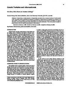
1.5 GAS EXCHANGE TO ASSESS PHOTOSYNTHETIC PERFORMANCE IN PLANTS 1.5.1 A:Ci curves and A:Cc curves Gas exchange can be used to understand the underlying physiology of photosynthesis in plants. Instruments such as the LI-6400XT Portable Photosynthesis system (LI-COR Inc., Lincoln, NE, USA) measure fluxes of CO2 and H2O diffusion through leaf stomata. CO2 is the main substrate for Rubisco in the Calvin Cycle. The difference between CO2 concentration entering and exiting a chamber where the leaf is placed permits calculation of the CO2 assimilation rate by the leaf (A). The LI-COR is able to regulate different CO2 concentrations around the leaf so that CO2 response curves can be measured. Knowing stomatal conductance (gs), the intercellular CO2 concentration (Ci) can be calculated such that A:Ci curves can be constructed (Figure 1.2). Since Rubisco carboxylation rate depends on the partial pressure of CO2 inside the chloroplast (Cc), one also needs to know the mesophyll conductance (gm) in leaves. This allows the construction of A:Cc curves (Figure 1.2). Cc takes into account the resistance to diffusion that CO2 encounters between the intercellular airspaces and the chloroplast stroma as it diffuses through the cell wall membranes and aqueous phase to Rubisco.

27


Figure 1.2 CO2 assimilation rate, A, as a function of intercellular CO2, Ci, (diamonds) and chloroplastic CO2, Cc (circles) at 21% Oxygen, 25 °C. Model curves fitted to A are shown. Data from one flag leaf of Triticum aestivum cv. Mace. Flow rate 500 μmol s-1, irradiance 1800 μmol quanta m-2 s-1. gm was assumed to be 0.55 mol m-2 s-1 bar-1. Transition from Vcmax to J limited curves occurred at A=28.5 μmol CO2 m-2 s-1 (horizontal arrow) and Cc=252 μbar and Ci=324 μbar (vertical arrows).

The response curves can be used to estimate the velocity of carboxylation of Rubisco (Vcmax) and the RuBP regeneration or electron transport rate (J) based on the C3 biochemical model (Farquhar et al., 1980). When net photosynthesis is positive, the intercellular CO2 partial pressure (Ci) is greater than that in the chloroplast (Cc). Using A:Cc curves to calculate Vcmax means that the initial slope is steeper than in A:Ci curves, which changes the range where Rubisco activity or RuBP regeneration are the rate limitation. It is expected that the estimation of Vcmax and J in the leaf will be more realistic by using Cc (Figure 1.2.). A is a commonly measured parameter for assessing photosynthetic performance; it is found to vary among wheat genotypes and has been related to wheat yield (Reynolds et al., 1994; Fischer et al., 1998b; Gutierrez-Rodriguez et al., 2000; Reynolds et al., 2000). However, A is strongly dependent upon gs (Condon et al., 2004). A can be high because the genotype has high biochemical capacity or because it has high gs or a leaf can have high capacity but be measured when gs was low (Figure 1.3). For this reason, Vcmax and J are more robust traits than A to study photosynthetic capacity in plants.

28


Figure 1.3 CO2 assimilation rate, A, depends on stomatal conductance, gs, for a leaf with a certain Vcmax and J. Point (a) has the same A as (b) but with a lower gs and requires a higher Vcmax and J capacity.

1.5.2 Meaning of Vcmax and J Calculations and detailed stoichiometry of Vcmax and J have been widely described in the biochemical model of leaf photosynthesis for C3 plants (Farquhar et al., 1980; von Caemmerer, 2000). The model is based on the Calvin cycle and the electron transport chain taking into account photorespiration and Rubisco kinetics using the MichaelisMenten equation. The biochemical model assumes stoichiometries for carboxylation, oxygenation and electron transport. During carboxylation, one molecule of RuBP yields two molecules of 3phosphoglycerate (PGA). For oxygenation, one molecule of RuBP produces one molecule of PGA and one molecule of 2-phosphoglycolate, which is recycled in the photorespiratory cycle to produce 0.5 molecules of PGA. During thylakoid electron transport, the reduction of NADP+ to NADPH + H+ requires the transfer of two electrons, which in turn requires four photons, two to each photosystem (von Caemmerer, 2000). In the C3 biochemical model of leaf photosynthesis two main equations describe the process: one, the maximum velocity of Rubisco (ribulose-1,5-bisphosphate carboxylaseoxygenase) carboxylation (Vcmax) and two, the electron transport rate (J) needed for RuBP (ribulose-1,5-bisphosphate) regeneration. The response of A at different CO2 partial pressures (C) is used to derive values for the variables Vcmax, J and Rd by assuming values for several Rubisco kinetic parameters (Equations 1.2 and 1.3). 29


𝐴=

𝑽𝒄𝒎𝒂𝒙 (𝐶−Γ∗ ) 𝐶+𝐾𝑐 (1+

𝐴=

𝑱(𝐶−Γ∗ ) 4𝐶+8Γ∗

𝑂 ) 𝐾𝑜

− 𝑅𝑑

− 𝑅𝑑

(1.2)

(1.3)

The equations are based on the Michaelis-Menten equation. For plant leaves it is necessary to consider carboxylation and oxygenation, which requires the O2 partial pressure, O, the Michaelis-Menten constants for CO2 and O2, Kc and Ko respectively, and Γ* that is the chloroplastic CO2 partial pressure at which the rate of carboxylation equals the rate of photorespiratory CO2 release. Because instruments routinely measure net assimilation of CO2, non-photorespiratory CO2 release by mitochondrial respiration (Rd) is also needed. Vcmax and J are key photosynthetic traits for a leaf. In biological terms, Vcmax represents the maximum rate of carboxylation by Rubisco. Figuratively, Vcmax has been compared to the power of a car engine; a car with more cylinders will have a higher capacity and more power. In the case of J, in biological terms, it represents the rate at which energy from the sun is used by the leaf for photosynthesis. J is the electron transport rate which enables the regeneration of RuBP. Sunlight captured by the leaf pigments is converted into chemical energy in the chloroplast splitting H2O molecules which generate electrons that flow through photosystem II and I to produce NADPH and ATP that are used in the regeneration of RuBP in the Calvin Cycle. Continuing the alternative analogue, J can be seen as petrol for a car, the energy that makes the engine to work. Photosynthetic measurements are extensively used to calculate Vcmax and J in plant physiology and ecophysiology. However, a tool that allows a greater number of individuals to be measured for photosynthetic performance is still needed. 1.6 LEAF REFLECTANCE TO ASSESS PHOTOSYNTHETIC PERFORMANCE IN PLANTS Reflection is ‘the redirection of a beam of radiation when it encounters a boundary’. The beam can be reflected coherently as happens with a mirror or can be scattered by unequal surfaces. The beam is electromagnetic radiation, which because of the time spent travelling in magnetic and electric fields can be seen as electromagnetic waves. A wavelength measured in meters is the distance between adjacent wave crests from the electromagnetic wave, and frequency measured in cycles is the number of waves that go across a certain 30


point in one second. Electromagnetic waves from all frequencies form the electromagnetic spectrum (Jones and Vaughan, 2010). Some regions of the spectrum are: Far (vacuum) ultraviolet (UV) (10-180 nm), Near UV (180-350 nm), visible (VIS) (350-770 nm) (Ingle and Crouch, 1988). Photosynthetically Active Radiation is defined from 400 to 700 nm (McCree, 1971). Reflectance from the first part of the electromagnetic spectrum has been related to xanthophylls, chlorophylls, and water in plants (Figure 1.4.a), and the red edge in the derivative of reflectance is commonly related to photosynthesis (Figure 1.4.b) (Peñuelas and Filella, 1998). The IR region is commonly divided in to three bands: near infrared (770-1300), short wave infrared 1 (SWIR1) region (1300-1900 nm), and short wave infrared 2 (SWIR2) region (1900-2500 nm). Research in this part of the spectrum has increased because hyperspectral cameras and radiometers can more easily measure the full spectrum, 350-2500 nm and secondly because the information has been useful. IR spectra measured in leaves have been correlated with photosynthetic parameters (Vcmax and J) (Serbin et al., 2012), and have been used to predict carbon, nitrogen and phosphorus in leaf extracts (Gillon et al., 1999). Other uses are in imaging, for example vision at night (Figure 1.5).

Figure 1.4 Reflectance (a) and the first derivative of reflectance (b) spectra for typical healthy leaves. The main wavelengths used in physiological reflectance indices are indicated: 430 and 445 nm for carotenoids; 531 and 570 nm for xanthophylls; 550–680 nm and `red-edge' position for chlorophyll; 700–800 nm for brown pigments; 800 and 900 nm as structural reference wavelengths; 970 nm for water; and 800–900 nm and 680 nm for green biomass’ (Peñuelas and Filella, 1998).

31


Figure 1.5 The same photo taken during the night using (a) a normal camera (b) using a SWIR camera. http://www.sensorsinc.com/gallery/images.

1.6.1 Measuring reflectance from a canopy Reflection from vegetation has been measured with radiometers and images from satellites for global vegetation programs which began in 1972 with the multi-spectral satellite LANDSAT 1. Reflectance has been used to estimate terrestrial photosynthesis and light use efficiency from vegetation because it is the source of primary production on the planet (Grace et al., 2007). Numerous vegetation indices (VI) using the visible and infrared region of the spectrum have been proposed to measure chlorophyll in vegetation (Zarco-Tejada et al., 2001). The most successful are the photochemical reflectance index (PRI) and the normalized difference vegetation index (NDVI). PRI is correlated with the xanthophyll cycle which protects plants from photodamage, and uses reflectance from the visible region at 531 and 570 nm (Gamon et al., 1992). NDVI is used to track active photosynthesis in the biomass of a plant canopy using reflectance in the visible and infrared region of the electromagnetic spectrum (Tucker, 1979). More recently, measurements of the full spectrum from 350-1000 nm or 350-2500 nm depending on the instrument have been used to estimate leaf chemical properties and leaf dry mass per area (LMA). For instance, high spectral resolution remote sensing from Airborne Visible Infrared Imaging Spectrometer (AVIRIS) has successfully predicted leaf chemical properties and leaf mass per area (LMA) from a tropical forest using the partial least square regression (PLSR) (Asner and Martin, 2008; Asner et al., 2009; Asner et al., 2011a; Asner et al., 2011b). Leaf nitrogen, chlorophyll a and b, carotenoids, LMA and assimilation of CO2 have also been predicted from spectral reflectance at canopy level. Correlations of predictions varied from R2=0.49 for Amax to R2=0.9 for LMA (Doughty et al., 2011).

32


1.6.2 Measuring reflectance from a leaf One advantage of measuring leaf reflectance is that the spectra are not too contaminated by reflectance from the soil and the atmosphere. Both of these factors can complicate the usefulness of canopy reflectance spectra. Leaf measurements are important because they have allowed scaling up to canopy level and provide a link to biochemical measurements in the laboratory. Reflectance measurements of leaves have been reported since 1929. In 1961, a colorimeter with a reflectance attachment was used to measure the percentage of 625 nm light that was reflected. This value showed a high correlation with chlorophyll content in soybean and Valencia orange leaves, thus providing a useful indicator of chlorophyll content in leaves (Benedict and Swidler, 1961). A chlorophyll-meter based on transmittance of 670 and 750 nm, correlated strongly (0.998) with chlorophyll content. Consequently, this method was developed for estimating the deepness of green colour and the chlorophyll content per unit area of the leaves (Inada, 1963). Nowadays, there are several portable leaf chlorophyll meters available in the market, such as the Minolta SPAD chlorophyll meter. SPAD measures the chlorophyll content via light transmittance through absorbance of red light at 650 nm and infrared light 940 nm, it is hand-held battery portable and there is a model that permit to save the information and download in the computer (Mullan and Mullan, 2012). Following from the success of remote sensing at the canopy level, hyperspectral reflectance has been developed for predicting physiological and biochemical leaf parameters at leaf level. Successful predictions of photosynthetic parameters have been obtained for tropical trees, aspen, cotton and soybean (Doughty et al., 2011; Serbin et al., 2012; Ainsworth et al., 2014), and nitrogen content and LMA in wheat (Ecarnot et al., 2013). These examples show the potential of using hyperspectral reflectance (350-2500 nm) to screen wheat for photosynthetic parameters. 1.7 THESIS AIM AND OUTLINE It is now possible to calculate Rubisco activity (Vcmax) and electron transport rate (J) and these can serve as main traits to study photosynthetic diversity in wheat. The first objective was to determine variation in photosynthetic parameters using panels of elite wheat lines. Secondly, as the determination of these parameters is slow, the second objective was to develop a new method using hyperspectral reflectance to predict multiple traits. This thesis is composed of conventional methods and hyperspectral reflectance to study and understand photosynthetic diversity in wheat. The first part is based on the 33


biochemical model of leaf photosynthesis for C3 plants and gas exchange measurements. In Chapter 2, the kinetic constants that are used in the biochemical model were adapted for wheat. In Chapter 3 further understanding of Vcmax and Rubisco content measured in vitro were considered to analyse diversity of Vcmax in four sets of wheat genotypes: two experiments in the glasshouse in Australia, one experiment in the field in Mexico and other experiment in the field in Australia. Among others traits, J, leaf dry mass per unit area and leaf nitrogen were considered in each experiment. Statistical comparisons across wheat genotypes, environments and plant stage were used to understand diversity of the traits measured. The second part of the thesis explores hyperspectral reflectance as a rapid tool to measure photosynthetic traits. Chapter 4 presents the methodology used to measure reflectance in wheat and the analysis of the partial least square regression (PLSR). Validation of the method for Vcmax, J, LMA, Narea, SPAD (as surrogate of chlorophyll content) and chlorophylls is shown in Chapter 5. Chapter 6 gives two examples where the models derived in the validations are used to predict J, LMA and Narea in two new set of elite and landrace wheat genotypes. Finally, Chapter 7 presents a synthesis of the main findings of the thesis and possibilities for future research.

34

CHAPTER 2 Biochemical model of C3 photosynthesis applied to wheat at different temperatures

Temperature controlled cabinet. Research School of Biology. ANU. Canberra, Australia, 2014

Chapter 2 Biochemical model of C3 photosynthesis applied to wheat at different temperatures

35

Chapter 2. Biochemical model of C3 photosynthesis applied to wheat at different temperatures

2.1 ABSTRACT In this study, the effect of temperature on estimating Vcmax25 with the C3 photosynthesis model is analysed for wheat. Plants were evaluated under controlled conditions in a growth cabinet and in the field at different temperatures. In the cabinet, measurements were made in 2 and 21 % O2 to constrain the fitting. The fitting of observed CO2 response curves measured in the cabinet began by assuming some of the kinetic constants. The activation energy (E) for Rd from tobacco was assumed and corroborated from observed data. Then, the initial slope from the CO2 response curve was used to calculate the CO2 compensation point (Γ), from which Γ* was predicted. E for Vcmax for wheat was assumed from the literature. Values for Kc and Ko at 25 °C were assumed from tobacco. Values of E for Kc, Ko and Vomax were found along with values for Vcmax and Rd at 25 °C which minimised two variances, namely Γ* and the assimilation rates measured at low CO2 concentrations across all temperatures and both oxygen concentrations. Several new kinetic constants are proposed for wheat. These constants were tested on CO2 response curves measured on wheat genotypes in the field at different temperatures during the course of a day. The new kinetics constants improved the fitting of curves measured at different temperatures.

2.2 INTRODUCTION The biochemical model of leaf photosynthesis for C3 plants is widely used in plant physiology to calculate the maximum velocity of Rubisco (ribulose-1,5-bisphosphate carboxylase-oxygenase) carboxylation in vivo (Vcmax) and electron transport rate (J) or rate of RuBP (ribulose-1,5-bisphosphate) regeneration (Equations 2.1 and 2.2). The model using kinetic parameters derived from tobacco (Nicotiana tabacum) has been applied to many species measured at 25 °C. To adjust the kinetic parameters to different leaf temperatures, the Arrhenius equation (Equation 2.9) has been used. As CO2 response curves measured in the field for this project were obtained at different leaf temperatures (Figure 2.1), it was deemed necessary to verify that this did not bias the estimated values of Vcmax and J. The temperature range for good photosynthetic performance for cold adapted plants is from 0 to 30 ºC and for warm adapted plants between 15 and 45 ºC (Sage and Kubien, 2007). At the beginning of this project, it was assumed that Vcmax25 could be calculated with the Arrhenius equation from measurements of wheat measured in the field between 20 and 34 ºC. However, it became apparent when analysing repeated measurements on the same leaf through a day that this was not the case.

36

Biochemical model of C3 photosynthesis applied to wheat at different temperatures. Chapter 2

Figure 2.1 Leaf temperature for wheat plants measured in the glasshouse (Aus1 and Aus2) and in the field (Aus3 and Mex). Genotype details are given in Chapter 3. Symbols are the average of the repetitions, and error bars represent the standard error from the same repetitions.

Temperature affects plant performance and photosynthesis in a variety of ways. High temperatures can affect Rubisco, Rubisco activase, Rubisco activation state and membrane fluidity. It has been shown that the catalytic turnover of Rubisco (kcat) from C3 plants increases at least 6 times from 16 to 40 ºC, while the affinity for CO2 decreases (Sage, 2002). When deriving estimates of Vcmax from gas exchange measurements, one requires the kinetic parameters Kc and Ko which are the Michaelis-Menten constants for carboxylation and oxygenation respectively, and Vomax that is the maximum velocity of oxygenation (von Caemmerer, 2000). To account for different leaf temperatures, activation energies for each parameter are also required. Using values and activation energies for Vomax, Kc and Ko from tobacco and Atriplex glabriuscula, predictions of CO2 assimilation rate for Chenopodium album were higher than the observed data, particularly at high CO2 concentrations (Sage, 2002). This suggests that the kinetic constants for C. album may differ from those of tobacco. Therefore, it was concluded that activation energies for Rubisco kinetic constants needed to be derived in order to calculate Vcmax25 from the field measurements of wheat carried out here. Rubisco is a bifunctional enzyme catalysing reactions with both CO2 and O2. In order to assess the oxygenase parameters, CO2 response curves were measured under two O2 concentrations and a range of temperatures for each leaf. Analysis of curves obtained under low O2 (2%) permits us to derive Kc, while curves measured at ambient O2 (21%) reflect the 37


apparent affinity when oxygen is competitively inhibiting the carboxylase (von Caemmerer, 2000). By making measurements under two O2 concentrations, it is possible to derive the temperature responses of both Kc and Ko. Although studies using photosynthetic kinetic parameters have been reported for wheat (Table 2.1), no study provides a complete set of information such as available for tobacco (Bernacchi et al., 2001; Bernacchi et al., 2002). The activation energy for Vcmax in tobacco has been shown to be between 64.8 (Badger and Collatz, 1977) and 65.33 kJ mol-1 (Bernacchi et al., 2001). For wheat, a value of 63 kJ mol-1 was obtained (Evans, 1986) and has been assumed here. The activation energy for respiration in tobacco is 46.39 kJ mol-1 (Bernacchi et al., 2001). However, it is likely that this varies between species (Atkin and Tjoelker, 2003). Consequently, some experiments were carried out to corroborate this value for wheat. Table 2.1 In vitro Michaelis-Menten constants for Rubisco in wheat, triticale, tobacco and rice.

Species

Kc Value at 25°C (μbar)

Ko Value at 25°C (μbar)

Triticum aestivum

335±24

304±30

(Makino et al., 1988)

291±10

194±30

(Cousins et al., 2010)

326±27

271±26

(Carmo-Silva et al., 2010)

308.4±3

328.6±6

(Galmés et al., 2014)

488±12

343±10

(Prins et al., 2016)

Triticale

482±72

305±4

(Prins et al., 2016)

Nicotiana

272.38

165.82

(Bernacchi et al., 2002)

tabacum

259

179

(von Caemmerer et al., 1994)

Oryza sativa

239

266

(Makino et al., 1988)

Reference

E: Activation Energy. Solubility for CO2 of 0.0334 mol (L bar-1) and for O2 of 0.00126 mol (L bar)-1 were used to convert Kc and Ko values from concentrations to partial pressures.

Temperature can also affect the fluidity of membranes and the functioning of protein complexes within them (Sage and Kubien, 2007). The temperature dependence of mesophyll conductance (gm) should also be considered in the calculations of Vcmax and J (Sage and Kubien, 2007). Unlike for tobacco, the temperature response of gm for wheat is modest from 15 ºC to 40 ºC (Equation 2.5) (von Caemmerer and Evans, 2015). Since in vitro Rubisco measurements are laborious, kinetics constants have been derived in vivo using CO2 response curves for tobacco (von Caemmerer et al., 1994; Bernacchi et al., 2001). It was decided to pursue the same approach for wheat measuring CO2 response curves at different temperatures and different O2 concentrations.

38


The main purpose of this chapter is to derive a set of kinetic constants for wheat Rubisco that can be used to fit Equation 2.1 to provide more accurate calculations of Vcmax25 from measurements made under variable temperatures.

2.3 MATERIALS AND METHODS 2.3.1 Experiments and gas exchange measurements Results are organised in two experiments described below: Cabinet and Aus3T. For these experiments, gas exchange was measured on the flag leaf of wheat using a LI-6400XT Portable Photosynthesis system (LI-COR Inc., Lincoln, NE, USA). The air flow rate was 500 μmol s-1 with an irradiance of 1800 μmol quanta m-2 s-1. The CO2 concentration used refers to the inlet gas. a) Cabinet For the Cabinet experiment, three wheat genotypes (Merinda, Espada and Mace) and one triticale genotype (Hawkeye) were chosen from previous experiments where they represented the entire range of variability in photosynthetic efficiency for the genotypes measured (see section 3.4.2.2). The four genotypes were sown on August 11th, 2014. Each genotype was sown in three pots of 5 L with 75:25 loam:vermiculite soil mix containing basal fertilizer and grown in a glasshouse with temperature 25/15 °C (day/night) at CSIRO Black Mountain, Canberra, Australia (-35.271875, 149.113982). Plants emerged on August 18th, 2014 and were thinned to two plants per pot about one week later. Gas exchange was measured on flag leaves from September 25th to October 15th, 2014 when the plants were close to anthesis, GS59-60 (Zadoks et al., 1974). On the morning of the measurement, they were transferred from the glasshouse to a controlled environment cabinet (Thermoline Scientific Model-TRIL/SL) and light intensity 200 μmol quanta m-2 s-1 in the facilities of the Research School of Biology in the Australian National University (ANU), Canberra (-35.277078, 149.116686). Plants were well irrigated before and through the experiment to avoid water stress. Temperature required for each measurement was adjusted in the cabinet and in the leaf temperature mode of the LI-COR that was used to measure CO2 response curves. The initial conditions were 21% O2 concentration, 15 °C leaf temperature and 400 μmol CO2 mol-1. When 2% O2 was used, it was obtained by mixing N2 and O2 using mass flow controllers (Omega Engineering Inc. Stamfort, CT,

39


USA). The LI-COR prompt was set to 2% O2 in order to obtain correct gas exchange calculations. Six plants of Merinda (V34) were measured at 51, 52 and 53 DAE with leaf temperatures of 15, 25, 30, 35 °C. At each temperature, CO2 response curves were measured at 21% and then 2 % O2 using 50, 100, 150, 200, 250 and 400 μmol CO2 mol-1. The lights on the LICOR chamber were turned off after the last CO2 response curve was measured, and dark respiration was recorded 30 minutes later. For two plants, respiration was recorded at decreasing temperatures of 35, 30 and 25 °C. In four plants, it was recorded at decreasing temperatures of 35, 30, 25, 20, 15°C and then at increasing temperatures of 15, 20, 25, 30 and 35 °C at 400 μmol CO2 mol-1 and 21 % O2. Two plants of Espada (V25) were measured at 39 and another plant at 50 DAE with increasing leaf temperatures of 15, 30, 35 °C. At each temperature, CO2 response curves were measured at 21% and then 2 % O2 using 50, 100, 150, 200, 250 and 400 μmol CO2 mol-1. For two plants, dark respiration was recorded after 30 minutes at decreasing temperatures of 35, 25 and 15 °C at 400 μmol CO2 mol-1 and 21 %O2. Five plants of Mace (V32) were measured at 57 and 59 DAE and four plants of Hawkeye (V27) were measured at 58 and 59 DAE. For each leaf, CO2 response curves were measured at leaf temperatures of 15, 20, 25, 30 and 35 °C in 21% O2 and 50, 100, 150, 200, 250, 400, 600, 800, 1000 and 1200 μmol CO2 mol-1. After the last curve, the lights on the LI-COR chamber were turned off, and dark respiration was recorded 30 minutes later at decreasing temperatures of 35, 30 and 25 °C at 400 μmol CO2 mol-1 and 21 % O2. b) Field (Aus3T) Field experiment Aus3 is described in detail in Chapter 3 section 3.3.1 and Table 3.1. In experiment Aus3T, four wheat genotypes: V45, V57, V62 and V66 (Table 3.3) from Aus3 were selected to measure temperature responses of leaf gas exchange on December 17th, 2013 when plants were 75 DAE, and flowering nearly completed, approximately at GS69. The measurements were made on three different plants from one plot of each genotype. Field air temperature was recorded with the head of the LI-COR opened. Block temperature was set to approximate the field air temperature; resulting leaf temperature and block temperature were recorded during the experiment (A1). For each leaf, CO2 response curves were measured using 150, 250, 400, 600, 800 and 1200 μmol CO2 mol-1.

40


2.3.2 Calculations of Vcmax, J and mesophyll conductance Results from the Cabinet experiment were used to derive Rubisco kinetic constants. Therefore, calculations for the gm and adjustments to calculate Rubisco activity (Vcmax) and the electron transport rate (J) will be described during the chapter. For experiment Aus3T, the maximum Rubisco activity at 25 ºC (Vcmax25) and J were calculated using the kinetic constants obtained in this chapter (Table 2.2) and the leaf biochemical model of photosynthesis (Farquhar et al., 1980). The average rate of CO2 assimilation (A) of all genotypes (Experiments: Aus1, Aus2, Aus3 and Mex from Chapter 3) was 25 μmol CO2 m-2 s-1, with a mean intercellular CO2 (Ci) of 260 μmol CO2 mol-1 (A260) when measured under ambient CO2. A260 was interpolated from the line relating CO2 assimilation rate to intercellular CO2 concentrations between 50 and 400 μmol CO2 mol-1 for each leaf and subsequently used to estimate gm (Equation 2.4). 2.3.3 Equations CO2 assimilation rate (A, μmol CO2 m-2 s-1) and the chloroplastic CO2 partial pressure, μmol mol-1 (Cc) are used to build the CO2 response curve (Chapter 1, Figure 1.2). The velocity of carboxylation (Vcmax, μmol CO2 m-2 s-1), is derived from the initial slope which depends on the Michaelis-Menten constants for CO2 and O2 (Kc and Ko μbar and mbar, respectively), the O2 partial pressure (O, 197 mbar) and the chloroplastic CO2 partial pressure at which the rate of carboxylation equals the rate of photorespiratory CO2 release (Γ*, μbar). Rubisco limited CO2 assimilation rate is expressed as 𝐴=

𝑉𝑐𝑚𝑎𝑥 (𝐶𝑐 −Γ∗ ) 𝐶𝑐 +𝐾𝑐 (1+

𝑂 ) 𝐾𝑜

− 𝑅𝑑

(2.1)

where Rd is the mitochondrial respiration (μmol CO2 m-2 s-1) (von Caemmerer, 2000). The second part of the CO2 response curve is used to infer the electron transport rate (J, μmol e- m-2 s-1), expressed as 𝐴=

𝐽(𝐶𝑐 −Γ∗ ) 4𝐶𝑐 +8Γ∗

− 𝑅𝑑

(2.2)

The chloroplastic CO2 partial pressure (Cc, μmol) used in equations (2.1 and 2.2) is derived from the intercellular CO2 partial pressure (Ci, μbar), A and the mesophyll conductance (gm, mol m-2 s-1 bar-1) from the following equation (2.3) 𝐴

𝐶𝐶 = 𝐶𝑖 − g

m

(2.3) 41


To a first approximation, gm varies in direct proportion to photosynthetic capacity (von Caemmerer and Evans, 1991). Therefore, the value assumed for gm for each leaf was derived by linear scaling to the rate of CO2 assimilation at a common Ci of 260 μmol mol-1 (A260) using the following equation: g m = g m,avg ∗

𝐴260

(2.4)

25

Where gm,avg, (0.55 mol m-2 s-1 bar-1) was based on the average of six different plants of triticale variety Hawkeye measured with carbon isotope techniques that combine tunable diode laser spectroscopy and gas exchange (Evans and von Caemmerer, 2013) at CSIRO Black Mountain (0.55 mol m-2 s-1 bar-1, Estavillo et al., – unpublished data). This is similar to other values for wheat (Tazoe et al., 2011; von Caemmerer and Evans, 2015). The value of 25 (μmol CO2 m-2 s-1) on the denominator was the average A from all genotypes at 25 ºC. CO2 response curves were measured at different leaf temperatures. A linear response of gm to leaf temperature (von Caemmerer and Evans, 2015) is given by equation 2.5: g mT = g m,25 (0.0094𝑇 + 0.786)

(2.5)

The chloroplastic CO2 partial pressure at which the rate of carboxylation equals the rate of photorespiratory CO2 release (Γ*, μbar) depends on the ratio of the velocities of oxygenation (Vomax, μmol O2 m-2 s-1) and carboxylation (Vcmax). Γ∗ =

𝑉𝑜𝑚𝑎𝑥 𝐾𝑐 𝑂 2𝑉𝑐𝑚𝑎𝑥 𝐾𝑜

(2.6)

A value of 0.22 was assumed for the ratio Vomax/Vcmax at 25 ºC as has been used in tobacco and wheat (von Caemmerer, 2000; Cousins et al., 2010). The observed CO2 compensation point (Γ) was calculated from a line fitted to the measurements made in 50 and 100 μmol mol-1 inlet CO2 concentrations: (𝐶𝑐100 −𝐶𝑐50 )

Γ = 𝐶𝑐50 − 𝐴50

(𝐴100 −𝐴50 )

(2.7)

This value was used to calculate a value for observed Γ* (Γ*,obs) as follows (von Caemmerer et al., 1994): Γ∗,obs = Γ (1 − 𝑉

𝑅𝑑

𝑐𝑚𝑎𝑥

42

𝐾𝑐 (1+

)−[

𝑂 )𝑅 𝐾𝑜 𝑑

𝑉𝑐𝑚𝑎𝑥

]

(2.8)


The temperature response function used for Kc, Ko, Vcmax, Vomax, Rd, and Γ* is given by: 𝑃 = 𝑃25 𝑒

𝐸(𝑇−25) 𝑅∙298∙(𝑇+273.15)

(

)

(2.9)

where P is the parameter value at leaf temperature T (°C), P25 is the value of the parameter at 25 °C, E is the activation energy (kJ mol-1) and R is the universal gas constant 8.314 J mol-1 K-1. To fit observed data with equation 2.1, six main parameters were used: Rd, Γ*, Vcmax, Kc, Ko and Vomax. The photosynthetic model requires a value at 25 °C (value25) and an activation energy (E) for each parameter. Several values were assumed from the literature: E for Rd 46.39 kJ mol-1 (section 2.4.1.1), value25 for Γ* (Bernacchi et al., 2002), E for Vcmax in wheat of 63 kJ mol-1 (Evans, 1986), value25 for Kc and Ko from tobacco (Bernacchi et al., 2001; Bernacchi et al., 2002) and Vomax/Vcmax at 25 ºC of 0.22 (von Caemmerer, 2000; Cousins et al., 2010). The value of Γ*,obs from Eq. 2.8 provided an additional constraint for the fitting routine by comparing it to Γ*new calculated using Equation 2.6 at each temperature and oxygen condition with Kc, Ko, Vomax and Vcmax adjusted to each temperature with Equation 2.9. During the fitting for each leaf, the value25 of Rubisco capacity (Vcmax25) and respiration (Rd) together with E for Kc and Ko were found.

2.4 RESULTS CO2 response curves at different temperatures were measured under two different O2 concentrations to enable the derivation of Rubisco kinetic parameters for wheat. The first group of experiments was carried out in controlled conditions from which a new set of kinetic constants for wheat was obtained. The second group of experiments were used to validate the kinetic constants using CO2 response curves measured at different temperatures in the field. 2.4.1 Leaf model prediction of in vivo photosynthesis in wheat In order to understand the effect of temperature on the calculations of Vcmax , experiments in the cabinet at 21 and 2% O2 were performed, focused on the initial slope of CO2 response curves. Values of Vcmax and J derived from gas exchange measurements and the model fitted to them depend on photosynthetic kinetic constants that have been assumed in the model. The most frequent kinetic constants used to fit the photosynthetic model have been derived from Atriplex glabriuscula and Nicotiana tabacum (Table 2.2.a and 2.2.b). However, using these kinetic constants, the modelled response did not describe the wheat CO2 response curve observed at different temperatures and oxygen concentrations (Figure 43


2.2.a and 2.2.b.). The observed A measured in vivo with gas exchange did not correspond to predictions made using the model (Equation 2.1 and 2.2) with kinetic constants from Table 2.2.a. Using kinetic constants obtained by Bernacchi, 2001 & 2002 derived from tobacco (Table 2.2.b, Figure 2.2.b), improved the fitting but there were still inconsistences, especially at 2% O2. The fitting was substantially improved by deriving new activation energies (Table 2.2.c, Figure 2.2.c). Table 2.2 The kinetic constants used to model CO2 assimilation rate in Figure 2.2 a, b & c. Kinetic constants/Specie (a) N. tabacum2,4 (b) N. tabacum (c) New A. glabriuscula1 constants Kc

Value at 25°C (μbar) E (kJ mol-1) Ko Value at 25°C (mbar) E (kJ mol-1) Value at 25°C (μbar) Γ* E (kJ mol-1) Vcmax Value at 25°C (μmol m-2 s-1) E (kJ mol-1) Vomax E (kJ mol-1) Value at 25°C (μmol Rd m-2 s-1) E (kJ mol-1) References

272.384

59.41 1792 361 37.434 24.464 134

80.994 165.824 23.724 37.434 24.464 113.9

93.72±2.56

64.81 65.86 1.37

65.33 32.58+ 1.27

635

46.393 1(Badger

for wheat 2724

2592

46.393

166

33.6±5.96 37.746 24.426 117.5

27.1±4.86 1.14 46.393

and Collatz, 1977) 1986) 4(Bernacchi et al., 2002) 6This report, n=6 Caemmerer et al., 1994) E: Activation Energy; +Vomax calculated from Bernacchi et al. (2002) constants. Vcmax and Rd values at 25 °C belong to each plot. 3(Bernacchi et al., 2001)

5(Evans,

2(von

Figure 2.2 CO2 assimilation rate, A, as a function of chloroplastic CO2, Cc, at two different O2 concentrations (Open symbols, 2% O2; Closed symbols 21% O2) and four temperatures (square 15 °C, diamond 25 °C, triangle 30 °C, circle 35 °C). Symbols are the observed A from one leaf of Triticum aestivum cv. Merinda. Lines are the predicted A using each column of kinetic constants from table 2.2. Cc was calculated from Equation 2.3, the assumed value of mesophyll conductance, gm, from Equation 2.4 and the temperature dependence of gm,25 from Equation 2.5. Flow rate 500 μmol s-1, irradiance 1800 μmol quanta m-2 s-1 and 50, 100, 150, 200 and 250 μmol CO2 mol-1 of CO2 reference.

44


2.4.1.1 Kinetic constants for respiration From the literature a similar value of E for Rd has been observed in tobacco and wheat (Evans, 1986; Bernacchi et al., 2001). In order to confirm this, dark respiration (Rdark) in leaves of wheat was measured at 15, 20, 25, 30 & 35 °C and fitted using E= 46.39 kJ mol-1 (Table 2.2). This activation energy derived from Tobacco matches that observed here for wheat dark respiration (Figure 2.3). The temperature response was similar whether obtained with increasing or decreasing temperatures (not shown). We assume the temperature dependency for Rd is the same as that for dark respiration.

Figure 2.3 The temperature response of dark respiration, Rdark, for flag leaves of Triticum aestivum cv. Espada, Hawkeye, Mace and Merinda. Each point is the mean of three to six leaves. The error bars are the standard error from the leaves measured. Each leaf was measured after a CO2 response curve and 30 minutes of darkness, at five temperatures from 15 °C to 35 °C. The line is the predicted respiration from 10 °C to 40 °C using Equation 2.9, E=46.39 kJ mol-1, R=8.314 J mol-1 K-1, Rdark(25 ̊C) = 1.2 μmol CO2 m-2 s-1. Flow rate of 500 μmol s-1 and at 400 μmol CO2 mol-1 for inlet CO2.

2.4.1.2 Kinetic constants for the compensation point Two important points can be extracted from the initial slope of the CO2 response curve: Γ, where the curve crosses the x axis (A = 0), and Γ*, the CO2 partial pressure on the curve when A = -Rd (von Caemmerer, 2000). From the observed CO2 response curves measured on Merinda, at 15 °C, 25 °C, 30 °C and 35 °C, at 21 and 2 % O2 (Figure 2.2.), a line fitted to the first two points was used to calculate Γ (Equation 2.7), and then Γ* observed (Γ*obs) using Equation 2.8, assuming that E of Vcmax in wheat is 63 kJ mol-1 (Evans, 1986), E of Rd is 46.39 kJ mol-1 (section 2.4.1.1), and value25 for Kc and Ko from Bernacchi et al. (2001, 2002). Under 21% O2, the observed CO2 compensation point, Γ, closely matched that observed for tobacco (Figure 2.4.a). However, under 2% O2 the observed Γ was slightly less than that predicted using tobacco Rubisco kinetic parameter values. 45


Figure 2.4 Temperature dependence of the CO2 compensation point in 2 and 21% O2. a) CO2 compensation point when A=0. Circles are the observed Γ derived from six A:Ci curves from flag leaves of Triticum aestivum cv. Merinda (Equation 2.8). Dashed lines are Γ calculated with kinetic constants from Bernacchi et al. 2002 (Equation 2.7). b) CO2 photocompensation point when A= -Rd, the solid lines are Γ*new calculated from the new kinetic constants.

The average value for the CO2 photocompensation point, Γ*new, from six plants of Merinda measured at 21 % O2 and 25 °C was 35.4±0.41 μbar using an atmospheric partial pressure for Canberra of 938 mbar. When adjusted to sea level (oxygen partial pressure 210 mbar), this equates to 37.74 μbar. The value of E for Γ* was obtained by summing E for Vomax and Kc, and subtracting E for Vcmax and Ko after the fitting (24.4 kJ mol-1, Table 2.2.c). This value is similar to that reported for tobacco (Table 2.2.b). Thus, the value and temperature dependence of the CO2 photocompensation point appears to be similar between wheat and tobacco. 2.4.1.3 Fitting observed values in the model Minimising the variance between Γ*obs and Γ*new helped to constrain the solution of the fitting which also tried to minimise the variance between A observed and predicted at each temperature and both oxygen concentrations using Equation 2.1. This procedure was repeated for six different plants of Merinda. The average activation energies for Kc and Ko obtained from Merinda (Table 2.2.c) were then used to fit data collected from other genotypes (Mace, Hawkeye and Espada) at different temperatures in the cabinet to assess their general validity.

46


Figure 2.5 CO2 assimilation rate, A, as a function of chloroplastic CO2, Cc a) and intercellular CO2, Ci b), in 21% oxygen at five different leaf temperatures (Square 15 °C, cross 20 °C, diamond 25 °C, triangle 30 °C, circle 35 °C). Model curves are A predicted with the new kinetic constants in Table 2.2.c. Symbols are the observed A of one flag leaf from Triticum aestivum cv. Mace. Flow rate 500 mol s-1, irradiance 1800 μmol quanta m-2 s-1. Cc was calculated from Equation 2.3.

The ability of the new constants to fit CO2 response curves is illustrated in Figure 2.5. Two versions are shown. The fundamental data obtained from the LI6400 (A:Ci) are shown in panel b), whereas A:Cc curves are shown in panel a) because it was necessary to include gm when fitting Equations 2.1, 2.2, 2.3, 2.4 and 2.5. The initial slope of the CO2 response curves is used to derive Vcmax, which increases at higher temperatures. For example, from A:Cc curves, Vcmax was 50, 78, 121, 184 and 277 μmol CO2 m-2 s-1 at 15, 20, 25, 30, 35 ºC respectively (Figure 2.5). As temperatures increase, the affinity of Rubisco for CO2 decreases such that the initial slope changes little. The increase in respiration rate also contributes to the increase in Γ at higher temperatures. At high CO2 partial pressures, the RuBP regeneration limited rate increased by 30% from 15 to 30 ºC before declining at 35 ºC. The transition from a Rubisco to an RuBP regeneration limitation happens at a lower chloroplastic CO2 partial pressure (230 to 250 μbar) compared to intercellular CO2 partial pressure (240 to 280 μbar), but did not vary greatly with temperature.

2.4.2 Assessing the new kinetics constants for wheat in the field The new parameters (Table 2.2.c) were used to fit A:Cc curves obtained in the field (Aus2T). The model curves could be fitted well to the observed data (one example shown in Figure 2.6). 47


Figure 2.6 CO2 assimilation rate, A, of a wheat leaf (V45) measured in the field as a function of chloroplastic CO2, Cc; a) Full A:Cc curve at 26 and 32 °C; b) Initial slope at different temperatures (diamond 26 °C, asterisk 28 °C, triangle 30 °C, circle 32 °C). The lines predict A with the new kinetic constants of Table 2.2.c. Flow rate 500 μmol s-1, irradiance 1800 μmol quanta m-2 s-1 and 21% O2.

2.4.2.1 Vcmax trends for wheat in the field and in controlled conditions Genotypes measured in Aus3T and in the cabinet were used to assess the validity in estimating Vcmax at 21% oxygen at different temperatures. First, values for Vcmax and Rd were sought that minimised variance between observed and modelled rates predicted using Equation 2.1 with the new kinetic parameters. Vcmax25 was calculated using Equation 2.9 from each curve measured at different leaf temperatures. To avoid possible effects of declining Rubisco activation at temperatures higher than 30 °C, only values derived from leaf temperatures up to 30 °C were used (15 to 30 °C in the cabinet and 25 to 30 °C in Aus3T) to calculate the baseline of 100%. Second, two ways of calculating Vcmax were used and compared: 1. Vcmax fitted using measurements from multiple temperatures and the new kinetic constants: Values for Vcmax25 and Rd were sought by fitting the model at each temperature (15, 20, 25, 30 and 35 °C) using the new kinetic constants (Table 2.2.c), which will be called Vcmax(new). 2. Vcmax fitted at each temperature using Bernacchi constants: Values for Vcmax25 and Rd were sought by fitting the model at each temperature (15, 20, 25, 30 and 35 °C) using tobacco kinetic constants (Table 2.2.b), which will be called Vcmax(Bernacchi). 48


Figure 2.7 Assessing the stability of Vcmax25 estimated for a leaf measured at multiple temperatures either under controlled conditions (cabinet) or the field (Aus3T). Values of Vcmax were derived using the new kinetic constants (closed symbols) or tobacco kinetic constants (Bernacchi et al., 2001; Bernacchi et al., 2002) (open symbols) at each temperature and then converted to Vcmax25 using equation 2.9. Error bars are the standard error from repetitions, which are described in Materials and Methods.

Ideally one should obtain the same value for Vcmax25 regardless of the temperature used during the measurement. The baseline of 100% represented the mean value from curves measured up to and including 30°C. Relative values of Vcmax(new) and Vcmax(Bernacchi) are shown in Figure 2.7. In both cases, the estimate of Vcmax25 tended to decline as measurement temperature increases. However, Vcmax(new) shows less deviation with temperature than Vcmax(Bernacchi) (generally ±5% and ±20%, respectively). The deviations appear to be greater when measured in the field (Aus3T) compared to measurements made in controlled conditions (cabinet). The decreased variation in Vcmax25 using the new constants should improve estimation of Vcmax from field data that in some cases was obtained at leaf temperatures greater than 25 °C. 2.4.2.2 Changes in A, Vcmax and J at different temperatures Leaf temperature affects A, Vcmax and J differently. In the cabinet, A showed a broad peak with a maximum near 20 °C (Figure 2.8.a). By contrast, values for Vcmax and J obtained from A:Cc curves with the new constants show quite strong temperature responses (Figure 2.8.c). J increased from 15 to 30 °C and then decreased, while Vcmax increased up to the maximum temperature measurement, 32 °C in the field and 35 °C in the cabinet. In the field and in the cabinet J and Vcmax crossed over at 30 °C.

49


Figure 2.8 Temperature response of a) CO2 assimilation rate, A, b) A predicted from Vcmax (Wc), Equation 2.1, or J (Wj), Equation 2.2, c) Rubisco carboxylation rate, Vcmax (red) and electron transport rate, J, (blue) calculated with the new constants. Mean of three flag leaves from different plants of Triticum aestivum V45 measured in Aus3T through a day with leaf temperature increasing from 26 to 32 °C (closed symbols). Mean of five flag leaves measured in the cabinet from different plants of T. aestivum cv. Mace with leaf temperature increasing from 15 to 35 °C (open symbols). a) measured when inlet CO2 was 400 μmol CO2 mol-1, b) predicted from chloroplastic CO2 and Equations 2.1 or 2.2, with gm calculated from Equation 2.4, c)Vcmax and J derived from CO2 response curves (Figure 2.5 and 2.6) were used to predict A (Wc and Wj, respectively).

The predicted assimilation rates from A:Cc curves assuming Rubisco or RuBP regeneration limitation (Equations 2.1 and 2.2, respectively) were remarkably similar (Figure 2.8.b), but apparently cross from being Rubisco limited below 30 °C to being RuBP regeneration limited above 30 °C in the cabinet. In the field, A was apparently Rubisco limited between 26 and 32 °C in part because of a reduction in chloroplastic CO2. Both Vcmax and J were greater for field-grown leaves than for leaves from plants grown in the glasshouse for the cabinet measurements. The modelled values for A predicted in Figure 2.8 reflect the observed rates (Figure 2.8.a.) reasonably well.

50


2.5 DISCUSSION The estimate of Vcmax from CO2 response curves depends on the values assumed for the kinetic parameters of Rubisco. As there are few complete sets of values, it is common to assume those determined for tobacco (Bernacchi et al., 2001; Bernacchi et al., 2002). However, it became apparent that using these values from tobacco to analyse wheat measured at different temperatures was problematic. Consequently a detailed characterisation of CO2 response curves measured under a range of temperatures and two oxygen concentrations was undertaken. This chapter highlights the importance of adjusting the biochemical model by using kinetic parameters derived for wheat. The new parameters were compared against repeated photosynthetic measurements across a range of leaf temperatures measured in the field or growth cabinet. The new parameter values improved the ability to derive an estimate of Vcmax from A:Ci curves measured in the field at leaf temperatures other than 25 °C compared to when activation energies from tobacco were assumed. 2.5.1 Rubisco kinetic constants for wheat Some kinetic constants from tobacco calculated in vivo helped to fit observed data for wheat in vivo. In vitro value25 for Kc and Ko in wheat differ from those obtained in vivo in tobacco, mainly for Ko. In vitro Ko for wheat is reported as 304 μbar (Makino et al., 1988) and 328 μbar (Galmés et al., 2014) while value25 of Kc for tobacco is half lower than in vitro values (166 μbar). Reports for Kc and Ko measured in vitro for different species, make it difficult to select the set of value25 and E that should be used in the fittings, and an inadequate choice could result in poor predictions (Table 2.2.a). A common way to derive Vcmax and J is with a published spreadsheet in excel (Sharkey et al., 2007) which uses kinetic constants obtained in vivo from tobacco (Bernacchi et al., 2001; Bernacchi et al., 2002). Previously, value25 had been reported for Kc, Ko, * and kcat based on analysis of CO2 response curves of transgenic tobacco which had reduced Rubisco content (von Caemmerer et al., 1994). The spreadsheet with that set of kinetic constants has been used in most of the higher plants, assuming that all the plants have the same mechanism for CO2 assimilation. In part it is true, since prediction of A at 25, 30 and 35 ºC were acceptable when the kinetic constants from Bernacchi et al., 2001 & 2002 were used to predict observed data from wheat (Table 2.2.b). However, there were some inconsistencies in the fitting that were fixed for wheat. The new E of Kc and Ko for wheat increased and Vomax decreased in comparison with tobacco. We fixed the value of E for Vcmax for wheat at 63 kJ 51


mol-1 (Evans, 1986) which is slightly less than that for tobacco, 65.3 kJ mol-1 (Bernacchi et al., 2001). Perhaps these differences are normal since it has been reported that E for kcatc in vitro varies from 48 to 72 kJ mol-1 across crops (soybean, rice, cotton, tobacco, tomato, spinach, wheat) and E of kcatc in vitro for wheat is higher than for tobacco (Galmes et al., 2015). As well, E of kcatc in vitro from land plants showed a positive correlation with the optimum growth temperature and Rubisco specificity factor (Sc/o) (Galmes et al., 2015). Tobacco is from warmer environments than wheat and the temperature required for optimal growth is higher (25 and 20 ºC, respectively), which could relate to the differences in E of Kc and Ko obtained in this experiment. It is also reported that the specificity factor (Sc/o) in vitro for tobacco is 82 and 107 mol mol1

for wheat (Parry et al., 1989; Whitney et al., 2009). Interestingly, the assumed value25 for

Kc and Ko helped to solve the rest of the kinetic parameters in wheat where Γ* resulted in almost similar values (Table 2.2). Γ* reflects Sc/o in vivo. The discrepancy of Sc/o in vitro and in vivo need more work to understand the two different answers. 2.5.2 Effect of temperature on estimating Vcmax25 Vcmax calculated with the new constants for wheat varied at increasing temperature (15, 20, 25, 30, 35 ºC, Vcmax of 50, 78, 121, 184, 277 μmol CO2 m-2 s-1 respectively, Figure 2.5) and during the day temperatures can vary from 23 to 34 ºC (Figure 2.1), for this reason conversion to value25 (Vcmax) is important analysing Rubisco activity for field measurements. However, measurements at temperature higher than 30 ºC should be reconsidered in wheat because the wheat growth and Rubisco could be affected. The optimum growth temperature in wheat during anthesis and grain filling is 20 ºC and the maximum cardinal temperature (when wheat can recover) is 31 ºC at anthesis and 35.4 ºC during grain filling (Porter and Gawith, 1999). Measuring in the field (experiments Aus3 and Mex) the highest temperatures were during anthesis and grain filling between noon and early afternoon. Short periods of heat may not detrimentally affect wheat plants when grown under good management and with irrigation. Thus it should be possible to obtain Vcmax25 from Vcmax derived at higher temperatures from plants when they are grown under yield potential conditions. However, when high temperatures are expected in the field, it would be better to restrict gas exchange measurements to the morning. In the case of Rubisco, activation state can be affected by CO2 concentrations and temperature. In fitting the model for C3 photosynthesis to calculate Vcmax, a full Rubisco activation state was assumed. However, in sweet potato, it has been shown that the 52


Rubisco activation state varies depending on CO2 concentration. It is higher at low CO2 (Ci=140 μbar) and lower at high CO2 concentrations (Ci=500 μbar). Rubisco activation state also decreased at temperatures above 30 ºC. When measured at ambient CO2 (Ci=250 μbar), activation state decreased from the highest value of 85 % at 30 ºC to 65 % at 40 ºC (Sage and Kubien, 2007). Two ideas can be extracted from this information. First, we may have underestimated Vcmax if Rubisco was not fully activated. Second, plants growing in the field are subjected to variation in temperature. If this altered the activation state of Rubisco, then Vcmax derived from field surveys could be confounded by temperature. For wheat, gm did not increase greatly at higher temperatures (von Caemmerer and Evans, 2015), but the ability of Rubisco to select CO2 over O2 decreases such that photorespiration increases from 25 to 35 ºC (Figure 2.3). It was possible to fit CO2 response curves at 35 ºC to calculate Vcmax25 in wheat and by making measurements under both 2% and 21% O2, we were able to untangle the changes in carboxylation and oxygenation as temperature varied. Nevertheless, measurements from plants that have been exposed to 30 to 35 ºC for a long time need to be used with caution and one needs to be aware that when deriving Rubisco activity, certain assumptions are required. 2.5.3 Effect of temperature in respiration Respiration occurs in the mitochondria, and it is the process by which plants consume O2 and release CO2. Respiration increases with increasing temperature. At temperatures around 5 °C, enzymes have lower maximum catalytic activity and membranes are less flexible, both of which could reduce respiratory flux. At 25°C, enzymatic performance and availability of substrates both increase compared to that at 5°C and membranes are more flexible. These changes help to increase the flux through respiration. However, at higher temperatures, membranes became very fluid, the activity of some enzymes decrease and substrates may become limited, all of which affect the respiration flux (Atkin and Tjoelker, 2003). In Figure 2.3, dark respiration rate per unit leaf area increased with increasing temperature almost doubling from 25 to 35 ºC. Increasing respiration has also been observed for Spinacia oleracea L. cv. Torai grown at 15/10 °C and 30/25 °C (Yamori et al., 2005).

2.6 CONCLUSIONS Vcmax and J are valuable traits to be considered when comparing photosynthetic performance between wheat lines. In this chapter, Rubisco kinetic constants from tobacco were combined with several new kinetic constants appropriate for wheat in order to 53


calculate Vcmax from CO2 response curves measured in the field at different temperatures. The new constants will be useful to reduce environmental error when calculating Vcmax for leaf temperatures ranging from 15 to 35 °C. However, data from plants grown for long periods of heat should be considered separately because Rubisco activation state can decline at high temperature. The new kinetic parameters derived in this chapter provide appropriate values for wheat such that analysis will no longer need to assume values derived from tobacco.

54

CHAPTER 3 Genetic variation for photosynthetic capacity and efficiency in wheat


Chapter 3 GENETIC VARIATION FOR PHOTOSYNTHETIC CAPACITY AND EFFICIENCY IN WHEAT

55

Chapter 3. Genetic variation for photosynthetic capacity and efficiency in wheat

3.1 ABSTRACT This study uses basic physiological mechanisms to understand photosynthetic capacity (Vcmax25 and J) and efficiency (Vcmax25/Narea) in wheat to analyse genotypic diversity in relation to fertilizer, plant stage and environment. Four experiments (Aus1, Aus2, Aus3 and Mex) were carried out to investigate genetic variation for Vcmax25, J, and Vcmax25/Narea in wheat with complementary traits (A, gs, Ci/Ca, LMA and Narea). Genotypes for Aus1 and Aus2 were grown in the glasshouse with two fertilizer levels. Genotypes for Aus3 and Mex experiments were measured in the field in Australia and Mexico respectively; Mex genotypes were measured at two plant stages. Results showed that Vcmax25 and J are robust parameters to assess photosynthetic capacity since they did not depend on gs or grain filling and Vcmax25 was positively correlated with Rubisco measured in vitro. The main nitrogen effect and development stage did not influence the ranking of genotypes for Vcmax25, J and Vcmax25/Narea. However, growing conditions and geographical location affected ranking of the genotypes. There was significant genotypic variation in most of the experiments for Vcmax25, J and Vcmax25/Narea, except for genotypes measured in Mexico.

3.2 INTRODUCTION The efficiency of crop production has been defined in thermodynamic terms as the ratio of energy output (carbohydrate) to energy input (solar radiation), which is given by the slope of the relationship between dry matter production and intercepted radiation (g MJ-1) (Monteith, 1977). This parameter is also termed radiation use efficiency (RUE) and its importance is evident in the link with biomass and yield (Equation 1.1). Evidence from modelling and CO2 enrichment suggests that RUE of wheat could be increased ~50% with improvement in photosynthetic traits (Reynolds et al., 2012b). In the past, assimilation rate (A) has been used to assess photosynthesis in wheat. Some studies have shown diversity in A across wheat genotypes and a positive, minimum or no correlation with yield or with modern wheat genotypes (Murthy et al., 1979; Reynolds et al., 1994; Fischer et al., 1998b; Gutierrez-Rodriguez et al., 2000; Reynolds et al., 2000; Sadras et al., 2012). Two additionally important parameters to assess photosynthetic performance are Rubisco activity (Vcmax) and electron transport rate (J). These parameters can be extracted by modelling the physiological response of leaves to CO2 and light (Farquhar et al., 1980). While these parameters require more than a single point measurement of A, they have proven to be robust traits to assess photosynthetic capacity in C3 plants since they do not depend on stomatal conductance (gs) as is the case for simple measurements of A (Condon et al., 2004). In the last 20 years Vcmax and J have become common parameters used in plant 56

Genetic variation for photosynthetic capacity and efficiency in wheat. Chapter 3

physiology and ecophysiology, probably because of the availability of portable tools to assess A in the field (Long et al., 1996) . However, few papers have been published analysing genetic variation for Vcmax and J in wheat (Driever et al., 2014; Jahan et al., 2014) and these measurements were done in isolation from other important leaf parameters. If we intend to use such derived traits for selecting wheat varieties with high RUE, it is necessary to compile more information about the genotypic variation for Vcmax and J and have a better understanding of these traits. At present there is no published data for wheat analysing genotypic variation for photosynthetic capacity and efficiency using Vcmax and J measured in the field. Leaf nitrogen is also relevant to the study photosynthetic performance because around 30% of leaf nitrogen from a C3 sun plant is invested in CO2 fixation and 23% directly in Rubisco protein (Evans and Seemann, 1989). It has also been observed that while A is positively correlated with leaf nitrogen, there is variation in A for a given leaf nitrogen content (Evans, 1989). These data indicate that higher leaf nitrogen does not always indicate higher photosynthetic capacity. Carboxylation efficiency (carboxylase activity per unit of leaf nitrogen) has been used to detect variation in photosynthetic performance between two Triticum species (Evans and Seemann, 1984). Therefore, it will be useful to analyse Vcmax an indicator of Rubisco activity, as a function on leaf nitrogen per unit area (Vcmax/Narea), which is termed photosynthetic efficiency in this study. This chapter analyses photosynthetic capacity (Pc) defined as the amount of investment in photosynthetic machinery per unit leaf area (i.e.Vcmax and J) when photosynthesis is not limited by water, light or nitrogen, and photosynthetic efficiency (Peff) as the photosynthetic carbon gain in the leaf per unit of nitrogen invested per unit leaf area. The chapter analyses genotypic variation for these metrics of photosynthetic performance from two perspectives. Firstly, analysing photosynthesis from plant physiological and biochemical mechanisms and secondly assessing photosynthetic diversity under different conditions. Determining the physiological mechanisms underlying variation in photosynthetic traits will permit us to understand the relationship between leaf biochemistry and leaf anatomy; in this case by measuring leaf dry mass per unit area (LMA). LMA is the ratio between leaf dry mass and leaf area, and correlates with the leaf lamina thickness. LMA comprises different leaf compounds from non-structural and structural carbohydrates, proteins, lignin, lipids, minerals, organic acids, and the density of epidermal cells and mesophyll cells which contain a large number of chloroplasts. High LMA can be due to a thick leaf and/or high leaf density, and a higher chloroplast area (Poorter et al., 2009). 57


Assessing photosynthetic diversity under different conditions will help to understand Pc and Peff in relation to genotypic variation, plant stage and environment. Complementary measurements such as gs and the ratio of internal to atmospheric CO2 concentration (Ci/Ca) are used here to assess the water exchange in leaves (Evans and von Caemmerer, 1996; Condon et al., 2004). SPAD is used as a rapidly measured non-destructive surrogate for chlorophyll content (Konica Minolta, 2009-2013). In some cases yield component traits were measured to have a better understanding of plant life cycle and phenology as longer duration of photosynthetic activity can also be related to prolonged demand for grain filling (Evans, 1993). The objectives of this chapter are to analyse photosynthetic variation between elite wheat genotypes at the leaf level. Vcmax and J will be evaluated to assess Pc considering A as conventional trait to assess photosynthesis. Vcmax/Narea as a trait to assess Peff will be explored and analysed across different wheat genotypes. Environmental conditions will be tested to understand the factors that influence Pc and Peff across the elite wheat genotypes.

3.3 MATERIALS AND METHODS 3.3.1 Experiments Results were organised in four experiments (Table 3.1). Experiment Aus1 was set up in a glasshouse at CSIRO Black Mountain, Canberra (-35.271875, 149.113982), from March 31st to June 30th 2012, artificial light was used in June to extend the photoperiod to 16 h and temperature was controlled to 25/15 °C (day/night). Two seeds were sown in cylindrical pots of 1.06 L (15 × 5cm) with 75:25 loam:vermiculite containing basal fertilizer, and one plant per pot was kept for the experiment which was organized in a randomized block design, three blocks representing each repetition for the high nitrogen treatment (+N) and other three blocks for the low nitrogen treatment (-N). Extra fertilizer Thrive (~300 mL per pot of 1.77g L-1N:27%, P:5.5%, K:9%) was applied each week for +N treatment until 83 DAE. A severe low nitrogen treatment was obtained irrigating the pots with water without fertilizer 1.5 month before measurements. Plant emergence was on April 8th. 23 days after emergence (DAE) and the flag leaf was measured at anthesis (GS58-69) from 73 to 83 DAE. The collection of plants used in this experiment is called the “early vigour set” and it was measured at anthesis so the acronym used for these data is EVA (“early vigour anthesis”); further information is described in the germplasm section. Six to seven genotypes per day at similar plant stage with three repetitions were measured and sampled. Details of traits are in section 3.3.4. 58

Genetic variation for photosynthetic capacity and efficiency in wheat. Chapter 3 Table 3.1 Details of experiments

Set of genotypes

Description

Key measurements Stage Traits

Aus1 = Glasshouse experiment. CSIRO Black Mountain, Australia (2012) EVA(-N),(+N) 16 genotypes Anthesis A, Vcmax25, J 3 repetitions 73-83 DAE SPAD, Narea Low/high N Aus2 = Glasshouse experiment. CSIRO Black Mountain, Australia (2012) BYPB(-N),(+N)

30 genotypes Pre-anthesis A, Vcmax25, J 2 repetitions 48-56 DAE SPAD, Narea Low/high N Aus3 = Field experiment. GES-CSIRO, Australia (2013)

BYPB

28 genotypes Pre-anthesis A, Vcmax25, J 4 repetitions 46-54 DAE SPAD, Narea EVA 2 genotypes Anthesis A, Vcmax25, J 4 repetitions 62-67 DAE SPAD, Narea CA 21 genotypes Anthesis A, Vcmax25, J 4 repetitions 60-67 DAE SPAD, Narea Mex = Field experiment. CENEB-CIMMYT, Mexico (2012-2013) CB CA

30 genotypes 3 repetitions 30 genotypes 3 repetitions

Pre-anthesis 67-82 DAE Anthesis 88-103DAE

A, Vcmax25, Jg, Jf SPAD, Nmass A, Vcmax25, Jg, Jf SPAD, Nmass, Narea

EV= Early vigour set; BYP= BUNYIP set; C= CIMCOG set. B= before anthesis (pre-anthesis); A= anthesis.

DAE=

Days after emergence. See text for traits abbreviations.

Experiment Aus2 was carried out in a glasshouse at CSIRO Black Mountain, Canberra (35.271875, 149.113982), from October 12th to December 11th 2012, and temperature was controlled to 25/15 °C (day/night). Three seeds were sown in pots of 5 L with 75:25 loam:vermiculite soil mix containing basal fertilizer, and two plants per pot were kept for the experiment which was organized in a randomized block design, two blocks representing each repetition for the high nitrogen treatment (+N) and one block for the low nitrogen treatment (-N). For the +N treatments extra fertilizer Aquasol (~300 mL per pot of 1.77g L-1N:23%, P:4%, K:18%) was applied every three days from 41 days after emergence (DAE) to 56 DAE. Treatment –N was less severe than Aus1, it was obtained irrigating the plants with water without fertilizer 10 days before measurements. Plant emergence was on October 17th and the flag leaf was measured before anthesis (GS49-57) from 48 to 56 DAE. Measurements were done in one plant per pot for +N and in the two plants per for –N. The collection of plants used in this experiment is called BUNYIP and it was measured before anthesis so the acronym used is BYPB. Details of germplasm used 59


are below in section 3.3.2. Six to ten genotypes per day at similar plant stage with two repetitions were measured and sampled. Experiment Aus3 was carried out in the field at CSIRO Experimental Station at Ginninderra (GES), Australia (-35.199837, 149.090898) from September 25th to December 17th, 2013. The emergence of plants was on October 4th, 2013. From 1 to 75 DAE the average maximum from daily temperature (Figure 3.1) was 22.4 °C and the minimum 7.7 °C, in total 142 mm of rain and an accumulative thermal time of 1,126.8 °C. CA and EVA subsets of wheat genotypes were sown in the same experimental design of two randomized blocks. Each block was subdivided into 30 plots (5 × 6). Next to this experimental design, another experimental design of two randomized blocks for the BYPB collection was sown. In this case, each block was subdivided into 42 plots (7 × 6). Each plot for both experimental designs was 5 m × 1.8 m. It contained a single genotype sown in 10 rows, 18 cm apart, and approximately 200 plants m-2. Plots were fertilized and irrigated optimally in all conditions. The BYPB subset of wheat genotypes was measured in the flag leaf before anthesis (GS40-55) from 46-54 DAE where the maximum temperature reached was 28.3 °C and the minimum 5.4 °C. When EVA (GS69, 62-67 DAE) and CA (GS56-69, 60-67 DAE) subset of wheat genotypes were measured, the maximum temperature reached was 32.2 °C and the minimum 4.3 °C. Measurements and sampling were done twice in two plots, resulting in 4 repetitions for 4 to 5 genotypes per day that were at similar plant stage. In this experiment many plants were at the same stage at the same time and fewer wheat genotypes could be measured: 2 wheat genotypes from EVA, 20 wheat genotypes and 6 triticale genotypes from BYPB, and 22 wheat genotypes from CA. They are marked with asterisk in tables 3.2 and 3.3. Details of germplasm used are in section 3.3.2. Experiment Mex was carried out in the field at Centro Experimental Norman E. Borlaug (CENEB) research station, located in the Yaqui Valley, Sonora, Mexico (27.370837, 109.930362) for a winter-spring cycle. The sowing was on November 23rd, 2012 and the harvest on April 30th and May 2nd 2013 (150 and 152 DAE respectively). Plant emergence was on 2nd, December, 2012. From the 1 to 138 DAE, the average maximum temperature from daily temperature (Figure 3.1) was 26 °C and the minimum 8.3 °C, in total 15.38 mm of rain and an accumulative thermal time of 2,364.6 °C. Plants were organised in a randomised 5 × 6 lattice experimental design with three repetitions. Each repetition (10 × 3 plots) enclosed two subdivisions of 5 × 3 plots. Each plot (2.4 m × 8.5 m) contained a single genotype sown in 6 rows, two beds in the middle with two rows each and two beds in the edges with one row of the same genotype, the second row in the edges corresponded 60


to the next genotype or a filling genotype. Beds followed the system 56-24, where 56 cm is the furrow width and 24 cm is the raised bed width. Plants were grown under optimal management in the field. There were in total five auxiliary irrigations, the total 500 mm of water applied. First fertilization was at soil preparation with 50 kg ha-1 of N and 50 kg ha-1 of P and a second fertilization in the first irrigation of 150 kg ha-1 of N. The CB subset of wheat genotypes was measured in the flag leaf before anthesis (GS49-57) from 67 to 82 DAE, where the maximum temperature reached was 29.7 °C and the minimum 1.5 °C. The CA subset of wheat genotypes was measured in the flag leaf at anthesis (GS60-69) from 88 to 103 DAE, where the maximum temperature reached was 32.1 °C and the minimum 2.5 °C. Measurements and sampling were done in one plant per plot; 3 to 6 genotypes per day were measured at similar plant stage with 3 repetitions.

Figure 3.1 Meteorological conditions in Obregon, Mexico and Ginninderra, Australia. Daily observations from days after emergence (DAE) during measurements in Australia (1-75 DAE) and in Mexico (1-38 DAE). Minimum and high temperature in pink, precipitation in blue bars, minimum and maximum humidity (white circles) and solar radiation in red.

61


3.3.2 Germplasm As described three sets of wheat/triticale genotypes were used in these experiments (Table 3.2). Table 3.2 List of wheat genotypes used for early vigour and BUNYIP set. Early Vigour (EV) Type Gen Name BW V1 Bencubbin BW V2 Halberd BW V3 K1056 BW V4 Nacozari BW V5 Oasis BW V6 Sunstar BW V7 W010311 BW *V8 W020308 BW *V9 W100104 BW V10 W130114 BW V11 W170316 BW V12 W210308 BW V13 W610501 BW V14 W650208 Quarrion BW V75 BW Pitic V76

Gen *V15 *V16 *V17 *V18 *V19 *V20 *V21 *V22 *V23 *V24 *V25 V26 *V27 *V28 *V29 *V30

Name Abacus Axe Bogong Bolac Canobolas Caparoi Chopper Derrimut Drysdale Emu Rock Espada H45 Hawkeye Hunter Hyperno Jaywick

BUNYIP (BYP) Type Gen T *V31 BW *V32 T *V33 BW *V34 T *V35 DW *V36 T *V37 BW *V38 BW *V39 BW *V40 BW *V41 BW V42 T V43 BW V44 DW T

Name Kosciusko Mace Magenta Merinda Pastor Scout Speedee Spitfire Super Seri Tahara Weebil Yenda Zebu Zulu

Type T BW BW BW BW BW T BW BW T BW BW BW DW

T, Triticale genotypes. DW, Durum wheat. BW, Bread wheat. *Genotypes measured in the field in Australia (Aus3).

(1) Early Vigour (EV) set consisted of 16 wheat genotypes from CSIRO in Australia. Genotypes from V1 to V6, V75 and V76 have shown differences in photosynthesis in previous experiments and genotypes from V7 to V14 are characterized to have greater embryo, fast leaf area development and low leaf mass area. (2) A subset of the Best and Unreleased Yield Potential (BUNYIP) that contains 21 wheat genotypes and 9 triticale genotypes with high yield in Australia. (3) CIMMYT Core Germplasm (CIMCOG) Subset II has 30 wheat genotypes selected at CIMMYT (International Maize and Wheat Improvement Center) for high yield (Table 3.3). Acronym for BUNYIP will be ‘BYP’, for CIMCOG will be ‘C’ and for Early Vigour will be ‘EV’. An additional letter will be added to each acronym, ‘B’ meaning before anthesis, and ‘A’ meaning anthesis.

62

Genetic variation for photosynthetic capacity and efficiency in wheat. Chapter 3 Table 3.3 List of wheat genotypes used for CIMCOG Subset II. CIMCOG Subset II (C) Gen *V45

Type BW

Name BABAX/LR42//BABAX/3/VORB

V46

BW

BACANORA T 88

*V47

BW

BCN/RIALTO

V48

BW

BECARD/KACHU

V49

BW

BRBT1*2/KIRITATI

*V50

BW

SAUAL/4/CROC_1/AE.SQUARROSA (205)//KAUZ/3/ATTILA/5/SAUAL

V51

BW

SAUAL/WHEAR//SAUAL

*V52

BW

CMH79A.955/4/AGA/3/4*SN64/CNO67//INIA66/5/NAC/6/RIALTO

*V53

WD

CIRNO C 2008

*V54

BW

CNO79//PF70354/MUS/3/PASTOR/4/BAV92*2/5/FH6-1-7

*V55

BW

CROC_1/AE.SQUARROSA(205)//BORL95/3/PRL/SARA//TSI/VEE#5/4/FRET2

V56

BW

KINGBIRD #1//INQALAB 91*2/TUKURU

*V57

BW

MILAN/KAUZ//PRINIA/3/BAV92

V58

BW

PAVON F 76

*V59

BW

PBW343*2/KUKUNA*2//FRTL/PIFED

*V60

BW

PFAU/SERI.1B//AMAD/3/WAXWING

*V61

BW

SERI M 82

*V62

BW

SIETE CERROS T66

*V63

BW

SOKOLL//PBW343*2/KUKUNA/3/ATTILA/PASTOR

*V64

BW

TACUPETO F2001/SAUAL/4/BABAX/LR42//BABAX*2/3/KURUKU

*V65

BW

TACUPETO F2001/BRAMBLING*2//KACHU

*V66

BW

TC870344/GUI//TEMPORALERA M 87/AGR/3/2*WBLL1

*V67

BW

*V68

BW

*V69

BW

V70

BW

*V71

BW

*V72

BW

TRAP#1/BOW/3/VEE/PJN//2*TUI/4/BAV92/RAYON/5/KACHU UP2338*2/4/SNI/TRAP#1/3/KAUZ*2/TRAP//KAUZ/5/MILAN/KAUZ// CHIL/CHUM18/6/UP2338*2/4/SNI/TRAP#1/3/KAUZ*2/TRAP//KAUZ BECARD WBLL1*2/KURUKU*2/5/REH/HARE//2*BCN/3/CROC_1/AE.SQUARROSA(213) //PGO/4/HUITES YAV_3/SCO//JO69/CRA/3/YAV79/4/AE.SQUARROSA(498)/5/LINE1073/6/ KAUZ*2/4/CAR//KAL/BB/3/NAC/5/KAUZ/7/KRONSTAD F2004/8/KAUZ /PASTOR//PBW343 BECARD

*V73

BW

KFA/3/PFAU/WEAVER//BRAMBLING/4/PFAU/WEAVER*2//BRAMBLING

V74

BW

WBLL1*2/4/BABAX/LR42//BABAX/3/BABAX/LR42//BABAX

T, Triticale genotypes. DW, Durum wheat. BW, Bread wheat. *Genotypes measured in Australia (Aus3).

3.3.3 Developmental stages The Zadoks scale was used to describe the growth stages (GS) of wheat (Zadoks et al., 1974). The first day after emergence (DAE) is considered at GS10, when at least 50% of the seedlings showed the first lamina in the soil surface. Here, before anthesis (B) or preanthesis refers to booting and heading stage between GS41-57. After anthesis (A) refers to Anthesis +7 days sampling, this stage is important because the spike reaches the maximum dry weight, the grain weight is insignificant and the water soluble carbohydrate reserves in stem are at their peak (Pask, 2012). In some cases measurements at anthesis were done at 63


the end of heading and up to 10 days after anthesis between GS56-69. In the experiments section, GS details are specified for each experiment. 3.3.4 Traits measured Gas exchange was measured with a LICOR LI-6400XT infrared gas analyser (LI-COR Inc., Lincoln, NE, USA); the 6 cm2 rectangular head was used for experiments Aus1, Aus2 and Aus3, and the 2 cm2 circular head from the fluorescence head (Li-6400-40; LI-COR Inc.) for the Mex experiment. Gas exchange was used to measure the photosynthetic rate at 400 inlet μmol CO2 mol-1 (A), stomatal conductance (gs), the of internal to atmospheric CO2 concentration (Ci/Ca ) and CO2 response curves to obtain the maximum Rubisco activity at 25 ºC (Vcmax25) and the electron transport rate (J or Jg). Vcmax25 and J were calculated, using the kinetic constants obtained in Chapter 2 and the leaf biochemical model of photosynthesis (Farquhar et al., 1980). In Mex experiments, electron transport rate (Jf) was measured with the fluorescence chamber at 400 inlet μmol CO2 mol-1. SPAD-502 chlorophyll meter (Minolta Camera Co., Ltd, Japan) was used as a surrogate for chlorophyll content (Mullan and Mullan, 2012) to measure flag leaves. Flag leaves measured for gas exchange experiments Aus1, Aus2 and Aus3 were sampled three centimetres up and down from the chamber to determine leaf mass area and nitrogen content. Area of the leaf samples was calculated from a digital photo using the program ImageJ 1.47v. Samples were dried then for 48h at 70°C and weighed to obtain leaf mass area (LMA, g m-2). Nitrogen concentration, Nmass (N mg g-1) was determined on the same samples by flow injection analysis (QuikChem® Method, Lachat Instruments, CO. USA) after the Kjeldahl digestion of leaves at the Australian National University (ANU). For Mex experiments, a complete flag leaf was measured using a leaf area meter (LI3050A/4; LICOR, Lincoln, NE), then, dried for 48h at 70°C and weighed to obtain leaf mass area (LMA, g m-2). Nitrogen concentration, Nmass (N mg g-1) was determined at CIMMYT Batan, Mexico with the Technicon AutoAnalyzer II method, where samples are digested and analysed in the Technicon AutoAnalyzer (Galicia et al., 2008). Nmass and LMA were used to calculate nitrogen per leaf area Narea (N g m-2). Rubisco content in vitro was measured for genotypes Espada, Merinda, Mace, Drysdale and Hawkeye measured in the cabinet (see Chapter 2), Aus2 and Aus3 experiments. Immediately following gas exchange measurements, the piece of leaf that was in the LI6400XT chamber was frozen in liquid nitrogen and stored at -80 °C for later determination of Rubisco content. Rubisco content in vitro was quantified from frozen leaf samples. About 0.25 cm2 of leaf tissue was ground in a Ten Broek homogenizer in 1 mL of ice-cold 64


extraction buffer (50mM Epps-NaOH pH 8.0, 1mM EDTA, 1%(w/v) PVPP, 10mM MgCl2, 10mM NaHCO3, 10mM 1M DTT, 0.01% Triton) with 5μL of plant protease inhibitor cocktail Sigma, and centrifuged at 17,000g for 5 min at 4 °C. 25μL of the supernatant liquid plus 75μL extraction buffer were mixed and incubated with 1μL 14Clabelled carboxy arabinitol-1,5-bisphosphate (CABP) at room temperature. After more than 30 min, [14C]CABP bound to Rubisco was separated from free [14C]CABP using gel filtration through 0.7 × 27 cm columns of Sephadex G-50 fine, equilibrated with 20 mM Bicine-NaOH buffer, pH 8, containing 75 mM NaCl. Fractions with Rubisco-CABP complexes were collected and [14C]CABP was determined by liquid scintillation using a Liquid Scintillation Analyzer, Tri-Carb 2800TR from Perkin Elmer. Vcmax25/Narea was used to represent photosynthetic efficiency (Peff). A, Vcmax25 and J were used to represent photosynthetic capacity (Pc). LMA, Nmass, Narea and SPAD were used to understand leaf structure. 3.3.5 Gas exchange measurements details The flow rate in the CO2 chamber of the Li-Cor was set at 500 μmol s-1 for the 6 cm2 head and 350 μmol s-1 for the 2 cm2 head, irradiance at 1800 μmol quanta m-2 s-1, and block temperature at 25 °C. However, at high temperatures, it was difficult to control temperature resulting in higher leaf temperature. Full CO2 response curves were measured in all experiments. The inlet CO2 was modified each experiment depending on the place and conditions of measurements, since there was a trade-off of time and the number of points to use to increase the accuracy of the fitting. In some cases a higher inlet CO2 was used to get saturation levels. The inlet CO2 for each experiment is underline below: o EVA-Aus1: 50, 100, 250, 400, 800 μmol CO2 mol-1. o BYPB-Aus2: 50, 100, 250, 400, 800 μmol CO2 mol-1. o CB-Mex: 50, 150, 400, 800 μmol CO2 mol-1. o CA-Mex: 50, 100, 250, 400, 600, 800 μmol CO2 mol-1. o BYPB-Aus3: 50, 100, 250, 400, 800 μmol CO2 mol-1. o EVA and CA-Field-Aus3: 50, 150, 250, 400, 600, 800, 1200 μmol CO2 mol-1. Mesophyll conductance (gm) was based on the average of 6 different plants from the triticale Hawkeye measured with carbon isotope techniques that combine tunable diode laser spectroscopy and gas exchange at CSIRO Black Mountain, resulting in 0.55 mol m-2 s1

bar-1 (Estavillo et al., – unpublished data). This value also agrees with measurements done

in wheat genotypes (von Caemmerer and Evans, 2014). 0.55 mol m-2 s-1 bar-1 was divided 65


by the average of assimilation rate of all genotypes measured in all experiments (Aus1, Aus2, Aus3 and Mex), A=25 μmol CO2 m-2 s-1, which corresponded to Ci = 260 μmol CO2 mol-1 and to the 400 inlet μmol CO2 mol-1. In order to know A at intracellular CO2 (Ci) of 260 μmol CO2 mol-1 (A260) for each CO2 response curve a linear regression from 50 to 400 inlet μmol CO2 mol-1 for was used. The final formula used is: gm= (0.55/25)*A260 (Details in Chapter 2). 3.3.6 Yield components Yield components were measured in the experiment Mex after wheat physiological maturity following CIMMYT protocols (Pietragalla and Pask, 2012). Yield (Mg ha-1) was calculated from a subsample of grain harvested in 4.8 m2 and dried. Harvest Index, HI is the ratio of grain dry weight from 100 spikes and the total plant dry weight. Biomass at maturity BMM (Mg ha-1) was calculated from HI/Yield. Biomass at flowering, BMF (Mg ha-1) was obtained from dry biomass sampled in 4.8 m2 when plants were flowering, GS6162. Growth Rate, GR (g m-2 day-1) is calculated as the difference between the dry biomass after anthesis (GS61+7 days) and the dry biomass before anthesis (GS41), divided by the days from this period, because gas exchange measurements were made during this period. Biomass was sampled using plants from 50 cm transects from four furrows of two beds in the middle of the plot (0.8 m2). Days to flowering (DTF) are the number of days after seedlings emergence at flowering, GS61-62. Percentage Grain Filling, PGF (%) = (DTM-DTF)/DTM *100. DTM is he number of days after seedlings emergence to physiological maturity. Physiological maturity is considered at GS87 when the grain reaches the maximum dry weight and it becomes viable. 3.3.7 Statistical analysis The analysis of variance (ANOVA), Tukey’s HSD test and the Pearson correlations for phenotypic correlations were carried out with the package Agricolae in R statistical software, version 3.1.3 (2015-03-09) (de Mendiburu, 2015). Pearson correlations were calculated from the mean of each genotype (Tables 3.9, 3.11, A6, A8, A10).

66


3.4 RESULTS 3.4.1 Experimental overview This section shows the ranges of traits measured in four experiments, Aus1, Aus2, Aus3 and Mex (Figure 3.2, Figures A2-A3, see section 3.3.1). The data will be used to analyse photosynthetic capacity and efficiency, starting with the basic leaf mechanisms in photosynthesis, and then analysing leaf-photosynthetic diversity for each set of wheat genotypes, EVA, BUNYIP and CIMCOG.

Figure 3.2 Experimental overview. A, gs, Ci/Ca, Vcmax25, J, Vcmax25/Narea , SPAD, Narea and LMA in Early vigour set, EV (pink); BUNYIP set, BYP (purple); and CIMCOG set, C (blue) grown in different environments and measured at different stages as described in Table 3.1. Boxplots represent the distribution of the data. The coloured section is the interquartile range (IQR), representing 50% of the data. The lower IQR edge is the point at 25% of the data. The middle black point is the mean and the line the median. The upper IQR edge is the 75% point. The whiskers are 1.5 times IQR, showing the minimum and maximum data. Blue circles are outliers.

67


3.4.2

Mechanistic understanding of photosynthesis in wheat

The velocity of carboxylation (Vcmax) represents Rubisco activity in vivo inferred from nondestructive measurements on living plants, but it can also be measured in vitro from leaf samples. Rubisco is present in leaves as an abundant component of chloroplasts and chloroplast and Rubisco account for a high percentage of leaf nitrogen. Anatomical parameters such as leaf mass per unit dry area (LMA) can reflect high leaf density/thickness and higher chloroplast area. For this reason, in this section Rubisco in vivo and Rubisco in vitro are analysed as a function of LMA and nitrogen per leaf area (Narea).

3.4.2.1 Rubisco in vivo When LMA and Vcmax25 were compared across genotypes, a large range for Vcmax25 was observed over a relatively small range of LMA (Figure 3.3.a). Plants grown with low nitrogen (EVA -N_Aus1) seemed to have similar leaf density/thickness as the high nitrogen treatment (EVA +N_Aus1). Similar behaviour was observed for BYPB -N_Aus2 and BYPB +N_Aus2. These observations raise the question of whether Rubisco measured in vitro behaves similarly at high and low fertilizer treatment.

Figure 3.3 Vcmax25 as a function of a) leaf mass area (LMA), and b) nitrogen (Narea) for wheat genotypes grown in different environments and measured at different stages as described in Table 3.1. Symbols represent means of each genotype. The arrow represents the diversity of Vcmax25 for a given LMA or Narea.

68


At low leaf N, there was a positive correlation between Vcmax25 and Narea, but at higher nitrogen content the correlation was low, which suggests that there is significant variability in Vcmax25 for a given nitrogen investment at high leaf nitrogen contents per unit leaf area (Figure 3.3.b). Potentially, this parameter, Vcmax25/Narea, could be used to uncouple measurements of Vcmax25 from leaf nitrogen, and this trait is used to explore photosynthetic efficiency (Peff) across wheat genotypes. 3.4.2.2 Rubisco in vitro Four wheat genotypes and one triticale genotype from the BYPB set were selected based on Peff (Vcmax25/Narea) to measure leaf Rubisco in vitro (by the CABP binding assay). Genotypes from EVA and BYPB were ranked based on the mean of repetitions. For the BYPB set, the means were considered from genotypes measured in the glasshouse (Aus2) and field (Aus3) (Figure 3.4).

Figure 3.4 Diversity of photosynthetic efficiency represented by Vcmax25/Narea of the early vigour set (EVA +N_Aus1) and BUNYIP Set measured in the glasshouse (BYPB +N_Aus2) and in the field (BYPB_Aus3). Genotypes labelled were selected for Rubisco in vitro measurements of Rubisco. Genotypes were ranked based on the mean of repetitions. For the BYPB set, the means were considered from genotypes measured in the glasshouse (Aus2) and field (Aus3).

69


The BYPB set was measured in the cabinet (see Chapter 2), in the glasshouse with two levels of nitrogen (Aus2), and in the field (Aus3) so genotypes from this set were chosen to measure leaf Rubisco in vitro. The genotypes (Espada, Merinda, Mace, Drysdale and Hawkeye) were selected to cover the range between EVA and BYPB, from lower to higher Vcmax25/Narea (Figure 3.4). Measurements of Rubisco in vitro (CABP binding) were compared to Rubisco in vivo (Vcmax25) and related to LMA and Narea using leaf samples from genotypes measured in the growth cabinet, glasshouse, and field. Vcmax25 showed a positive relationship with Rubisco in vitro although it was not directly proportional. Consequently, Vcmax25 per Rubisco declined as Rubisco content per unit leaf area increased (Figure 3.5). Results of this experiment show that LMA did not correlate with the Rubisco content in vitro. Rubisco content varied almost threefold while LMA varied between 45.8 to 65 g m-2 (Figure 3.6.a). This confirms the relationship within a given experiment already shown in Figure 3.3.a. Leaf nitrogen showed a positive correlation with Rubisco in vitro and diversity for a given Narea (Figure 3.6.b), in general similar to Vcmax25 (Figure 3.3.b).

Figure 3.5 Maximum carboxylation rate in-vivo (Vcmax25) as a function of leaf Rubisco content. Genotypes sampled in the cabinet, glasshouse and field, n=41. The shaded band indicates the level of uncertainty of the regression line.

70


Figure 3.6 Leaf Rubisco content as a function of a. leaf mass area (LMA), b. leaf nitrogen per area (Narea). Data from four wheat genotypes and a triticale measured and sampled in the cabinet, glasshouse and field, n=41.

From Vcmax25, representing the carboxylation of Rubisco in vivo, and Rubisco catalytic sites in vitro representing Rubisco content, it is possible to calculate the catalytic turnover rate for Rubisco carboxylation (kcatc). This is shown for each genotype in relation to the leaf nitrogen content (Figure 3.7). Even if these five genotypes represent the extremes from EVA and BYPB set, it was difficult to distinguish genetic diversity for kcatc. Overall, kcatc was not affected by fertilizer treatment. However, kcatc was reduced in Espada samples from fertilized compared to unfertilized plants and when comparing kcatc in relation to leaf nitrogen, Espada, Mace and Merinda showed a tendency for kcatc to decrease at higher Narea. Drysdale and Hawkeye showed no trend with Narea.

Figure 3.7 Catalytic turnover rate of Rubisco carboxylation (kcatc) as a function of nitrogen per leaf area (Narea) in four wheat genotypes and a triticale (Hawkeye). Black dot are plants without fertilizer. Blue dots are plants with fertilizer. Samples from plants grown in the glasshouse or in the field are not differentiated. Dotted line is tobacco kcatc 3.5 mol CO2(molsites)-1s-1 at 25 °C in vivo (von Caemmerer, 2000).

71


In summary both in vivo and in vitro measurements of Rubisco showed that Rubisco is not correlated with LMA. This indicates that anatomical constraints have flexibility to enable significant variation in Rubisco content. Regardless of whether Rubisco was derived from gas exchange measurements (Figure 3.3.b) or quantified in vitro (Figure 3.6.b). Rubisco is strongly related with leaf nitrogen. It seems that there is variation in Rubisco activity per unit leaf nitrogen Vcmax25/Narea that can be exploited. Vcmax25/Narea can be used as one measure of photosynthetic efficiency. However, no evident differences in kcatc were detected across 5 genotypes selected on the basis variation in Vcmax25/Narea. 3.4.3 Genetic diversity in wheat photosynthesis This section evaluate genetic diversity in wheat photosynthesis at leaf level and the factors (plant stage, nitrogen, and environment) that influence photosynthetic diversity across genotypes. Because the focus of this project was to analyse genetic variation for photosynthetic performance, this section is divided by the sets of genotypes measured: Early Vigour set, BUNYIP and then CIMCOG. 3.4.3.1 Early vigour set wheat genotypes (EVA) Half of this germplasm set are wheat genotypes selected for early vigour and the other half are elite wheat genotypes. In this section we are interested in determining if there is diversity in photosynthetic traits across early vigour genotypes and elite genotypes, and if strong fertilizer treatment in the glasshouse affects photosynthetic performance. Nitrogen treatment had a highly significant effect on all variables measured (Table 3.4). The unfertilized treatment reduced A, gs, Vcmax25, J, Narea, SPAD and LMA while Vcmax25/Narea and Ci/Ca increased. Most of the traits were significantly different across genotypes in the ANOVA, and they were also analysed with Tukey’s HSD test (A5). Interaction G × N was not significant for gas exchange derived traits, but G × E was significant for LMA, Narea and SPAD (Table 3.4). For experiment Aus1, A correlated positively with gs, Vcmax25, J, Narea, SPAD and LMA , so that genotypes with high photosynthetic rates had a high maximum velocity of carboxylation, electron transport rate, nitrogen content, chlorophyll content and leaf mass area. Numerous positive correlations were observed among them e.g. Vcmax25 correlated positively with J, Narea, SPAD and LMA (A6).

72

Genetic variation for photosynthetic capacity and efficiency in wheat. Chapter 3 Table 3.4 EVA set, experiment Aus1. Means from 16 wheat genotypes and 3 repetitions per nitrogen treatment, ANOVA residual standard error (SE) with DF=15. Coefficient of variation percentage (CV%). Traits Means ANOVA P-value -N +N SE CV% Genotype Nitrogen G × N A (μmol CO2 m-2 s-1) 11.8 22.6 4 23 0.04 ≤0.001 0.3 gs (mol H2O m-2 s-1) 0.3 0.46 0.12 32 0.04 ≤0.001 0.4 Ci/Ca 0.8 0.74 0.04 4.6 0.06 ≤0.001 0.2 (μmol CO2 mol air-1) Vcmax25 (μmol CO2 m-2 s-1) 62 127 20.6 21.6 0.03 ≤0.001 0.4 J (μmol e- m-2 s-1) 94 188 28.7 20.3 0.04 ≤0.001 0.1 Vcmax25/Narea 74.6 60.2 13 19.3 0.02 ≤0.001 0.8 -2 -1 -1 (μmol m s (gN )) Narea (N g m-2) 0.84 2.1 0.25 16.7 ≤0.001 ≤0.001 0.05 SPAD 26.6 43.9 4.8 13.7 0.002 ≤0.001 0.005 LMA (g m-2) 39.9 42.9 4.4 10.6 ≤0.001 0.002 0.08

3.4.3.2 BUNYIP wheat genotypes (BYPB) BUNYIP wheat genotypes are characterized by very high yield in Australia, but some genotypes have not been released as varieties due to other deleterious traits. The objective of this experiment is to find out if there is variation in photosynthetic traits and related traits to photosynthesis in elite wheat genotypes for Australia. In this case BYPB was evaluated twice: one with a fertilizer treatment in the glasshouse, and second measurements from high fertilizer treatment in the glasshouse were compared with the same genotypes grown in the field. 3.4.3.2.1 Effect of fertilizer in BYPB genotypes –N and +N treatments were less radical than with the Aus1 experiment in order to generate a medium range of photosynthetic and related parameters. Significant effects of fertilizer treatment on genotypes were still detected in all variables except for gs (Table 3.5). –N treatment reduced A, Vcmax25, J, Narea, SPAD and LMA, and increased Vcmax25/Narea. Ci/Ca was similar in both nitrogen treatments. Interaction of G × N was not significant for any trait. As with Aus1, A correlated positively with gs, Vcmax25 and J, so that genotypes with high photosynthetic rate had a high maximum velocity of carboxylation and electron transport rate. J was positively correlated with Narea and Vcmax25 (A8).

73

Chapter 3. Genetic variation for photosynthetic capacity and efficiency in wheat Table 3.5 BYPB set, experiment Aus2. Means from 21 wheat and 9 triticale genotypes with 2 repetitions per nitrogen treatment with standard deviation (SD) and coefficient of variation percentage (CV%). ANOVA degrees of freedom =29. Traits Means ANOVA P-value -N +N SE CV% Genotype Nitrogen G × N A (μmol CO2 m-2 s-1) 26.7 30 2.24 7.9 0.003 ≤0.001 0.1 0.71 0.72 0.16 22 0.09 0.5 0.3 gs (mol H2O m-2 s-1) Ci/Ca 0.78 0.76 0.03 4.6 0.2 ≤0.001 0.5 (μmol CO2 mol air-1) Vcmax25 (μmol CO2 m-2 s-1) 133 160 14.2 9.7 0.04 ≤0.001 0.5 J (μmol e- m-2 s-1) 190 219 15.3 7.5 ≤0.001 ≤0.001 0.2 Vcmax25/Narea 67 58 5.6 9 ≤0.001 ≤0.001 0.2 (μmol m-2 s-1(gN-1)) Narea (N g m-2) 2 2.8 0.18 7.7 ≤0.001 ≤0.001 0.1 SPAD 48.2 51.3 2.7 5.5 ≤0.001 ≤0.001 0.9 LMA (g m-2) 51 54.7 2.9 5.4 ≤0.001 ≤0.001 0.1

3.4.3.2.2 Comparison of BYPB genotypes measured in glasshouse and field Experiments in the field are important since they are close to the real world environment for wheat production, in a canopy with unconstrained root growth. In order to compare the effect on plant behaviour growing in pots in a glasshouse and in the field, the BUNYIP set was measured in the field (Aus3) and compared with the same wheat genotypes grown and measured in the glasshouse (+N Aus2). Significant differences in the effects of growing environment were detected for most of the variables. J and LMA were higher in the field than in the glasshouse. A, gs and Ci/Ca were lower in the field. Vcmax25, Vcmax25/Narea, Narea and SPAD were similar in both environments (Table 3.6.). All traits showed significant differences across genotypes, when analysed with Tukey’s HSD test (A9). G × E interaction was significant for gs, Ci/Ca , Vcmax25 , J, Vcmax25/Narea and LMA. Table 3.6 BYPB set measured in glasshouse (+N_Aus2) and in the field (Aus3). Means from 17 wheat and 9 triticale genotypes, 2 repetitions in +N_Aus2 and 4 repetitions in Aus3. ANOVA residual standard error (SE) with DF=25. Coefficient of variation (CV%). Traits Means ANOVA P-value +N_Aus2 Aus3 SE CV% Genotype Env G×E A (μmol CO2 m-2 s-1) 30.1 27.3 2.6 9 ≤0.001 ≤0.001 0.1 0.72 0.46 0.14 25.8 0.05 ≤0.001 0.003 gs (mol H2O m-2 s-1) Ci/Ca 0.76 0.68 0.05 6.5 0.05 ≤0.001 0.001 (μmol CO2 mol air-1) Vcmax25 (μmol CO2 m-2 s-1) 161 165 16 9.7 ≤0.001 0.15 0.004 J (μmol e- m-2 s-1) 221 246 17.3 7.3 ≤0.001 ≤0.001 0.004 Vcmax25/Narea 57.8 58.3 7 12.2 ≤0.001 0.7 0.002 (μmol m-2 s-1(gN-1)) Narea (N g m-2) 2.8 2.9 0.25 8.9 ≤0.001 0.26 0.2 SPAD 51.4 52.4 2.65 5 ≤0.001 0.01 0.4 LMA (g m-2) 55 63.4 3.7 6 ≤0.001 ≤0.001 0.004

74


When there is a significant G × E interaction, it is important to make one correlation for each environment to see if any trait has a different behaviour at given environment. Despite G × E being significantly different, one correlation including measurements in glasshouse and field could explain the trend of correlations between traits. A correlated positively with gs, Ci/Ca , Vcmax25, J and Narea, so genotypes with high photosynthetic rate had high gs, intercellular CO2, velocity of carboxylation, electron transport rate and nitrogen content. Vcmax25 and J correlated positively with Narea (A10). 3.4.3.3 CIMCOG wheat genotypes (C) CIMCOG wheat genotypes are elite genotypes from CIMMYT. Two experiments were carried out to evaluate photosynthetic diversity for the CIMCOG set. One analysed the plant stages, before anthesis (CB) and at anthesis (CA) from genotypes grown in the field in Mexico. The second analysed the same genotypes grown in the field in Mexico and in Australia at anthesis. Because usually there is interest in the relationship between photosynthetic traits and yield components, some yield components traits were included in the former experiment. 3.4.3.3.1 Effect of development stage from CIMCOG genotypes The CIMCOG subset of wheat genotypes were compared when measured in the field before anthesis (CB_Mex) and at anthesis (CA_Mex). Plant stage had a significant effect on A, gs, Vcmax25 and SPAD. A, gs, Vcmax25 and Jg had higher values before anthesis than at anthesis. In contrast, SPAD values were lower before anthesis than at anthesis. Ci/Ca, Jg (electron transport rate from gas exchange), Jf (electron transport rate from fluorescence) and Nmass were similar in the two plant stages. Unfortunately, LMA data are missing in this experiment so Vcmax25/Narea was not calculated. There were highly significant differences across genotypes for A, gs, Ci/Ca, Jg, SPAD and for the yield components. However, Vcmax25, Jf, and Nmass were not significant (Table 3.7). Significant traits between genotypes in the ANOVA test were analysed with Tukey’s HSD test (A11). G × E interaction was not significant for any trait. The CIMCOG panel is the only set of wheat genotypes where growing traits and yield components were measured. The analysis of variance showed that there were significant differences across genotypes for all the traits (Table 3.8). The Tukey’s HSD test show the ranking of genotypes (A11 and A12).

75

Chapter 3. Genetic variation for photosynthetic capacity and efficiency in wheat Table 3.7 CIMCOG set measured before anthesis (CB_ Mex) and after anthesis (CA_Mex). The mean is calculated from 30 wheat genotypes and 3 repetitions. ANOVA-Lattice residual standard error (SE) with DF=29. Coefficient of variation (CV%). Traits Mean P-value CB CA SE CV% Gen Stage G × S A (μmol CO2 m-2 s-1) 31.5 27.5 3.7 12.8 ≤0.001 ≤0.001 0.3 0.42 0.36 0.1 28.0 ≤0.001 0.003 0.6 gs (mol H2O m-2 s-1) Ci/Ca 0.6 0.6 0.06 9.3 ≤0.001 0.8 0.6 (μmol CO2 mol air-1) Vcmax25 (μmol CO2 m-2 s-1) 249 189 41.5 18.9 0.4 ≤0.001 0.8 Jg (μmol e- m-2 s-1) 278 276 24.6 8.9 0.03 0.1 0.2 Jf (μmol e- m-2 s-1) 231 225 36.0 15.6 0.7 0.6 0.2 Nmass (mg g-1) 41 42.2 4.8 11.4 0.4 0.2 0.4 SPAD 46.2 50 2.2 4.5 ≤0.001 ≤0.001 0.6 Vcmax25/Narea 69.7 0.35 (μmol m-2 s-1(gN-1)) Jg: electron transport rate from gas exchange; Jf: electron transport rate from fluorescence Table 3.8 Growing traits and yield components of CIMCOG set (Mex). The mean is calculated from 30 wheat genotypes and 3 repetitions. ANOVA-Lattice residual standard error (SE) with DF=29. Traits Mex SE P-value Gen Growth Rate, GR 19.3 5.1 0.05 (g m-2 per day) Days to flowering (DTF) 86.5 1.3 ≤0.001 Biomass at flowering, BMF (Mg ha-1) 9.4 1 ≤0.001 Percentage Grain Filling, PGF (%) 33.1 1 ≤0.001 Biomass at maturity, BMM (Mg ha-1) 14 0.069 0.003 Yield (Mg ha-1) 6.98 0.32 ≤0.001 Harvest Index, HI 0.5 0.014 ≤0.001

A correlated positively with gs, Ci/Ca, Vcmax25 and Jg (Table 3.9). From yield components, A, gs and Ci/Ca had a positive correlation with percentage of grain filling (PGF), but negative correlation with biomass at flowering (BMF) and days to flowering (DTF), so genotypes with high photosynthetic rate, gs and intercellular CO2 had a longer period of time to fill the grain, faster flowering and less biomass at flowering. Interestingly, unlike A, Vcmax25 was not influenced by flowering time as A did. Electron transport rate from gas exchange, Jg, correlated positively with growth rate (GR), but not electron transport rate from fluorescence, Jf. GR had a positive correlation between Nmass, so plants that grew faster before anthesis to anthesis accumulated more nitrogen. Yield did not correlate with any variable, but HI correlated positively with SPAD.

76

Genetic variation for photosynthetic capacity and efficiency in wheat. Chapter 3 Table 3.9 Phenotypic correlation between traits from CB_ Mex and CA_Mex. Traits with significant correlations: ***P≤ 0.001; **P≤ 0.01; *P≤ 0.06. DF=28. Ci/Ca Vcmax25 Jg Jf Nmass SPAD gs A 0.92*** 0.79*** 0.55** 0.47** -0.02 -0.32 0.13 1.00 0.94*** 0.26 0.18 0.03 -0.36* 0.19 gs Ci/Ca 1.00 0.03 -0.06 0.07 -0.38* 0.11 Vcmax25 1.00 0.82*** -0.31 -0.12 0.04 Jg 1.00 -0.14 0.20 0.12 Jf 1.00 -0.03 -0.17 Nmass 1.00 0.07 SPAD 1.00 Yield components GR DTF BMF PGF BMM Yield HI A 0.08 -0.76*** -0.61*** 0.64*** -0.08 -0.10 -0.03 -0.13 -0.81*** -0.69*** 0.75*** -0.07 -0.11 -0.07 gs Ci/Ca -0.23 -0.77*** -0.60*** 0.68*** -0.12 -0.26 -0.20 Vcmax25 0.34 0.18 -0.21 0.22 -0.09 0.10 0.24 Jg 0.46* 0.01 -0.23 0.08 -0.09 0.22 0.39 Jf -0.18 0.08 -0.25 -0.18 0.05 0.01 0.05 Nmass 0.37* 0.49* 0.26 -0.33 0.15 0.26 0.17 SPAD 0.31 -0.28 -0.35 0.32 -0.15 0.18 0.40*

3.4.3.3.2 Comparison of CIMCOG genotypes measured in the field in Australia and in Mexico Experiment Aus3 and Mex provide an opportunity to assess the effect of geographical location on photosynthetic performance in wheat. The ANOVA table shows that the location and genotypes were significantly different for all traits. Genotypes were ranked using Tukey’s HSD test (A13). A, Vcmax25, J, Vcmax25/Narea were higher in genotypes measured in Mexico (CA_Mex) than in genotypes measured in Australia (CA_Aus3). In contrast, Narea, SPAD and LMA were higher in CA_Aus3. The G × E interaction was significant for all traits except for Narea and SPAD (Table 3.10). Table 3.10 CIMCOG set, experiments Aus3 and Mex. Mean from 20 wheat genotypes, 4 repetitions for Aus3 and 3 repetitions for Mex. ANOVA residual standard error (SE) with DF=19. Coefficient of variation (CV%). Variable Means ANOVA P-value Aus3 Mex SE CV% Genotype Env G×E -2 -1 A (μmol CO2 m s ) 24 28 3.8 14.7 ≤0.001 ≤0.001 ≤0.001 0.39 0.38 0.1 27.9 ≤0.001 0.04 ≤0.001 gs (mol H2O m-2 s-1) Ci/Ca 0.67 0.64 0.05 7.4 ≤0.001 ≤0.001 ≤0.001 (μmol CO2 mol air-1) Vcmax25 (μmol CO2 m-2 s-1) 148 188 20.7 12.7 ≤0.001 ≤0.001 0.02 J (μmol e- m-2 s-1) 230 274 26.4 10.7 ≤0.001 ≤0.001 0.008 Vcmax25/Narea 43.5 68.8 6.9 13.1 ≤0.001 ≤0.001 0.003 -2 -1 -1 (μmol m s (gN )) Narea (N g m-2) 3.4 2.7 0.3 8.8 ≤0.001 ≤0.001 0.3 SPAD 55.8 49.8 2.6 4.9 ≤0.001 ≤0.001 0.7 LMA (g m-2) 75 65 4.3 6 ≤0.001 ≤0.001 0.006

77


G × E was significant for most of the traits, for this reason two phenotypic correlations were used to understand the relationship between traits in each location. The main differences found in the two locations were the correlations from LMA, Narea, Vcmax25 and J. In Mex, LMA and Narea were negatively correlated with A and gs but not significant in Aus3. LMA was positively correlated with SPAD in Aus3 but not in Mex. Vcmax25 and J had a positive correlation with gs in Aus3 but not in Mex, and the correlation between Vcmax25 or J with A was stronger in Aus3 than in Mex (Table 3.11). Table 3.11 Phenotypic correlation between traits from CA_ Aus3 and CA_Mex. P-value ≤0.05.Traits with significant correlations: ***P≤ 0.001; **P≤ 0.01; *P≤ 0.06. DF=18. CA_Aus3 Ci/Ca Vcmax25 J Narea SPAD LMA gs A 0.91*** 0.80*** 0.84*** 0.72*** -0.32 -0.13 -0.19 1.00 0.94*** 0.61** 0.43* -0.28 0.04 -0.06 gs Ci/Ca 1.00 0.38 0.20 -0.28 -0.03 -0.10 Vcmax25 1.00 0.91*** -0.18 -0.12 -0.21 J 1.00 -0.25 -0.31 -0.25 Narea 1.00 0.36 0.59** SPAD 1.00 0.60** CA_Mex Ci/Ca Vcmax25 J Narea SPAD LMA gs A 0.94*** 0.79*** 0.52* 0.55* -0.45* 0.03 -0.53* 1.00 0.94*** 0.34 0.33 -0.47* -0.08 -0.56** gs Ci/Ca 1.00 0.16 0.12 -0.41 -0.12 -0.54* Vcmax25 1.00 0.92*** 0.34 0.23 0.19 J 1.00 0.28 0.29 0.10 Narea 1.00 0.18 0.85*** SPAD 1.00 0.12

In summary, there was no significant G × E interaction for fertilizer treatment or for plant stage of development. However, there was G × E interaction when glasshouse vs field, and Australia vs Mexico were compared. Photosynthetic rate was correlated with short flowering time, a longer period of grain filling and reduced biomass at flowering in the CIMCOG set. There was variation for photosynthetic parameters in the Early Vigour, BUNYIP and CIMCOG sets measured in Australia, but there were not always highly significant differences between genotypes. There was no statistical difference across genotypes of the CIMCOG set for Vcmax25 was measured in Mexico.

3.5 DISCUSSION In general there was significant genetic variation for photosynthetic traits across the genotypes measured, parameters considering that all these genotypes are high yielding wheats. Since the main focus of this project was to analyse genotypic variation for photosynthetic capacity and efficiency, this discussion addresses: A. the mechanisms 78


responsible for the ranking of wheat genotypes; B. the bases for the small genotypic variation for Vcmax25 in the Mexico experiments, C. the trends in photosynthetic efficiency measured in Australia and Mexico and finally D. a general reflection on how to scale up from low level traits to yield. 3.5.1 Factors that did not affect the ranking of genotypes for photosynthetic capacity and efficiency Two external factors did not change the ranking of genotypes for the photosynthetic traits: The fertilizer treatments and the plant development stage. There was no interaction between genotypes and fertilizer treatments for A, Vcmax25, J and Vcmax25/Narea (Table 3.4 and 3.5), despite the observation that nitrogen can strongly influence these traits. In this project +N increased A, Vcmax25 and J and conversely –N reduced these values, which agrees with previous observations in wheat where A increases at higher nitrogen contents until a plateau is reached (Evans, 1983). Field experiments in the literature agree with the absence of genotype × nitrogen interaction observed here. It has been suggested that favourable nutrition, particularly nitrogen commonly applied during breeding, will indirectly apply a selection pressure for high photosynthesis and leaf area as a result of the maximum crop growth rate (Richards, 2000). In this project, there was no interaction between genotypes and development stage (G × S) for A, Vcmax25, J and Vcmax25/Narea (Table 3.7). In measurements reported for A in the field at Tlaltizapán, Mexico, significant low G × S (P≤0.02) was observed in 16 wheat cultivars, and the interaction (G × S) did not affect the ranking of the genotypes (Reynolds et al., 2000). In the current experiment A and Vcmax25 were higher before anthesis, GS49-57 (CB_Mex) than after anthesis, GS60-69 (CA_Mex) (Table 3.7). Although measurements from the Tlaltizapán experiment were made at an earlier stage, A was also higher in booting (GS37-49) than in anthesis (GS55-70) (Reynolds et al., 2000). Similar observations have been reported for wheat at the Yaqui Valley, Mexico where A tended to be higher before anthesis (GS39-62) than at anthesis (GS71-77) (Fischer et al., 1998a). It is known that environmental conditions can influence plant energy conversion efficiency (Slattery et al., 2013), and usually temperature is higher after anthesis than before anthesis during the growth cycle of wheat growing in the field. The maximum temperature when CB_Mex was measured was 29.7 C and for CA_Mex this was 32.1 C (Figure 3.1). However, Ci/Ca was similar in the two developmental stages (Table 3.7) and plants that showed low stomatal conductance were remove from the analysis. Solar irradiance was higher when CA_Mex was measured than when CB_Mex was measured (Figure 3.1), probably A and 79


Vcmax25 were lower after anthesis than before anthesis because after anthesis the solar energy was dissipated into heat for photoprotection to maintain the photochemistry (Baker, 2008), Jg and Jf were not significant different by plant stage (Table 3.7), but CO2 assimilation and Rubisco activity was compromised. After anthesis wheat plants start to reallocate assimilates for the future grains, the plant is larger and requires more assimilates to continue growing spikes for other tillers, shoots and roots (Lupton, 1966; King et al., 1967). Low A and Vcmax25 after anthesis than before anthesis can be also due to the compromise of the source and sink relationship, translocation of sugars, hormones and other factors (Wardlaw and Moncur, 1976). Interestingly, there were not significant interaction between CB_Mex and CA_Mex and ranking of genotypes at both plant stages seem to be relatively similar. These observations suggest that while attention needs to be paid to developmental stage and nutrition treatment of material when screening for photosynthetic traits, ranking may be relatively robust across a range of stages and nitrogen levels. 3.5.2 Factors that affected the ranking of genotypes for photosynthetic capacity and efficiency There was significant G × E interaction for Vcmax25, J and Vcmax25/Narea when glasshouse vs field were compared (Table 3.6). However, when Vcmax25/Narea was plotted using the mean of both glasshouse and field measurements, it was possible to differentiate genotypes with higher and lower Vcmax25/Narea (Figure 3.4). One phenotypic correlation table could explain both environment conditions (A10). In this experiment, although some data from the glasshouse can be translated in to the field, it is still important to be aware that ranking of genotypes may change due to environment. J and LMA were significantly different for G × E interaction (E: glasshouse vs field) and both traits were reduced when were measured in the glasshouse (Table 3.6). Possibly some genotypes were affected by the lower light intensity in the glasshouse which is generally lower than in the field due to light absorption, but also from being grown at a different time of the year. Sun leaves are thicker than shaded leaves (Terashima et al., 2006) and LMA is commonly affected by growth irradiance. Plants grown in the field have more light which may lead to increased chloroplast surface area, chlorophyll and Rubisco content and consequently greater photosynthetic capacity (Nishio et al., 1993; Evans et al., 1999). When measuring different sets of genotypes to determine variation in electron transport rate and leaf structure, it is important to take into account such G × E interaction, because genetic 80


potential for J and LMA measured in the glasshouse could be underestimated and as mentioned before, more measurements in the field are required to understand plant physiology (Slattery et al., 2013). There was also G × E interaction for A, Vcmax25, J and Vcmax25/Narea when Australia vs Mexico were compared (Table 3.10). This is not surprising and literature reports on 13 wheat genotypes analysed for A showed significant variation between different locations (Sadras et al., 2012). When the two phenotypic correlations (CA_Aus3 and CA_Mex) were separated, it was possible to observe three main aspects: 1) A had a lower correlation with Vcmax25 and J in Mexico than in Australia (Table 3.11). 2) In Mexico, Vcmax25 measured in the CIMCOG set did not show diversity across wheat genotypes but there was diversity for A and Jg (Table 3.7). Moreover, there was genetic variation for Vcmax25 for the CIMCOG Set in Australia. 3) In Mexico LMA and Narea were negatively correlated with A (Table 3.11, CA_Mex). This behaviour and the environmental drivers responsible of this variation are discussed in the next section. 3.5.3 Understanding photosynthetic performance measured at different geographical locations In order to further explore the differences between A/Vcmax25 correlation measured in Australia (0.84) and in Mexico (0.52) (Table 3.11), all data were re-plotted (Figure 3.8). Immediately, two factors become obvious which could underpin the poor correlation between A and Vcmax25 for genotypes measured in Mexico.

Figure 3.8 Assimilation rate (A) as a function of velocity of carboxylation (Vcmax25) for wheat genotypes grown in different environments and measured at different stages as described in Table 3.1. Symbols are the mean of the traits. Circles delimit the general behaviour of CB_Mex and CA_Mex wheat genotypes.

81


First, genotypes measured before anthesis (CB_Mex) had a higher variation in Vcmax25 for a small range of A (Figure 3.8, symbol “×”). As suggested in the literature, A depends on stomatal sensitivity and this is the reason Ci/Ca has been used to select water-use efficient wheat genotypes (Condon et al., 2004). The present study supports this relationship, where gs was highly correlated with A in all experiments (Table 3.12). For experiments in Mexico, the mean of Ci/Ca was 0.6 (Table 3.7) and in general correlated positively with A (Table 3.12). In the plot (Figure 3.8) it can also be seen that some genotypes with low A had high Vcmax25. This could be explained by some genotypes displaying low A caused by stomatal closure, while in reality their Rubisco capacity was higher, as evidenced by high Vcmax25. This could explain the low correlation between A and Vcmax25 for CB, CA_Mex (Table 3.12). Table 3.12 Summary of phenotypic correlations with photosynthetic rate (A). Taken from genotypic means from Tables A6, A8, A10, 3.9 and A13. Aus1 Aus2 +NAus2 &Aus3 CA_Aus3 CA_Mex CB, CA_Mex

gs

Ci/Ca

Vcmax25

J

0.84*** 0.64*** 0.83*** 0.91*** 0.94*** 0.92***

-0.04 0.21 0.4* 0.80*** 0.79*** 0.79***

0.97*** 0.90*** 0.82*** 0.84*** 0.52* 0.55**

0.92*** 0.79*** 0.87*** 0.72*** 0.55* 0.47**

Second, genotypes measured at anthesis (CA_Mex) had higher variation in A for a small range of Vcmax25 (Figure 3.8). This leads to the same explanation from CB_Mex. Genotypes with low A closed their stomata, inferred from their low gs, but it does not mean that these leaves had lower Rubisco capacity. This confirms that Vcmax25 is not as sensitive to gs as a simple measurement of A and it is a more robust trait to assess Rubisco capacity, as has been suggested decades ago (Farquhar and Sharkey, 1982). Probably this issue of stomatal limitation is more evident during anthesis than before anthesis because temperature was higher after anthesis (Figure 2.1), and even if the plants were grown under potential yield, measurements in the afternoon and high temperatures caused stomatal closure. The utility of Vcmax25 as a metric for Pc is also supported by the strong correlation between Vcmax25 and Rubisco measured in vitro (Figure 3.5). Perhaps the question that needs further attention is why Vcmax25 and Rubisco in vitro have a curvilinear trend (Figure 3.5). In Mexico, Vcmax25 did not show significant diversity across wheat genotypes but there was diversity for J and A (Table 3.7). It is possible that the Mexican environment in which these lines were selected and then measured did not permit expression of genetic variation in Vcmax25 or Rubisco levels. This could be to nitrogen leaching that has been reported in that region, because 75% of the nitrogen fertilizer is applied before planting that can be lost 82


in the first post-planting irrigation (Riley et al., 2001). If there was not enough nitrogen in the soil for plant development, perhaps it was not enough nitrogen allocated to leaves, avoiding the maximum quantity of Rubisco protein into leaves and grain (Hawkesford 2013). However, under these conditions, it seems that there is scope for genetic variation in the electron transport rate (Jg) (Table 3.7). A was also positively related with short flowering time and longer period of grain filling (Table 3.9), which could be related to sink strength. It has been shown that A changes relatively rapidly depending on the demand from grain filling, and A can drop when sink activity from vegetative growth shows before grains start to grow (King et al., 1967; Evans and Dunstone, 1970; Evans, 1993). In these experiments (CA_Aus and CA_Mex) A was measured 7 to 10 days after anthesis. Some genotypes may have started grain filling earlier than others potentially leading to differences in A due to sink demand. Therefore, while A was representative of the photosynthetically active leaves in a given period from anthesis to grain filling, it may not represent the general genetic potential for photosynthetic capacity, as assessed by Vcmax25. Further research is needed to understand the relationship between Vcmax25 and sink strength. There was significant genetic variation for Vcmax25 measured in the CIMCOG Set in Australia. The genotypes were not as vigorous as in Mexico, even if it was attempted to grow the plants under high yield potential conditions; during anthesis temperatures were high, conditions that limited the maximum plant development and could affect expression of maximum Rubisco carboxylation for all genotypes. In regard to potential environmental differences, Mexico belongs to wheat megaenvironment 1 and Australia to wheat megaenvironment 4 (Fischer et al., 2014). Potentially, these genotypes may have reacted to differences in environmental factors such as photoperiod or light intensity (which are the main differences between the two geographical locations) giving more scope for expression of genotypic diversity in photosynthetic traits in Australia. Differences in photoperiod were observed during wheat selection to increase wheat yield from the middle of Mexico to the north of Mexico (Borlaug, 2007). Solar radiation was higher in Australia than in Mexico (Figure 3.1). Perhaps, such differences influenced changes in leaf size, thickness and leaf nitrogen content. Interestingly Narea, LMA and SPAD were lower for genotypes grown in Mexico (CA_Mex) than in Australia (CA_Aus3). Probably different trade-off between leaf structure and photosynthetic traits occurred. For example, in some plants, electron transport is reduced under low irradiance, but it is compensated by investing of more nitrogen in pigment 83


protein complexes (Evans, 1989). Also in an experiment comparing a low and a high level of nitrogen nutrition in spinach, at the highest nitrogen level there was an increase of electron transport capacity despite maintaining the same proportion (24%) of thylakoid nitrogen compared to the low nitrogen treatment, and the excess of nitrogen from the high nitrogen treatment was allocated to the soluble protein (Terashima and Evans, 1988). Plants were bigger with larger leaf area evident in Mexico compared to Australia (unfortunately leaf size was not measured in both locations). Perhaps in Mexico, genotypes had a larger leaf area surface that compensated for a thinner leaf. Having a thin leaf may have limited the chlorophyll and nitrogen per unit leaf area basis. In contrast, plants in Australia increased chloroplast surface with higher LMA to compensate the reduction of leaf size, allowing higher Narea, but it was not enough to increase Rubisco activity. 3.5.4 Understanding photosynthetic efficiency Photosynthetic efficiency, Vcmax25/Narea, was higher in Mexico than in Australia (Figure 3.9). As mention before, wheat genotypes grown in Mexico had a larger leaf area surface than those grown in Australia. Probably, environmental conditions (Figure 3.1) and management resulted in larger leaves and hence in less nitrogen and chlorophyll per leaf area (Table 3.10). Potentially, leaf plasticity may have reacted to environmental conditions and PY management that allowed higher Vcmax25/Narea in Mexico than in Australia. These results showed that 20% reduction in Narea and 10% reduction in SPAD of Mex genotypes in relation to Aus3 genotypes did not penalise photosynthetic capacity. Perhaps, bigger leaves which were more transparent allowed more light go through the canopy. Further experiments regarding photosynthetic capacity and efficiency in the canopy level would be necessary in the future to avoid the limitations of measuring a single organ of the plant, as has been shown in soybean. In soybean(Glycine max L.), a near-isogenic line Clarky11 has approximately 30% lower chlorophyll content than the wild-type Clark but similar CO2 assimilation rate per unit leaf area. It was suggested that canopy CO2 assimilation rate was higher in Clarky11 than Clark because photosynthetic photon flux could penetrate better in the canopy (Pettigrew et al., 1989). However, the greater chlorophyll reduction will inevitably decrease A. Scaling of Vcmax and photosynthetic efficiency can be confounded by pleiotropic effects that will affect the conversion efficiency for biomass and yield (Slattery, 2014).

84


Figure 3.9 Diversity for photosynthetic efficiency (Vcmax25/Narea) from wheat genotypes of CIMCOG set measured at anthesis in Mexico (CA_Mex) and Australia (CA_Aus3). Symbols are the mean of the repetition, the error bar the standard error. Genotypes are ranked from the mean of each genotype including both environments (Aus3 and Mex).

Four Triticum aestivum and one of the Triticale genotypes from the BYPB set selected to cover a range of 46 genotypes for Vcmax25/Narea (Figure 3.4) showed similar catalytic turnover rate of Rubisco carboxylation (kcat) (Figure 3.7). Perhaps variation was minimised because Vcmax was normalized to 25 °C. Genotypic variation was more apparent in different Triticeae species when measurements were done at 35 °C than 25 °C (Prins et al., 2014). The parameter Vcmax25/Narea was found to be a good way to evaluate carboxylation efficiency as was proposed previously (Evans and Seemann, 1984). It could facilitate the selection of plants with higher Vcmax25 without requiring an increase in leaf nitrogen and also normalizes for leaf age related differences in N. 3.5.5 Scaling up from low level traits to yield In this study, reversing the “reductionist” approach in order to scale up (Passioura, 2010) showed no correlation between photosynthetic traits and yield or HI (Table 3.9). This is similar to early research when A was compared with yield across modern high-yielding cultivars (Brinkman and Frey, 1978; Hart et al., 1978; Murthy and Singh, 1979; Gifford and 85


Evans, 1981; Evans, 1993; Sadras et al., 2012). Possible reasons why scaling up from flag leaf photosynthesis to yield seem to fail are: 1) Too few measurements. A correlated with yield when A was measured often (Reynolds et al., 1994; Fischer et al., 1998b; Gutierrez-Rodriguez et al., 2000; Reynolds et al., 2000). The A:Ci curves used to calculate Vcmax25 and J take a long time to measure with gas exchange. Consequently, in this research only one or two measurements were done in the plant cycle. More frequent measurements in more leaves during the plant cycle are probably necessary to determine the accumulated assimilate and this should potentially be compared with plant biomass as a first approximation of assimilates use in the plant. 2) Time of measurements. Consideration should be given to the developmental stage when the measurement of Vcmax25 and J are most likely to influence yield. For wheat grown under optimal conditions, photosynthesis may be more important from 1015 days before flowering because this is the period when the steam is growing, the grain number is set and the most of the florets are growing (Fischer, 1985). Further analysis should be done for Vcmax25 and J over a diurnal cycle, and over the course of longer periods during growth to see weather spot measurements can be related over a day, a week or weeks of measurements. 3) Canopy photosynthesis and remobilisation from other sinks (such as stems) were ignored. In this research, spot measurements were made in the upper most flag leaf. Thus, no account was made for photosynthesis from the spike, from lower leaves, for variation in leaf area, on leaf area duration or in canopy stature. It has been shown that wheat spikes make an important contribution to assimilate supply during grain filling (Sanchez-Bragado et al., 2014) and that remobilisation of carbohydrates stored in the stem pre-anthesis also plays a key role in grain filling (Asseng and van Herwaarden, 2003). 4) Photosynthesis from source tissue could be used differently in each genotype. Photosynthesis is the sole source of energy to plants for growing roots, stems, leaves, spikes and grains (King et al., 1967). However, each wheat genotype may have different sink demands and in this research it was unknown exactly how assimilates were used by the plant: i.e. in respiration, dissipation via heat, growth and development or temporary storage. 5) Yield is the product of LI, RUE and HI (Equation 1.1). Photosynthesis is related to RUE but LI and HI can also be major drivers of yield and were not uniform across all genotypes analysed here. HI, the ratio between grain and biomass, has been a 86


major breeding target for yield and even if there is increased availability of source carbon (i.e. biomass), but the grain sink is low, yield will not be correlated with photosynthetic capacity due to lack of optimisation of partitioning. Source-sink relationships need to be take into account since crops may be either source or sink limited across different developmental stages and during grain filling (Rawson et al., 1976; Reynolds et al., 2005).

3.6 CONCLUSIONS Vcmax25, J and Vcmax25/Narea are shown here to be robust traits with which to assess genotypic variation in photosynthetic performance in wheat; they are not highly influenced by gs or by sink strength during grain filling. Vcmax25/Narea can be used to select for photosynthetic efficiency, since Vcmax25/Narea normalizes Rubisco activity for leaf nitrogen content that can vary with leaf age and nitrogen availability and split the clustering observed when only Vcmax25 is used. While statistically significant differences across genotypes were not always found for photosynthetic traits, sufficient diversity in photosynthetic capacity and efficiency was found. In general, nitrogen applications and plant stage did not change the ranking of genotypes. However, environmental conditions can modify plant plasticity and photosynthetic traits. Understanding and exploiting photosynthetic variation in plants is still challenging given our inability to currently monitor daily photosynthetic performance in plants during the whole plant cycle, in multiple leaves or in a complete canopy in field conditions. Rapid methods to assess photosynthetic parameters are still required.

87


88

CHAPTER 4 Can reflectance spectra be used to predict photosynthetic characters in wheat?


Chapter 4 CAN REFLECTANCE SPECTRA BE USED TO PREDICT PHOTOSYNTHETIC HARACTERS IN WHEAT?

89

Chapter 4. Can reflectance spectra be used to predict photosynthetic characters in wheat?

4.1 ABSTRACT This study investigates whether hyperspectral reflectance analysed with partial least squares regression (PLSR) or leaf reflectance at a smaller number of wavelengths could be used to predict Vcmax25. The Aus1 experiment that comprises 16 wheat genotypes, three repetitions and two fertilizer levels was used to measure leaf reflectance and to test if discrete wavelengths or analysis of the full spectrum is required to predict Vcmax25. Results showed that Vcmax25 could not be predicted from just a few wavelengths. However, it can be predicted from hyperspectral reflectance (400 to 2500 nm) analysed with the PLSR. This chapter describes a protocol for measuring leaf hyperspectral reflectance in wheat and describes the use of PLSR to predict Vcmax25 from hyperspectral reflectance.

4.2 INTRODUCTION Photosynthetic parameters such as maximum Rubisco activity at 25 ºC (Vcmax25) and electron transport rate (J) describe the underlying biochemical potential for photosynthesis of a leaf. However, Vcmax25 and J are derived from CO2 response curves which take at least 20 minutes to measure with the LI-COR. This is not suitable if one wishes to screen large populations. A tool that allows prediction of photosynthetic traits and other physiological parameters more rapidly and without destroying the leaf could enable selection of genotypes with improved photosynthetic performance. This chapter explores hyperspectral reflectance as a potential approach to facilitate physiological measurements in wheat populations. There is a large body of historical knowledge that supports the idea that hyperspectral reflectance could be used to predict photosynthetic parameters. One of the first analyses of reflectance in leaves has been for determining chlorophyll and the subsequent development of a chlorophyll meter based on leaf reflectance (SPAD). This resulted in the development of the SPAD meter which uses transmittance and absorbance of red light at 560 nm and infrared light at 940 nm to predict leaf chlorophyll content (Benedict and Swidler, 1961; Inada, 1963, 1985; Mullan and Mullan, 2012). Furthermore, numerous indexes based on wavelengths in the visible and infrared part of the electromagnetic spectrum have been used in remote sensing to predict amounts of vegetation, biochemical leaf components and physiological traits. For example, vegetation index (VI), transformed vegetation index (TVI) and normalized difference vegetative index (NDVI) are used to monitor vegetation using red, infrared and near-infrared regions of the electromagnetic spectrum to measure relative greennes, foliage development, sencescence, biomass and chlorophyll content (Tucker, 1979). Water index (WI) is used to infer water content from reflectance at 900 and 90

Can reflectance spectra be used to predict photosynthetic characters in wheat? Chapter 4

970 nm (Peñuelas et al., 1997). Photochemical reflectance index (PRI) is used to determine photosynthetic radiation-use efficiency using reflectance at 531 and 570 nm (Gamon et al., 1992; Peñuelas et al., 2011). Since Vcmax and J have been widely adopted in ecophysiology and plant physiology to represent photosynthetic performance in trees and crops, some teams have predicted these parameters using either a small or broader region of the electromagnetic spectrum at leaf and canopy level. For instance, the index λRE taken from the red edge position of the spectra measured in tree leaves (Quercus rubra and Betula papyrifera) has been correlated with Vcmax and J (Dillen et al., 2012). Sixteen wavelengths have been proposed to predict Vcmax25 (Serbin et al., 2012) but also using the full reflectance spectrum of 400 to 2500 nm and partial least square regression (PLSR) Vcmax25 and J were accurately predicted in 159 species of tropical trees at canopy level, and in aspen, cotton and soybean at leaf level (Doughty et al., 2011; Serbin et al., 2012; Ainsworth et al., 2014). Full length reflectance spectra and PLSR has also been used in wheat to predict nitrogen content and leaf mass dry area (LMA) (Ecarnot et al., 2013). Consequently, measuring discrete wavelengths or combining hyperspectral reflectance spectra with PLSR to predict multiple traits seemed to be promising approach to accelerate the assessment of photosynthetic properties of wheat in the field. One hyperspectral reflectance scan results in 2150 reflectance measurements, one for each wavelength from 350 to 2500 nm, that need to be correlated with one observation such as Vcmax. This means that there are 24650 variables and one observation and the observation can correlate with multiple variables. One method that can deal with these types of data and is highly used in chemometrics is PLSR. It has been used in multiple disciplines to solve the problem of dimensionality and multicollinearity such an approach has been used to predict the density of drawn poly(ethylene terephthalate) (PET) yarns from reflectance measured with Raman spectroscopy (Swierenga et al., 1999), quality of olive oil and octanes from petrol (Kalivas, 1997; Mevik and Wehrens, 2007), soluble sugars and cell wall composition in Sorghum bicolor (Martin et al., 2013). Consequently, this approach is explored in this chapter for its ability to predict photosynthetic traits in wheat leaves. One objective of this chapter is to develop a method that accurately and reproducibly measures reflectance from wheat leaves. Since combining leaf reflectance with PLSR has already been used to predict photosynthetic traits in trees, cotton and soybean, the next objective was to evaluate the potential of using particular wavelengths versus hyperspectral reflectance with PLSR to predict Vcmax25 in wheat. 91


4.3 MATERIALS AND METHODS 4.3.1 Plant Material and experiment conditions In order to have a wide range of reflectance spectra, a gradient of leaf greenness was obtained by imposing two levels of fertilization on the early vigour set of wheat genotypes (EVA, +N, -N) described in Chapter 3, Experiment Aus1. 4.3.2 Traits measured Gas exchange was measured with a LICOR LI-6400XT infrared gas analyser (LI-COR Inc., Lincoln, NE, USA) with the 6 cm2 rectangular head. The flow rate in the CO2 chamber of the Li-Cor was set at 500 μmol s-1, irradiance at 1800 μmol quanta m-2 s-1, and block temperature at 25 °C. Gas exchange was used to measure the photosynthetic rate at 400 μmol inlet CO2 mol-1 (A). The CO2 response curve was set to 400, then 50, 100, 250, 400, 800, 400 μmol inlet CO2 mol-1. The initial slope of the CO2 response curve was used to calculate Vcmax25 and J with the kinetic parameters obtained in Chapter 2 and the leaf biochemical model of photosynthesis (Farquhar et al., 1980). Mesophyll conductance (gm) was calculated with the formula gm= (0.55/25)*A260 (Equation 2.4, Chapter 2). Wheat flag leaves were measured with a SPAD-502 chlorophyll meter (Minolta Camera Co., Ltd, Japan) to provide a rapid estimate of chlorophyll content (Mullan and Mullan, 2012). 4.3.3 Hyperspectral reflectance Reflectance spectra were measured with a FieldSpec® 3 (Analytical Spectral Devices, Boulder, CO, USA) spectroradiometer which measures visible and infrared portions of the spectrum (350-2500 nm) coupled via a fibre optic cable to the RTS-3ZC Integrating Sphere or to a leaf-clip device, all pieces from Analytical Spectral Devices, Inc., ASD. The integrating sphere is coated with a highly reflective Zenith diffuse polymer such that light reflected from a sample is evenly diffused and can be measured at one point (www.asdi.com). To calibrate this experiment the light source was placed in the port ‘A’, the white reference was placed in ports ‘B’ and ‘C’, whilst the port ‘D’ remained closed. Then, the leaf was placed in port ‘C’ with the light trap behind to measure leaf reflectance (Figure 4.1).

92


Figure 4.1 Diagram of the integrating sphere.

The leaf-clip looks like a gun with a trigger lock/release grip. It has a two-sided rotating plate that is behind the sample, one side is white and the other is black. A light source within the leaf-clip shines onto the sample and reflected light is collected by a fibre optic cable connected to the spectroradiometer (www.asdi.com). In this experiment the white side of the plate was always used to calibrate the instrument and when measuring transmittance and reflectance. The black side of the plate was used when measuring reflectance (Figure 4.2). After gas exchange measurements in experiment Aus1 (see Chapter 3), reflectance was measured with the leaf-clip twice. First, reflectance was measured from the same part of the leaf where gas exchange was measured, even if the window of the leaf-clip was not covered completely. Second, depending on the leaf length, a 3-5 cm long sector of the tip of the leaf was cut, and then the leaf pieces were held together with a homemade frame and clips to present leaf material covering all the window of the leaf-clip. If the leaf was too narrow a third section was used (see Results of this chapter).

Figure 4.2 Reflectance measurement a) diagram of a leaf-clip showing the light reflected by the leaf into the fibreoptic cable, b) the ASD is below the computer which receives the reflected light through the fibre optic cable and then, transmits the signal to the laptop.

93


4.3.4 Main instructions used in the Partial Least Squares Regression To build the calibration model, partial least squares regression fitted with the orthogonal scores algorithm was used in the script as follows: pVc25 = plsr(Vcmax25 ~ Reflectance, scale=F, ncomp=30, validation="LOO", data=train data) where pVc25 is the model that will predict the trait, plsr is the command to perform partial least squares regression, fitted with the orthogonal scores algorithm.Vcmax25 is the trait observed (Y). Reflectance is the reflectance measured corresponding at each Y (X). Scale is used to standardise the variables. In our case this was not used, so FALSE was used in the script. ncomp is the number of components that will be run in the regression. The number 30 was used in the first instance because sometimes more than 20 components give the best predictions. validation="LOO" is a cross-validation called ‘Leave-One-Out’. Details of the formula and options have been described by the ‘pls’ authors (Mevik and Wehrens, 2007). Extraction of predicted data was done using this script: predict(pVc25, newdata = test data, ncomp=5, type="response") where predict is the command from plsr to predict the trait based in the information provided in the parenthesis, pVc25 is the model generated before to predict Vcmax25, newdata directs the program to use the reflectance of the test data, ncomp is the number of component selected before with RMSEP in the cross validation, type can be either ‘response’, to extract the predicted trait, or ‘scores’ to extract the scores.

4.4 RESULTS The ASD FieldSpec 3 spectroradiometer was tested as a means to quickly determine photosynthetic parameters, by comparing leaf reflectance data with gas exchange derived in wheat leaves. Given the long narrow leaves of wheat, we first evaluated the accessory devices available for the FieldSpec 3 and how these devices could be adapted to the narrow leaves of wheat. This information was used to develop a protocol suitable for wheat leaves that was reliable. Secondly, a range of PLSR methods were explored to obtain the best predictive algorithms to predict photosynthetic parameters.

94


4.4.1 Measuring hyperspectral reflectance in wheat leaves The ASD FieldSpec 3 spectroradiometer has a fibre optic cable which collects the light reflected from the sample and focuses it on a detector. The optic fibre can be coupled to different devices that can be used to measure at leaf or canopy level. In this case we were interested in leaf level measurements and compared two accessory devices, an integrating sphere and a leaf-clip (Figure 4.1, 4.2 and 4.3).

Figure 4.3 a) Integrating sphere, b) Leaf-clip. In both cases, one cable is the fibre optic that is conected to the spectroradiometer and the other is the power for the light source (see section 4.3).

4.4.1.1 Integrating sphere The advantage of the sphere is that its small aperture (~ 5 mm diameter) allows measurements on just a small section of the wheat leaf blade between the leaf edge and mid-vein, avoiding the potentially problematic increased light scatter caused by the midvein (Figure 4.4). Two disadvantages were encountered with the sphere. Firstly, reflectance measurements in the short wave infrared 2 (SWIR2) band from 1900 to 2500 were poorly resolved (Figure 4.5); possible due to the coating used on the sphere’s internal surface and a potential problem discussed later. Also, the set up and calibration of the sphere are complex and time consuming, making it less attractive for rapid field use.

Figure 4.4 Measuring reflectance with the ASD fieldspec 3 coupled to the integrating sphere in a flag leaf of wheat.

95


Figure 4.5 Reflectance measured in Figure 4.4. The short wave infrared 2 from 1900 to 2500 nm is the noisiest region.

4.4.1.2 Leaf-clip When using the leaf-clip we found that there was much less noise in the reflectance measurements over the whole range of wavelengths (Figure 4.6.a). It was quicker and it was much easier to calibrate than the integrating sphere and easier to manage in the field than the sphere. The disadvantages were that the aperture is bigger than the width of most of the wheat leaves, which affects the reproducibility between leaves. Also, if more than 40 seconds was spent taking the measurement, heat from the light source could damage the leaf or can cause sufficient water to evaporate that it condense on the window, leading to greater variance in the reflectance measurements. Even though there was no apparent noise in the reflectance measurements, there was a discontinuity at 1000 nm and at 1800 nm because of the switch between the detectors used to measure the three wavebands. Given the ease of use of the leaf-clip in the field, it was decided to develop this measuring system further for wheat leaf measurements.

4.4.1.2.1 Aperture of the leaf-clip Reflectance spectra were compared using one leaf partially covering the aperture of the leaf-clip and two pieces of leaf arranged so that they completely covered the window of the leaf-clip. Standard error was substantially higher for the former (Figure 4.6.b.), so a protocol was established that used two leaves for measurements.

96


Figure 4.6 a) Average and b) standard error (S.E) of reflectance obtained using the leaf-clip when a single leaf did not completely cover the aperture and when two leaves were arranged to completely cover the aperture. S.E. from three measurements on the same leaf.

4.4.1.2.2 Background panel of the leaf-clip Using the leaf-clip, there is an option to measure reflectance, with a black background, or transmittance, with a white background where light passes through the leaf and is reflected back to the detector by passing through the leaf again. In order to compare these spectra, two genotypes were chosen: genotype V8 (W020308) at low nitrogen with low A and SPAD, and genotype V3 (K1056) at high nitrogen, with high A and SPAD (Table 4.1). Two pieces of leaf were used to measure reflectance and transmittance because by covering the aperture, more consistent spectra were obtained. To achieve this, a section 4 – 5 cm from the tip of the leaf was cut and placed parallel with the rest of the leaf using a homemade frame and two clips (Figure 4.7). Table 4.1 Rate of CO2 assimilation (A) and SPAD from wheat genotypes V8 and V3.

Genotype Experiment

Repetition SPAD units

A (μmol CO2 m-2 s-1)

V8

EVA(-N)_Aus1

1 2 3

21.0 22.7 16.8

9.80 7.54 5.22

V3

EVA(+N)_Aus1

1 2 3

47.3 49.6 46.8

28.18 24.60 25.35

97


Figure 4.7 Two pieces of a leaf from wheat genotypes V8 (EVA –N) and V3 (EVA +N).

Transmittance produced higher values than reflectance (Figure 4.8). In the case of reflectance, light collected by the fibre-optic cable, detected by the radiometer and recorded in the computer is only that reflected from the leaf, since transmitted light is absorbed by the black background (Figure 4.2). By contrast, a white background will reflect transmitted light that will pass back through the leaf again and emerge to combine with the reflected light. Both types of measurements, reflectance and transmittance, were tested to determine the potential to predict photosynthetic parameters (see Section 4.4.2.2).

Figure 4.8 Reflectance (black background) in solid lines and transmittance (white blackground) in dots. Wheat genotype V3 (green) and wheat genotype V8 (purple).

4.4.1.2.3 Refining the reflectance measurements Even though two pieces of leaf had been shown to work better than one in the leaf-clip, it takes a considerable time to put two leaves together to measure reflectance. To overcome this problem, a mask was built so that the field of view in the leaf-clip could be covered with a single piece of leaf. The aperture through the black mask was designed based on the field of view provided in the manual, using 1.15 cm drill entering at an angle. Thin foam gasket was placed on the mask to avoid damaging the leaf when closing the leaf-clip (Figure 4.9). By only needing to use a single leaf, the mask enabled measurements to be made faster.

98


Figure 4.9 Measuring reflectance a) using two pieces of leaf, b) using one leaf, and c) the mask used to reduce the aperture size.

Reflectance spectra were compared using two pieces of leaf arranged to cover the window of the leaf-clip or using a single leaf measured with the mask adapted to the leaf-clip. It was found that using the mask reduced the standard error compared to when two pieces of leaf were used without the mask (Figure 4.10).

Figure 4.10 Standard error (S.E.) measuring one leaf of wheat with the leaf-clip and the mask and standard error measuring with two leaves without the mask. S.E. from three measurements in the same leaf.

4.4.1.2.4 Computer settings In order to avoid damage to leaves caused by heat from the source light or error in the reflectance measurements caused by condensation in the leaf-clip, measurements time was set to 10 s. Over a 10 s period, one scan of 100 reflectance spectra averaged is captured. In the glasshouse experiment Aus1, the calibration and three scans (of 100 reflectance spectra averaged) measured in the same leaf took in total 55 s. In the computer, in the section Control < Adjust Configuration < spectrum, dark current and white reference were set to 100 in Aus1. Later in the field experiments it was realised that the time could be reduced, hence dark current and white reference were subsequently set to 3s. The calibration and three scans (of 30 reflectance spectra averaged) measured in 99


the same leaf took 15 to 20 s (see Chapter 5 and 6). Reflectance was saved using the space bar of the lap top after three scans were completed. 4.4.2 Predicting photosynthetic parameters for wheat from hyperspectral reflectance Up to this time, the best evidence for using reflectance spectrometry to predict photosynthetic parameters (Vcmax and J) with the ASD Field Spec leaf-clip had come from reflectance measurements in aspen and cotton using the partial least square regression (PLSR) calibration. Results from those experiments identified a certain number of wavelengths which were used to build equations to predict Vcmax and J (Serbin et al., 2012). In this section both the analysis and a calibration set derived from wheat germplasm were tested to predict Vcmax in wheat. 4.4.2.1 Using reflectance wavelength to predict photosynthetic parameters Serbin et al., 2012 identified 13 important wavelengths to predict Vcmax (Equation 4.1).

(4.1) We tried to apply equation 4.1 to predict Vcmax using reflectance spectra data measured on wheat from the Aus1 experiment using two pieces of leaf together. The predictions of Vcmax using equation 4.1 correlated negatively with Vcmax derived from CO2 response curves, (Figure 4.11.b). From these results, it was concluded that the wavelengths identified for aspen were not suitable for wheat. Consequently, we returned to the initial procedure that the authors used to predict Vcmax in aspen, which involves partial least squares regression using the full reflectance spectrum (400 to 2400 nm).

Figure 4.11 a) Predictions of Vcmax for aspen leaves from Serbin et al., 2012, and b) predictions of Vcmax for wheat using the wavelengths and Equation 4.2 and reflectance data from EVA_Aus1 experiment.

100


4.4.2.2 Using hyperspectral reflectance to predict photosynthetic parameters In their work Serbin et al., 2012 used PLSR to predict Vcmax, J, leaf mass per unit area and nitrogen in aspen and cotton leaves. Since equation 4.1 clearly did not work for wheat, it was decided to use PLSR to analyse reflectance spectra obtained from experiment Aus1. For the first attempt to understand PLSR, the four types of spectra explained before were used: One leaf partially covering the aperture of the leaf-clip or two pieces of leaf covering the aperture, in both cases two spectra were obtained using either the white or the black background panel (section 4.4.1.2.2). The analysis was performed following the tutorial of the ‘pls’ package ‘Principal Component and Partial Least Squares Regression in R’ (Mevik and Wehrens, 2007) under R software version 2.15.0. Two repetitions from the Aus1 experiment were used as a training set and one repetition was used as the test set. Preliminary results showed good correlations predicting SPAD, Vcmax and J (Figure 4.12). Vcmax and J had higher R2 when the two pieces of leaves were measured at the same time and their R2 was similar when transmittance or reflectance was measured. This confirmed that measuring two leaves gave better results than measuring one leaf without the mask, and that the mask will be needed for future measurements. The correlations were similar regardless of whether a black or white background was used to obtain the spectra.

Figure 4.12 Correlations between observed and predicted SPAD, Vcmax and J from experiment Aus1. Two repetitions were used to train the PLSR and one repetition was predicted for comparison against the observed value. One leaf (1) and two pieces of leaf (2) were used to measure transmittance with the white background panel (w) and reflectance with the black background panel (b) of the leaf-clip.

Once PLSR showed positive results, the preliminary results predicting SPAD, Vcmax and J with the PLSR were used to optimize future measurements and to improve the method. From a review of the literature the black background is more commonly used (Serbin et al., 2012; Ainsworth et al., 2014), so it was decided to use the black background to measure leaf 101


reflectance. The next step was to clean the reflectance data to eliminate outliers that can result in inaccurate predictions. The spectrum of the standard error of reflectance across the full spectral range plotted (Figure 4.6.b) from one leaf measured also previously clearly shows the jump that occurs at 1000 nm. Usually, the discontinuity at 1800 nm is less noticeable. In order to correct these discontinuities, a jump correction to re-align the spectrum was done at 1000 nm and 1800 nm with the software Spectral Analysis and Management System, version 3.2 from the University of California, Davis, USA. Spectra with very low or high reflectance values could be potential outliers and give erroneous predictions, so the outliers were removed if reflectance was less than 0.35 and more than 0.6 at 800 nm. As well, to avoid potential noise from the edges of the spectra, only the band from 400 nm to 2400 nm was used (Figure 4.13). After cleaning the reflectance data with the jump correction and removing outliers, the reflectance data was ready to use in the PLSR.

Figure 4.13 Detection of outliers in reflectance measurements. Arrows show the range 0.35 and 0.6 reflectance crossing at 800 nm. The spectrum out of this range was rejected.

4.4.2.3 Analysis of Aus1 experiments Once the most evident outliers were eliminated, the reflectance spectra obtained in experiment Aus1 showed substantial variation in shape (Figure 4.14). For example, in the visible range and from 2000 nm to 2500 nm, leaves from the –N treatment had higher reflectance than those from the +N treatment. Signal of noise in this region measured with the integrating sphere was unacceptably high (Figure 4.5) and is one of the reasons why the integrating sphere was deemed not be useful for predicting physiological traits with PLSR when using the full potential wavelength range of reflectance spectra. 102


Figure 4.14 Reflectance measurements from Aus1 experiment EVA –N in yellow and EVA +N in purple.

To build a model with PLSR one needs a set of data to calibrate the fitting procedure, which is called the ‘training data’. ‘Training data’ comprises the observed values for the trait of interest (eg. Vcmax25), each with their respective reflectance spectrum. The trait value and reflectance spectra are used to calibrate the model for best fit. A second set of data, the test data, is used to validate the fit. The test data has two components: First, the model obtained from the training data is used to predict the trait from each reflectance spectrum. Then the predicted trait value is compared with the observed value to validate the model. In this case the training data used repetitions 1 and 2 from Aus1 experiment. The test data came from repetition 3. In this case the script was set to calculate 30 components because it gives more opportunity to find the model that best predicts the trait. In general, the number of components refers to the number of models generated with the PLSR (See section 4.3.4). In order to choose the best number of components to be used in the predictions, the ‘plsr’ package creates a plot showing the Root Mean Square Error of Prediction (RMSEP) using two types of validation: cross-validation (CV) that is the ordinary CV estimate and adjCV which is a bias-corrected CV estimate. Both validations gave the same result (Mevik and Cederkvist, 2004; Mevik and Wehrens, 2007). The lowest error is associated with the best prediction and in this case 5 components had the lowest RMSEP (Figure 4.15) explaining 81.33% of the variance.

103


Figure 4.15 Root mean square error of prediction (RMSEP) of Vcmax25 for 30 components or 30 models. CV is the cross-validation and adjCV is a bias-corrected CV estimate.

The fifth model (5 components) generates one loading for each wavelength (in this case 2000 loadings), which are used to generate scores for the new reflectance measurements. These scores are then used to generate new scores for the predicted trait (pVcmax25). The latter scores and loadings are used to generate the predicted trait. The ‘pls’ package uses the loadings and scores to calculate the regression coefficients (Figure 4.16). By multiplying each regression coefficient by its reflectance value and summing these together with an intercept, the predicted trait value is obtained.

Figure 4.16 a) Loading value and b) regression coefficients from the PLSR model for Vcmax25 using 5 components.

The PLSR generated 30 models, however the fifth model (5 components) had the lowest RMSEP (Figure 4.15), hence the model from 5 components was the best at predicting Vcmax25. The R2 for the correlation between Vcmax25 predicted and Vcmax25 observed (calculated from the CO2 response curves) using five components was 0.69 (Figure 4.17). 104


Figure 4.17 Validation of Vcmax25 predictions using five components for Aus1 experiment, repetition 3, n=31.

Can the prediction from figure 4.17 be improved?. When the test data were used to calculate RMSEP and not the CV, the number of components changed. In this case it was reduced to three components (Figure 4.18). This means that actually the third model predicted Vcmax25 better for this set of data. This was confirmed with a higher R2 for the correlation between Vcmax25 observed and Vcmax25 predicted using three components (R2 =0.77), than the model using five components (R2 =0.69) (Figure 4.19).

Figure 4.18 Root mean square error of prediction (RMSEP) of Vcmax25 for 30 components. CV is the cross-validation and Test/Val are the test data.

These results suggest that the cross-validation assessment for predicting the test data was inaccurate because, another model predicted the test data better. It is probable that in this test data the model with 5 components did not generate the best predictions, however, the result was still reasonable.

105


Figure 4.19 Validation of Vcmax25 predictions using 3 components for Aus1 experiment, repetition three, n=31.

In the next chapter more number of data will be used to select the number of components of the models for Vcmax25, J, LMA, Narea, SPAD and chlorophyll.

4.5 DISCUSSION 4.5.1 Changes in reflectance Even to the naked eye it was clear that nitrogen fertilizer treatment changed the leaf hue from green in +N plants to light green in –N plants (Figure 4.7). In addition to changes in the visible region and near infrared (IR) edge (400 nm to 740 nm), reflectance changed considerably in the short wave infrared region (SWIR) from 1400 to 2500 nm. These regions also changed considerably when reflectance was measured in dry and senescent leaves when nitrogen levels in the leaf were low (Ecarnot et al., 2013). These changes of leaf hue agree with previous studies with cereals to determine important wavelengths to predict leaf chlorophyll. Reflectance at wavelengths from 500 to 650 nm decreased with increasing chlorophyll content per unit area (Inada, 1963, 1985). Nowadays, SPAD is in common use for this purpose and uses 940 nm and 650 nm wavelengths to predict chlorophyll content (Konica Minolta, 2009-2013), and chlorophylls are also estimated with reflectance indexes using wavelengths at 550, 675, 700 and 750 nm at CIMMYT (Pietragalla et al., 2012). The Photochemical Reflectance Index (PRI) uses wavelengths at 531 and 570 nm and has been used to track stress in plants because it is related to the dissipation of excess absorbed energy by xanthophylls which is not used in photosynthesis and by consequence is negatively correlated with light use efficiency (Peñuelas et al., 2011). In this study using hyperspectral reflectance, the regression coefficients using 5 components for Vcmax25 revealed outstanding peaks and regions at 400, 530, 650-700, 1240 and 1580 nm (Figure 4.13). Some of these wavelengths are located in the visible region but there is also an important region in the SWIR as has been detected in aspen, cotton and 106


soybean (Serbin et al., 2012; Ainsworth et al., 2014). It is possible that these discrete wavelengths may have predictive power in wheat and this will be examined in the following chapter. 4.5.2 Challenges selecting the model for predictions PLSR can generate multiple models; for a given training set and one challenge remains in how to choose the best model. Selecting the model from PLSR was done using the lowest, Root Mean Square Error of the prediction (RMSEP) from leave one out-cross validation (LOO-CV). LOO-CV generates artificial data from the training data to try to predict the behaviour of the test data, and then RMSEP is used to choose the model that best predicted the best the new artificial data. In this project, these artificial data indicated that the model with 5 components was the best to predict Vcmax25. However, when the real test data were used, it was shown that 3 components fitted the test data better (Figure 4.18). There are two parts of the predictions that could be improved: the prediction of the artificial data from the LOO-CV and the method to choose the model or number of components to use (in this case RMSEP). Until this moment LOO-CV is the best option to use, since it uses a continuous iteration to create artificial test data. In fact, both LOOCV and RMSEP are highly used in chemometrics, giving very accurate predictions (Kalivas, 1997; Swierenga et al., 1999; Mevik and Wehrens, 2007; Martin et al., 2013). Probably the quality of this prediction is due to measuring optically homogenous solutions such as oil, petrol or sugars which is much easier than measuring a leaf. The light reflected by a leaf can be scattered, absorbed and reflected from different depths within a leaf, depending on the leaf thickness (Markwell et al., 1995; Jones and Vaughan, 2010), causing noise in the spectra. With leaves, a further challenge results from the leaf surface, which contains water, waxes, veins and trichomes. In the literature, alternatives to RMSEP have been reported, for choosing the best model to use in PLSR predictions. The predicted residual sum of squares (PRESS) is an alternative algorithm that has been used to select a model or number of components generated from the PLSR LOO-CV from reflectance measured in plants (Feret et al., 2011; Serbin et al., 2012; Ainsworth et al., 2014; Serbin et al., 2014). PRESS uses the training data to predict new values; it takes each predictor aside sequentially and estimates the model each time with the error generated from the data point removed. PRESS is automatic, unlike RMSEP which requires that the user look for the lowest value. PRESS does this itself. Its orthogonal design makes it computationally affordable and efficient (Chen et al.,

107


2004). Thus, future models can be selected with both the RMSEP and PRESS minimized and they will be used in the next chapter to calibrate the traits.

4.6 CONCLUSIONS Reflectance spectra can be used to predict photosynthetic traits in wheat. The protocol developed in this chapter proposes to use reflectance measurements from 400 to 2400 nm, since changes in reflectance occur in both at the visible and infrared regions of the electromagnetic spectrum and better results were obtained than using a smaller number of discrete wavelengths. A measurement can be made in 3 s with a leaf-clip attached to the spectroradiometer. For narrow leaves it is recommended to use a mask that creates a small aperture thereby reducing the standard error across measurements. A foam gasket stuck to the mask avoided damaging the leaves when placed in the leaf clip as well as preventing stray light from interfering. A pre-treatment of the spectra also eliminated outliers due to low signal intensity. During the analysis of the reflectance spectra, it is recommended that both RMSEP and PRESS be used to select the number of components in the PLSR LOO-CV.

108

CHAPTER 5 Validation of reflectance spectra for predicting the main photosynthetic characters in wheat


Chapter 5 Validation of reflectance spectra for predicting the main photosynthetic characters in wheat

109

Chapter 5. Validation of reflectance spectra for predicting the main photosynthetic characters in wheat

5.1 ABSTRACT This study investigates whether having a larger number of observations helps to determine the best models to predict Vcmax, Vcmax25, J, Narea, SPAD, LMA and Vcmax25/Narea from hyperspectral reflectance and partial least square regression (PLSR). Aus1, Aus2, Aus3 and Mex experiments were used to calibrate the model for each trait in the PLSR, and Root Mean Square Error of Prediction (RMSEP) and the Predicted Residual Sum of Squares (PRESS) were used to select the model for each trait. SPAD values were calibrated against direct measurements of chlorophyll content. Reflectance spectra were used to predict both SPAD and chlorophyll content. Using all experiments to calibrate the PLSR with RMSEP and PRESS improved the choice of a model to accurately predict each trait. In the validation, when observed data were compared against predictions from reflectance spectra, correlation coefficients (R2 values) of 0.62 for Vcmax25, 0.71 (J), 0.82 (SPAD), 0.77 (Chlorophyll content), 0.89 (LMA) and 0.93 (Narea), were obtained. Potential regions of the spectra were identified to help mechanistically understand how the model predicts each trait.

5.2 INTRODUCTION Screening large populations in the field for phenotypic variation is challenging when measuring photosynthetic parameters and traits requiring destructive harvesting. One conclusion from Chapter 3 is that an accurate detection of genetic variation for photosynthetic parameters requires multiple measurements between leaves of the same plant, between plants and during the plant life cycle. In order to detect and understand genetic variation in crops, it is important to develop reliable and fast phenotyping tools that act as a bridge between genomics, plant function and agricultural traits (Furbank and Tester, 2011). Leaf chemical properties such as nitrogen, chlorophyll a and b, carotenoids and leaf mass per unit area (LMA) from trees and crops have successfully predicted from hyperspectral reflectance and the partial least square regression (PLSR) (Asner and Martin, 2008; Townsend et al., 2008; Asner et al., 2009; Asner et al., 2011a; Asner et al., 2011b; Doughty et al., 2011; Ecarnot et al., 2013). The same method has been used to predict photosynthetic parameters such as Vcmax and J, in tropical trees, aspen, cotton and soybean (Doughty et al., 2011; Serbin et al., 2012; Ainsworth et al., 2014). PLSR is a more robust analysis than the classical multiple regression and principal component regression model (Geladi and Kowalski, 1986). PLSR is a method that 110

Validation of reflectance spectra for predicting the main photosynthetic characters in wheat. Chapter 5

correlates a variable with multiple measured values, in this case, reflectance values at many wavelengths. To deal with this dimensionality problem it uses a latent decomposition (components) of the response matrix and the predictor matrix. In this process, matrices including linear combinations (scores), loadings and random errors are created. Scores and loadings used to create the regression coefficients that basically represent the model that is used to predict the traits (Mevik and Wehrens, 2007). PLSR consists of two steps: calibration (training) and prediction (test). This chapter shows both steps for each trait measured. It is possible to calculate many PLSR’s because there are a number of possible solutions. However some models only describe noise, so for this reason the cross validation aproach “leave one out” (LOO-CV) is used with Square Error of Prediction (RMSEP) and the Predicted Residual Sum of Squares (PRESS). RMSEP and PRESS find the smaller error or residual across the number of components, which is a criteria that evaluates the predictive power of the model and permits the identification of the best model to predict the test data (Geladi and Kowalski, 1986). There have been several attempts to detect key wavelengths involved in predicting the traits. In Chapter 4, sixteen wavelengths proposed in the literature review to predict Vcmax in aspen (Serbin et al., 2012) were used unsuccessfully to predict Vcmax in wheat. Therefore, the models obtained in this study would need to be analysed further for their utility in other species. The objective of this study was to calibrate and test predictions for Vcmax, Vcmax25, J, Narea, SPAD, Chlorophyll content, LMA and Vcmax25/Narea obtained from hyperspectral reflectance and PLSR analysis from measurements collected from wheat in four experiments (Aus1, Aus2, Aus3 and Mex).

5.3 MATERIALS AND METHODS 5.3.1 Plant Material and experiment conditions The germplasm and experiments used in this chapter have been described in detail in Chapter 3 (Tables 3.1, 3.2, 3.3). The first glasshouse experiment, Aus1, was designed to achieve a range in leaf colour with a drastic reduction of nitrogen levels in one treatment and high fertilizer in the other treatment. The second glasshouse experiment, Aus2, was also designed to vary nitrogen, but over a shorter treatment duration which resulted in smaller differences in leaf nitrogen content per unit leaf area and photosynthetic parameters. Field experiments Aus3 and Mex were designed to test if reflectance can 111


differentiate between wheat genotypes grown under moderate fertilization and to evaluate if the ASD FieldSpec®3 can be used in the field to screen quickly for traits that could be important in breeding for improved photosynthetic performance. In order to calibrate the SPAD chlorophyll meter against chlorophyll content, another experiment was performed. This experiment was called Sun and Shade (S&S). Experiment S&S was carried out in a glasshouse at CSIRO Black Mountain, Canberra (-35.271875, 149.113982), where temperature was controlled to 25/15 °C (day/night). Six seeds of each wheat genotype (Table 5.1) were sown in pots of 5 L with 50:50 loam:vermiculite soil mix containing basal fertilizer on December 22nd, 2011. The day of emergence (DAE) was on December 26th, and during the following week the plants were thinned to keep 3 plants per pot. The experiment was organized in a randomized block design, 4 blocks with 10 wheat genotypes, one genotype per pot. At 10 DAE, when the plants had 2.5 leaves, two blocks were kept under usual glasshouse sun conditions (900 to 1250 μmol quanta m-2 s-1) and two blocks were shaded (230-300 μmol quanta m-2 s-1). Table 5.1 List of wheat genotypes used in the S&S experiment. Some genotypes are shared in experiments described in Chapter 3. Names Acronym Characteristics Sunstar

V6 (Table 3.2)

Condon et al., 1990

Hartog (Pavon 76)

V58 (Table 3.3)

CIMMYT Historic (Condon et al., 1990)

Seri M82

V61 (Table 3.3)

CIMMYT Historic

Siete Cerros 66

V62 (Table 3.3)

CIMMYT Historic

Bd 912

V77

Bodallin + Semi-dwarf + Tin gene; Very high LMA

Bodallin

V78

Tall, low LMA

Chinese Spring

V79

Tall, low LMA

Red Egyptian

V80

Semi-dwarf, low LMA

Songlen

V81

Parent of DH crossed with Sundor

Sundor

V82

Condon et al., 1990

5.3.2 Traits evaluated The traits measured have been described in Chapter 3 (Section 3.3.4 and Figure 3.2). The traits that will be used in this chapter are: the maximum Rubisco activity (Vcmax), the maximum Rubisco activity at 25 ºC (Vcmax25), the electron transport rate (J), nitrogen content per unit leaf area (Narea) , Vcmax25/Narea, leaf mass per unit area (LMA), SPAD (as surrogate of chlorophyll content) and reflectance. SPAD and reflectance were measured after the CO2 response curves in the same region of the flag leaf. In the glasshouse (Aus1 112


and Aus2), immediately following measurements, the leaf was sampled for destructive analysis. In the field (Aus3 and Mex), leaves were sampled in the afternoon after all measurements were finished to avoid plant dehydration. 5.3.3 Calibration of SPAD against extracted chlorophyll Leaf transmittance with a SPAD-502 chlorophyll meter (Minolta Camera Co., Ltd, Japan) was measured in the middle of wheat leaves in the S&S experiment at three plant developmental stages: 1) At 33 DAE, GS39-41, measurements were performed in one block of each treatment in three different plants of each pot, in the fifth to eighth leaf of the main shoot. 2) At 61 DAE, around GS75, 13 days after anthesis, measurements were performed in one plant per plot in the four blocks using the flag leaf except for the genotype Chinese Spring that was around GS30 (its vegetative stage was longer than the rest of the genotypes). 3) At 74 DAE, around GS87 when plants were approaching maturity, measurements were made using the flag leaf of three wheat genotypes (Hartog, Sunstar and Bodallin). After SPAD measurements, four 1 cm lengths of leaf were cut, their width was measured, each fresh piece was weighed, wrapped in foil, put in liquid nitrogen and stored at -80 ºC for later chlorophyll determination in the laboratory. For the chlorophyll extraction, 1mL of N,N-Dimethylformamide (DMF) was added to an eppendorf tube (1.5mL) to cover the 1 cm leaf sample. Tubes with resuspended samples were kept 2-4 days at 4°C under a foil cover and shaken in an orbital shaker during the last 24 h. When leaves were looking white-transparent, 800 μL of the solution was placed in a quartz cuvette and measured with a UV-VIS spectrophotometer V-650 (JASCO International Co., Ltd.) at 647 nm and 664 nm using fresh DMF as a blank. Chloropyll a and b were calculated with the following equations (Porra et al., 1989): Chl a = 12.00 A664 – 3.11 A647. Chl b = 20.78 A647 – 4.88 A664. Chls a+b= 17.67A647 + 7.12 A664, where A664 and A647 are the absorbance values at 664 and 647 nm respectively. An exponential curve was fitted between the SPAD-502 chlorophyll meter (Minolta Camera Co., Ltd, Japan) values and chlorophyll content measured in the S&S experiment as suggested before (Markwell et al., 1995). The fitting was made with the function nonlinear least squares (nls) in R (https://stat.ethz.ch/R-manual/Rdevel/library/stats/html/nls.html) to estimate a and b of the exponential equation. After seven iterations a = 0.11964088 and b = 0.03551441 (Equation 5.1 and Figure 5.1). 𝐶ℎ𝑙 = 0.12 𝑒 0.036𝑥

(5.1)

113


where x is the SPAD-502 chlorophyll meter value and Chl is the chlorophyll content per unit leaf area (mmol m-2). This equation allows conversion of SPAD values measured in Aus1, Aus2, Aus3 and Mex experiments into chlorophyll content.

Figure 5.1 Correlation between leaf chlorophyll content (Chl) and SPAD-502 meter values measured with wheat at different days after emergence (DAE) (Equation 5.1).

5.3.4 Reflectance measurements and statistical analysis Reflectance spectra were measured with FieldSpec®3 (Analytical Spectral Devices, Boulder, CO, USA) spectroradiometer full length (350-2500 nm) coupled via the fibre optic cable to a leaf clip with an internal light source and with two panels, a white panel used for instrument calibration and a black panel used for measurements (Analytical Spectral Devices, Boulder, CO, USA). A mask was used to reduce the leaf-clip aperture to an elliptic area of 1.264 cm2 (1.1 × 1.4 cm) suitable for wheat leaves, a circular gasket of 2 cm diameter edge to edge and 3 mm thick was pasted to the mask to avoid leaf damage and to eliminate potential for external light to enter through the edges. The calibration and three scans (of 100 reflectance spectra averaged) measured in the same leaf took 55 s in Aus1 experiment. In Aus2, Aus3 and Mex experiments the calibration and three scans (of 30 reflectance spectra averaged) measured in the same leaf took 15 to 20 s. In Aus1 reflectance was measured without the mask using two pieces of leaf measured in the horizontal position without the mask (perpendicular to the clip of the leaf –clip). In Aus2, Aus3 and Mex each leaf was placed vertically (parallel to the clip of the leaf-clip), which helped to speed the measurements in the field. In all experiments, 3 readings from SPAD were averaged per leaf lamina. In experiments Aus1 and Mex one reflectance measurement was made per leaf lamina, two in Aus2, and three in Aus3, which were averaged. The leaf lamina repetitions are independent from the experimental design repetitions. For pre-treatment of the spectra, first, two different jump corrections were applied to the reflectance measurements because two different ASD FieldSpec®3 spectroradiometer were 114


used, one in Australia and the other in Mexico. Reflectance measured with the FieldSpec in Australia was corrected at 1000 nm and 1800 nm. Reflectance measured with the FieldSpec in Mexico was corrected at 1000 nm and 1830 nm. Spectra with reflectance lower than 0.35 and higher than 0.6 at 800 nm were removed because an earlier analysis had shown these to be outliers. Analysis of the reflectance data was performed using the ‘pls’ package ‘Principal Component and Partial Least Squares Regression in R’ (Mevik and Wehrens, 2007) under R software version 2.15.0. The training data and the test data were split between repetitions of experiments (Table 5.2). The number of components used in the regression model fitted to the reflectance data was based in the smaller root mean square error (RMSEP) and the smaller predicted residual sum of squares (PRESS). Table 5.2 Training data and test data from experiments used in the PLSR model. Glasshouse (GH). Fertilized plants (+N), not fertilized (-N). Repetition (Rep). Number of genotypes used (Gen). Experiment (Exp).

Exp (Gen) Aus1 (16)

Training data

Test data

GH(+N) Rep 1 & 2

GH(+N) Rep 3

GH(-N) Rep 1 & 2

GH(-N) Rep 3

GH(+N) Rep 1

GH(+N) Rep 2

GH(-N) Rep 1

GH(-N) Rep 2

Aus3 (2)

Field EVA Rep 1 & 2

Field EVA Rep 3 & 4

Aus3 (26)

Field BYPB Rep 1 & 2

Field BYPB Rep 3 & 4

Aus3 (20)

Field CA Rep 1 & 2

Field CA Rep 3 & 4

Mex (30)

Field CA Rep 1 & 2

Field CA Rep 3

Mex (30)*

Field CB Rep 1 & 2*

Field CB Rep 3*

Aus2 (30)

*CB_Mex measurements were only used for SPAD and chlorophyll content predictions and validations. LMA and Narea were not measured. As Vcmax25 and J were calculated from only a few points in the CO2 curve it was decided not to include these data.

5.4 RESULTS In Chapter 4, experiment Aus1 was used to evaluate prediction of Vcmax25. The results obtained helped to refine the method used in the subsequent experiments. In Aus1, it was shown that two models to predict Vcmax25 could be successfully applied (3 and 5 components), so the same analysis was repeated here using Aus1, Aus2, Aus3 and Mex experiments (Table 5.2). These results are discussed in this chapter in order to determine 115


the best model to predict each trait: Vcmax, Vcmax25, J, LMA, Narea, Vcmax25/Narea, SPAD and chlorophyll content. As LMA and Narea were not measured in CB_Mex experiment they were only predicted. 5.4.1 New model for Vcmax25 In Chapter 4, experiment Aus1 was used to predict Vcmax25. A model using 5 components chosen with the lowest Root Mean Square Error of Prediction (RMSEP) from crossvalidation leaf-one-out (LOO-CV) data was not the best model for predicting the test data. A better fit of the test data was obtained using 3 components (Figure 4.18). In this chapter it was expected that more data would help determine how to choose the best model. Therefore, data from Aus1, Aus2, Aus3 and Mex experiments have been used to recalibrate the model to predict Vcmax25 (Table 5.2). Cross validation (LOO-CV) generates an ‘artificial test data’ based on the training data. The LOO-CV data were used to choose the best model from 30 generated with PLSR to predict Vcmax25 using the RMSEP. RMSEP was lowest in the model with 18 components, which means that this model will give the best prediction of Vcmax25. If the original data were tested with RMSEP instead of the ‘artificial test data’ the result was the same with the model generated with 18 components giving the best prediction. Perhaps the larger amount of data helped to generate a more accurate LOO-CV data from which to choose the best model to predict the original data. In chapter 4, it was suggested that the Predicted Residual Sum of Squares (PRESS) could be an alternative method to RMSEP. Therefore, both methods were tested to predict Vcmax25. The result showed that both RMSEP and PRESS selected the same model to predict Vcmax25 and both methods showed that 18 components gave the highest R2 (Figure 5.2). For each of the other traits evaluated, the test data RMSEP was minimal with a different number of components, although their impact in the coefficient of determination was minimal. For example: 18 components were selected from LOO-CV data to predict J, reaching R2=0.71, whereas 19 components were selected using the original test data reaching R2=0.7.

116


Figure 5.2 Root Mean Square Error of Prediction (RMSEP), Predicted Residual Sum of Squares (PRESS) and the coefficient of determination of Vcmax25 for up to 30 components. CV is the cross-validation data and Test/Val are the test data to validate the model.

PLSR generates loadings used to create scores for each wavelength. Both loadings and scores are used to generate a group of regression coefficients for each model. These will be different in a model with one component compared to a model with 18 components. The loading and the regression coefficients for Vcmax25 from the model using 18 components resulted in more peaks with higher value coefficients (Figure 5.3) than those generated in experiment Aus1 for the same trait (Figure 4.16). PLSR was applied for other traits, and one model from the initial 30 models was selected from LOO-CV data with both RMSEP and PRESS. The number of components was different for each trait: Vcmax (23 components), Vcmax25 (18 components), J (18 components), LMA (21 components), Narea (21 components), Vcmax25/Narea (13 components), and SPAD (16 components). Therefore, each trait had its own model with its own loadings and scores to generate the regression coefficients. Regression coefficients to predict each trait were calculated from the training data for that trait (Table 5.2). The regression coefficients and the intercept are the most useful results, because these specify the model for predicting each trait from each reflectance spectrum. Given a reflectance spectrum (400 to 2400 nm) for a leaf, it is possible to predict any trait that has been calibrated. The predicted value for a given trait is calculated from the sum of the products of factors by reflectance value for each wavelength plus the intercept.

117


Figure 5.3 a) Reflectance from Aus1, Aus2, Aus3 and CB_Mex experiments. The solid line is the mean and the range is given by the blue shading. b) Loadings and c) regression coefficients of the model for Vcmax25 with 18 components.

5.4.2 Predictions and validation of traits The models chosen for each trait from the training data was validated against the test data. One or two repetitions were used for the training data and the remaining repetitions were used as the test data (Table 5.2). Predictions for Vcmax had a higher coefficient of determination than Vcmax25 (Figure 5.4). This could be associated with the fact that the range in Vcmax (25 to 400 μmol CO2 m-2 s-1) was greater than for Vcmax25 (23 to 280 μmol CO2 m-2 s-1), but both predictions fall about the 1:1 line. The residuals between observed data and predictions were larger for Vcmax than Vcmax25. For Vcmax25 there was a positive trend in the residuals, within each experimental group, while for Vcmax the residuals were more uniformly dispersed. Positive trends in the residuals show bias, by contrast a null plot (with no particular pattern apparent) means unbiased data and that the model used is adequate (Fox and Weisberg, 2011). In the case of J, predictions fell about the 1:1 line and the coefficient of determination was higher (R2=0.71) than for Vcmax and Vcmax25 (Figure 5.4). Again there was a positive trend evident in the residuals within several of the experimental groups.

118


Predictions for Narea, LMA and SPAD had higher coefficients of determination than for the photosynthetic parameters and observations were aligned to the 1:1 line (Figure 5.5). For these traits, the residuals were smaller and showed no underlying trends.

Figure 5.4 Validation of predictions and residuals for a), b) Vcmax (23 components, RMSEP=27.8), c), d) Vcmax25 (18 components, RMSEP=18.3) and e), f) J (18 components, RMSEP=20.3).

119


Figure 5.5 Validation of predictions and residuals for a), b) Narea (21 components, RMSEP=0.18), c), d) LMA (21 components, RMSEP=3.4) and e), f) SPAD (16 components, RMSEP=2.8). Note: SPAD was predicted using CB_Mex too.

120


Each SPAD value was used to calculate a chlorophyll content from which a PLSR model was generated to predict chlorophyll content rather than SPAD value from reflectance spectra measured in Aus1, Aus2, Aus3 and Mex experiments. The chlorophyll content calculated from SPAD was predicted and validated with PLSR (Figure 5.6). The coefficient of determination was slightly less that obtained for the SPAD model (R2=0.77 vs R2=0.82). The residuals were relatively evenly dispersed. Consequently, with this model it is possible to also predict the actual chlorophyll content from the reflectance spectrum. Vcmax25/Narea was used in Chapter 3 to analyse photosynthetic efficiency. The ratio itself could be predicted with points falling about the 1:1 line (Figure 5.7). Curiously, the coefficient of determination was higher (R2=0.49) than when the ratio was calculated using a ratio of values of Vcmax25 and Narea (R2=0.13) predicted separately (Figures 5.4.c and 5.5.a). However, as the residuals showed a distinct positive trend within each experiment (Figure 5.7.b), this indicated that the method struggles to completely capture this parameter.

Figure 5.6 a) Validation of predictions and b) residuals for chlorophyll content (19 components, RMSEP=0.08). The legend is in Figure 5.5.

121


Figure 5.7 a) Validation of predictions and b) residuals for Vcmax25/Narea (13 components, RMSEP=9.2).

Even if different models had the same number of components, this does not mean that these models are identical since they were trained with different data. For example, the models predicting LMA and Narea were both chosen using 21 components but each one predicts a different trait value. Another way to compare the range of observed and predicted data is with box plots. In general, the range from predictions was similar to or slightly less than the range for observed data. For instance, Narea Aus1 (+N) showed a smaller distribution in the predicted data than in the observed data, even though the mean was similar (Figure 5.8). Hyperspectral reflectance was measured in all experiments, and one big advantage is that multiple traits can be predicted in retrospect, having the model for those traits. Leaf area was not measured in CB_Mex experiment, so LMA and Narea were missing. Nevertheless, using the reflectance measured in CB_Mex experiment and the model generated previously with the other experiments, LMA and Narea were predicted for the genotypes of CB_Mex experiment.

122


Figure 5.8 Summary of the ranges in LMA and Narea between genotypes in each experiment. Ranges were either predicted for each trait from reflectance spectra or represent the true range observed. As LMA was not measured in CB_Mex, Narea can only be predicted for these genotypes using a reflectance model.

5.4.3 Regression coefficients The models used to predict each trait are described as the regression coefficient for each wavelength and an intercept. A high value for the regression coefficient occurs when that wavelength strongly influences the model. Raw regression coefficients used for the predictions and validations (Figures 5.4, 5.5 and 5.7) are shown to reveal important peaks (Figure 5.9). The patterns in the regression coefficients varied between traits, and it was difficult to detect significant regions. Interesting regions were highlighted based on the size of the peak and when differing between traits (Figure 5.9): 

Vcmax



Vcmax25 400-460, ~550, ~700, ~1067, ~1130, 1390-1430, 1680-1880, 2040-2380 nm



J



Narea



LMA 400-430, 1600-1700, 1870-1930, 2240-2500 nm



SPAD 400-1750, 1320-1400, 1750-1900, 2050-2380 nm



Vcmax25/Narea 500-730, 1300-1400, 1670-1760 nm

400-460, 1390-1430, 1870-1910, 2263-2333 nm

~405, 537-570, ~700, ~1067, 1390-1430, 1680-1880, 2040-2380 nm 400-430, 1600-1700, 2050-2380 nm

The green waveband in figure 5.9 (900 to 1100 nm) is highlighted because the coefficients within that region have small values but they vary from being negative for Vcmax25, J and Vcmax25/Narea to being positive for Narea, LMA and SPAD. 123


Figure 5.9 Regression coefficients for Vcmax, Vcmax25, J, Narea, LMA, SPAD and Vcmax25/Narea. Blue bands represent outstanding peaks while values in the green band differ between photosynthetic and morphological traits.

124


5.5 DISCUSSION 5.5.1 Important wavelength points in the spectra From the literature some regions of the electromagnetic spectrum have been correlated with important plant physiological traits. Therefore, the spectral regions which were highly weighted in this study for prediction of LMA, Narea, Vcmax and J were compared with the regions determined in other studies. Some experiments indicate that the visible region (VIS, 400-700 nm) (Doughty et al., 2011; Serbin et al., 2012) or the region from 400-1450 are important for predicting LMA (Ecarnot et al., 2013). From the current work with wheat, while those regions are important, the short wave infrared (SWIR) region seems to be more important (Figure 5.9, LMA). Perhaps, reflectance is integrating the information of cellulose, proteins, starch and nitrogen that have been located before in leaves in the SWIR region (Curran, 1989). The VIS region and the red edge (RE, 690-740 nm 700-740 nm) have been found to be important in predicting nitrogen content (Dillen et al., 2012) and nitrogen concentration (Doughty et al., 2011; Serbin et al., 2012; Ecarnot et al., 2013). The VIS-RE region was confirmed here as important, but again the SWIR region looks to be more important (Figure 5.9, Narea). The SWIR region has also been identified in other studies (Serbin et al., 2012; Ecarnot et al., 2013). Fewer regions were associated with Vcmax in this project than for Vcmax25. Some regions overlapped: 400-460 nm, 1390-1430 nm and 2263-2333 nm. Some regions associated with Vcmax25 in this study are similar to regions detected in soybean and aspen (Ainsworth et al., 2014): 550, 700-750, 1400-1430 and 2200 in soybean and 2210 in aspen (Serbin et al., 2012). These regions could be important for predicting Vcmax25 across species. The advantage of identifying fewer and specific wavelengths for a given trait is that it may enable the construction of a lighter, cheaper spectroradiometer specific for measuring Vcmax25. Regression coefficients for J from measurements in aspen and cotton indicated 44 important wavelengths across the whole spectrum (Serbin et al., 2012). This large number increases the probability of matching wavelengths selected in this study and makes it more difficult to establish a trend. The best conclusion from this comparison is that the whole spectrum, including the SWIR, region is required to predict J (Table 5.3). Interestingly, comparing predictions of J with predictions of Vcmax25 revealed similar regions except for the negative peak around 1130 nm for Vcmax25, which was not relevant to aspen (Serbin et al., 2012). 125

Chapter 5. Validation of reflectance spectra for predicting the main photosynthetic characters in wheat Table 5.3 Summary of the coefficients of determination for each model and important spectral regions for each trait. 1V 4Chl a, b Plant material and J LMA Nmass (%) Narea cmax 2V 5SPAD source cmax25 3Vcmax30 6Chl NDI 1 40.66-0.67 159 tropical plants 0.39 0.52 0.9 0.83 (Doughty et al., 2011) ~750, ~750, ~750, ~2250 ~2250 ~2250 Aspen, Cotton 0.89 0.93 0.95 0.89 (Serbin et al., 2012) 495-710 465-710 545 505-855 1510-1935 >1095 705-955 1690-1995 2210, >1245 2115, 2405, 2470, 2490 2480 10.76 60.87 Red oak, paper birch 0.57 0.67 (Dillen et al., 2012) λRE λRE λRE λRE 692-740 Wheat 0.94 0.94 (Ecarnot et al., 2013) 400-1450 450-780 1180-1280 >1700 20.88 Soybean (Ainsworth et al., 2014) ~550 640-670 ~750 1400-2200 30.94 9 Food crops e.g. Avocado, oat, grape 400-700 (Serbin et al., 2015) 743 1150-1300 >1300 10.62 50.82 This study 0.71 0.89 0.93 2 Wheat/Triticale 0.68 See text

Regression coefficients for Vcmax25/Narea showed less noise than the coefficients from other traits and interestingly, the larger correlations were found in the visible region and the red edge (Figure 5.9, Vcmax25/Narea), and from 1300 to 1400 nm, similar to SPAD. The regression coefficients for Vcmax25/Narea showed a significant contribution near ~1700 nm which was also heavily weighted for the models of both Vcmax25 and Narea. Further analysis of the coefficients predicting Vcmax25, Narea and Vcmax25/Narea is needed to understand which features in reflectance spectra are most important.

126


5.5.2 Validation of predictions and future application of reflectance spectra Results from the validation performed in this study (Figures 5.4 and 5.5) showed coefficients of determination within the ranges from other published predictions using reflectance (Table 5.3). Stronger correlations were obtained for Narea and LMA compared to photosynthetic traits, which agree with measurements collected from multiple environments, nitrogen levels and different wheat species by Ecarnot et al. (2013). The results from this study are important since the plants evaluated were high yielding wheat and triticale many of which are currently used by farmers around the world. Moreover, even if low nitrogen treatments are removed from the correlation, it remains high (Narea R2=0.8, LMA R2=0.87). This means that hyperspectral leaf reflectance can act as rapid surrogate method suitable for use in the field which can replace destructive analyses. It was able to differentiate subtle differences between genotypes in leaf nitrogen and leaf thickness/density present in plants growing under high yield conditions. The correlations between model predictions from reflectance and both SPAD and chlorophyll content were high (R2=0.82 and 0.77), in agreement biochemical extraction (Doughty et al., 2011) or from Chlorophyll Normalized Difference Index (Chl NDI) (Dillen et al., 2012). In this study SPAD was calibrated against chlorophyll content quantified in leaf extracts and extrapolated to all experiments using an exponential equation as proposed before (Markwell et al., 1995). Reflectance predictions for SPAD showed that reflectance can successfully be used to predict chlorophylls and probably other pigments as has been done for carotenoids (Asner et al., 2011a; Doughty et al., 2011). Vcmax had a higher coefficient of determination than Vcmax25 (R2=0.68 vs 0.62) (Figure 5.4). The simplest explanation for this is that the dispersion of Vcmax was bigger than for Vcmax25 due to variability of temperature during the measurements. Reflectance should represent the composition of the material rather than the rate of a reaction. Consequently, one might expect that Vcmax25 should be the more valid model than that predicting Vcmax. In Chapter 2, Vcmax was normalized to 25 ºC (Vcmax25), which reduced the dispersion of the data and probably the smaller range made it harder to predict this trait in fertilized plants. The residuals showed a positive trend which indicates bias in the predictions. However, the results do indicate that leaf reflectance could be used to select tails for Vcmax25 from large populations and then small numbers of genotypes could be measured in detail by gas exchange or other low throughput approaches. Moreover, reflectance measurements will facilitate making more measurements during the plant life cycle and on more leaves within 127


plants, which can reduce error assessing genotypic variation of Vcmax25 and J. In addition, reflectance using imaging spectroscopy has also shown potential for predicting Vcmax at the canopy level (Serbin et al., 2015), which would provide an opportunity for even further collection on large numbers of leaves. Predictions of J showed a high coefficient of determination (Figure 5.4). Part of this may be associated with the fact that J was not corrected for variation in leaf temperature. In Chapter 2 it was shown that J did not vary as much as Vcmax with temperature, so perhaps correction for temperature is not essential over the range encountered here. J also showed a positive trend in residuals, but similar to Vcmax25 its prediction from reflectance measurements will help to obtain multiple measurements in a faster way to select tails that can be analysed with more accurate tools. Interestingly, Vcmax25/Narea was predicted with a higher coefficient of determination directly than predicting each trait separately and then calculating the ratio. It may be that the Narea and Vcmax25 had an additive effect in training the model more accurately. The coefficient of determination was not too high, but it should be considered that Vcmax25 was normalized for temperature and now for leaf nitrogen, so even with an R2 of 0.49 (Figure 5.7), the prediction of this ratio has potential to determine photosynthetic efficiency. Reflectance spectroscopy at leaf and canopy level appears to have great potential in predicting leaf chemistry and other traits such as carotenoids, water, phosphorus (Asner and Martin, 2008; Doughty et al., 2011) carbon content, δ15N, lignin (acid-digestible lignin), fibre (acid-digestible fibre) and cellulose (Serbin et al., 2014). SPAD has been used in numerous experiments as chlorophyll surrogate (Giunta et al., 2002; Lopes and Reynolds, 2012; Hamblin et al., 2014)

5.6 CONCLUSIONS In summary, it is demonstrated that hyperspectral reflectance has the power to predict Vcmax, Vcmax25, J, Narea, SPAD, LMA and Vcmax25/Narea in leaves of plants grown in the glasshouse or field, in Mexico and in Australia. The strongest predictions were obtained for Narea and LMA. Potential regions of the spectra were identified to help understand how the model predicts each trait. However, further refinements of the models may be possible. Hyperspectral reflectance has the potential to predict more variables underpinning photosynthesis, such as carotenoids or photoprotection. 128


Hyperspectral reflectance provides an opportunity to screen for genotypic variability in breeding programs and it may be possible to apply the method at the scale of the canopy level with hyperspectral imaging. The method could contribute towards efforts to monitor how crop physiology deals with climate change.

129


130

CHAPTER 6 Applying reflectance spectra to screen and select genotypes in a new set of wheat genotypes


Chapter 6 APPLYING REFLECTANCE SPECTRA TO SCREEN AND SELECT GENOTYPES IN A NEW SET OF WHEAT GENOTYPES

131

Chapter 6. Applying reflectance spectra to screen and select genotypes in a new set of wheat genotypes

6.1 ABSTRACT This study investigates if the models predicting Vcmax, Vcmax25, J, Narea, SPAD, LMA and Vcmax25/Narea with hyperspectral reflectance and partial least square regression (PLSR) can be used in different elite wheat populations and wheat landraces other than those used to train the model. Two new sets of genotypes were measured twice. The first set consisted of duplicated measures of 216 wheat genotypes that are candidates for CIMCOG II. Reflectance and SPAD were measured on the first occasion from which twelve genotypes were chosen for more detailed measurement. Reflectance, SPAD and J800 were obtained from the second measurement. The second set of genotypes consisted of 230 wheat landraces and 5 elite wheat genotypes. Again reflectance and SPAD were measured in the first survey. From this, 21 wheat landraces and 2 elite wheat genotypes were measured for reflectance, SPAD, J800, LMA and Narea during a second survey. Previously constructed models using hyperspectral reflectance were able to make useful predictions for J800 and more accurate predictions for SPAD, LMA and Narea.

6.2 INTRODUCTION Precision agriculture uses images from satellites to optimize crop management in the field; this technology helps to predict yield, trace soil components and detect nutrient deficiencies in plants. This can have a huge impact controlling and adding management of inputs during the crop cycle. Most of the image analysis uses the normalized difference vegetation index (NDVI). NDVI is based on specific wavelengths from the visible part of the electromagnetic spectrum (400 to 700 nm) normalised to the near infrared part of the spectrum (700 to 1100 nm). It has been used to assess leaf area index, ground cover and plant responses to photosynthetically active radiation (Lee et al., 2010; Mulla, 2013). Instruments able to measure a wider spectrum (350 to 2500 nm) have the potential to contribute to precision agriculture and breeding programs, not only for stress or nutrient deficiency, but also predicting other physiological and biochemical traits in plants, in order to explore genotypic variation. In Chapter 4, we adapted the ASD FieldSpec 3 spectroradiometer to measure hyperspectral reflectance of wheat leaves. In Chapter 5, the statistical model and algorithm for predicting several parameters from the spectra were established. We validated 6 models to predict 6 traits: three photosynthetic traits, Rubisco activity (Vcmax25), electron transport rate (J) and Vcmax25/Narea, and three traits to evaluate leaf structure and composition, leaf mass per unit area (LMA), chlorophyll (SPAD) and leaf nitrogen content per unit area (Narea). 132

Applying reflectance spectra to screen and select genotypes in a new set of wheat genotypes. Chapter 6

The models based on hyperspectral reflectance were validated in Chapter 5. Because other teams have been able to predict photosynthetic parameters in tropical trees, aspen, cotton and soybean (Doughty et al., 2011; Serbin et al., 2012; Ainsworth et al., 2014), and nitrogen content and LMA in wheat (Ecarnot et al., 2013), we expect that these models can be applied to diverse wheat genotypes measured in the field. In this chapter, we explore whether the models generated in Chapter 5 work with genotypes that did not contribute to their development. We also trialled using hyperspectral reflectance to rapidly screen plants in order to select a subset of wheat genotypes for more detailed gas exchange analysis.

6.3 MATERIALS AND METHODS 6.3.1 Plant material Two new sets of wheat genotypes were used in this chapter: 1) Candidates of CIMCOG II (CC). This set comprised 216 elite wheat genotypes plus seven wheat genotypes from CIMCOG Subset II (Mex experiment) in total giving 223 wheat genotypes (A14). They were sown in 2012-2013 winter-spring cycle to select a new set of elite wheat genotypes in CIMMYT. 2) Wheat landraces (L) from the CIMMYT’s ‘Spikes Germplasm Bank’. 230 wheat landraces (Figure 6.1), plus five elite wheat genotypes including two from the Mex experiment, giving 235 wheat genotypes in total (A15).

Figure 6.1 a) Some wheat landraces can be taller than me (1.60 m), b) Tall landraces are susceptible to lodging, so they were supported with wooden sticks in the field plots.

6.3.2 Experiment conditions CC and L genotypes were sown near the plots from the Mex experiment (Chapter 3). These new sets of wheat were grown in the field at Centro Experimental Norman E. Borlaug (CENEB) research station, located in the Yaqui Valley, Sonora, Mexico (27.370837, 109.930362) for a winter-spring cycle. The sowing was on November 23rd, 2012 and plant 133


emergence was on 2nd December 2012. From 1 to 138 DAE, the average maximum temperature was 26 °C and the minimum 8.3 °C, with an accumulative thermal time of 2,364.6 °C and 15.38 mm of rainfall. Plots in both sets of wheat genotypes were 2 m long × 1.6 m, each one contained two beds arranged in the 24-56 system (24 cm distance between rows on a bed and 56 cm is the distance between rows across a furrow width). CC plants were arranged in the field in 20 × 22 plots plus 6 plots in the 23rd row of plots to give 446 plots in total, the whole experiment comprised two randomized blocks. L plants were sown in a band of 5 × 54 plots. From these 270 plots, 230 plots contained single landrace wheat genotypes and 40 plots contained elite wheats (checks), placed after every ten landrace plots. The checks were V522 × 10, V65 × 5, V68 × 5, V290 × 10 and V291 × 10 repetitions. In general, plants were grown under optimal management in the field. The first fertilization was at soil preparation with 50 kg ha-1 of N and 50 kg ha-1 of P and a second fertilization in the first irrigation of 150 kg ha-1 of N. However, during the measurements (110 to 117 DAE) some plants showed water stress due to high temperatures, 28±2 °C (Figure 3.1). 6.3.3 Measurements The experiment of this chapter is called Mex2, and the measurements were done in two main steps: 1) Survey: CC and L flag leaves were measured for reflectance and SPAD on all plots including repetitions and checks. For CC (n=440) plants were from 101 to 103 DAE, which was 15 days after anthesis on average. For L plants (n=270) plants were 110 to 111 DAE, which for 22 genotypes was the period from 7 days before anthesis to anthesis, with the remainder of the genotypes being from 1 to 36 days after anthesis. 2) Second measurement (S): After the survey, 12 CC genotypes and 23 L genotypes were selected and measured a second time (details of the selection will be described in Results). The measurements were done on different plants of the same genotype. In the second measurement, CCS genotypes were measured at 114 DAE (12 genotypes with four repetitions, two plants per plot) and LS at 117 DAE (21 genotypes with two repetitions, the checks V177 with six repetitions and V523 with four repetitions, two plants per plot) for reflectance, SPAD and photosynthetic rate at 400 and 800 inlet μmol CO2 mol-1. LS genotypes were also sampled to calculate leaf mass area (LMA) and leaf nitrogen content

134


per unit leaf area (Narea). The additional ‘S’ to CC and L refers to the second time of measurements. 6.3.4 Traits Reflectance spectra (350-2500 nm) were measured with a FieldSpec®3 spectroradiometer (Analytical Spectral Devices, Boulder, CO, USA) coupled to a leaf-clip with an internal light source by a fibre optic cable. The leaf-clip had two panels, a white panel used for instrument calibration and a black panel used for measurements (Analytical Spectral Devices, Boulder, CO, USA). A mask was used to reduce the leaf-clip aperture to an elliptic area of 1.264 cm2 (1.1 × 1.4 cm), a circular gasket of 2 cm diameter edge to edge and 3 mm thick was pasted to the mask to prevent leaf damage and entrance of external light through the edges. Each measurement lasted 9 to 12 s, with the leaf placed vertically (parallel to the handle of the leaf-clip). For each leaf, three readings from a SPAD-502 chlorophyll meter (Minolta Camera Co., Ltd, Japan) were averaged per leaf lamina and one reflectance measurement was made. In this survey, we wanted to screen the maximum number of genotypes, so no gas exchange measurements were made. Having identified a subset of genotypes, gas exchange was subsequently measured at two CO2 concentrations in a 2 cm2 leaf area enclosed within a LI-6400XT instrument (LI-COR Inc., Lincoln, NE, USA) with the fluorescence head (Li6400-40; LI-COR Inc.). The airflow rate in the system was 400 μmol s-1 with an irradiance of 1800 μmol quanta m-2 s-1. Gas exchange was used to measure the photosynthetic rate (A) at 400 and 800 inlet μmol CO2 mol-1. Electron transport rate (J) was calculated with equation 6.1 and gas exchange measurements, which assumes RuBP (ribulose-1,5bisphosphate) regeneration rate is limiting (von Caemmerer, 2000). In this case, we were interested in fast measurements, so only one high CO2 concentration was used for the calculation of J and mitochondrial respiration was ignored. 𝐽=

𝐴800 (4𝐶𝑐,800 +8𝛤∗ ) 𝐶𝑐,800 −𝛤∗

(6.1)

where A800 is the CO2 assimilation rate measured at 800 inlet μmol CO2 mol-1. Cc,800 is the chloroplastic CO2 partial pressure calculated from measurements made with an inlet CO2 concentration of 800 μmol CO2 mol-1. The chloroplastic CO2 partial pressure (Equation 6.2) and the chloroplastic CO2 partial pressure at which the rate of carboxylation equals the rate of photorespiratory CO2 release 135


was adjusted to leaf temperature using the Arrhenius equation (Equation 6.3). Information about activation energy and values at 25 ºC used are described in Chapter 2. 𝐶𝑐,800 = 𝐶𝑖,800 −

𝐴800 gm

(6.2)

Ci,800 is the intercellular CO2 partial pressure, μbar, when measured with an inlet CO2 concentration of 800 μmol CO2 mol-1 and mesophyll conductance at 25 ºC (gm) was assumed to be 0.55 mol m-2 s-1 bar-1. 𝛤∗ = 𝛤∗25

𝑂 210

𝑒

(

𝐸(𝑇−25) ) 𝑅298.15(𝑇+273.15)

(6.3)

Γ* is the chloroplastic CO2 partial pressure at which the rate of carboxylation equals the rate of photorespiratory CO2 release, at 25 °C, Γ*25=37.74 μbar (Table 2.2, Chapter 2). E is the activation energy of Γ*, 24.42 kJ mol-1. T is the leaf temperature. In this case the average T of all measured leaves was used, 31.42 °C for CCS genotypes and 32.8 °C for LS genotypes. R is the gas constant 8.314 J mol-1 K-1 and O is the O2 partial pressure, which at sea level and standard pressure is 210 mbar. There was not enough time to measure CO2 response curves, so J calculated from gas exchange (Jg) was compared with that calculated from chlorophyll fluorescence (Jf) (Equation 6.4). 𝐽𝑓 = (

𝐹𝑚 ′−𝐹′ 𝐹𝑚 ′

) 𝑓𝐼 ∝𝑙𝑒𝑎𝑓

(6.4)

where Fm’ is the maximal fluorescence in the light and F’ is the steady state of fluorescence in the light, prime (‘) is used because the fluorescence parameters are determined on leaves that have experienced actinic light, f is the fraction of absorbed quanta that is used by photosystem II, assumed to be 0.5. I is the incident flux density, 1800 μmol quanta m-2 s-1 and αleaf is leaf absorbance, assumed to be 0.85 (LI-COR, 2011). Electron transport rate (Jf) was calculated from fluorescence measurements at 800 inlet μmol CO2 mol-1. Stomatal conductance (gs) was low; therefore data with gs lower than 0.1 mol H2O m-2 s-1 were removed. gs of LS and CCS varied from 0.1 to 0.55 mol H2O m-2 s-1. Jg and Jf showed a good relationship (R2=0.76) (Figure 6.2). Jg is used here to differentiate from Jf calculated from fluorescence otherwise Jg will be called J.

136


Figure 6.2 Comparison between two methods to calculate electron transport rate in wheat. Jf calculated from fluorescence as function of Jg calculated from gas exchange measurements and equation 6.1 for CCS (yellow diamond) and LS (black diamond) wheat genotypes. Dashed line represents the 1:1.

Leaf area was measured on a complete flag leaf using a leaf area meter (LI3050A/4; LICOR, Lincoln, NE). Then, the samples were dried for 48h at 70°C and weighed to obtain leaf mass per unit area (LMA, g m-2). Nitrogen concentration, Nmass (mgN g-1) was determined at CIMMYT Batan, Mexico, where samples were digested and analysed with a Technicon AutoAnalyzer (Galicia et al., 2008). Nmass and LMA were used to calculate nitrogen per leaf area Narea (gN m-2). 6.3.5 Statistical analysis of predictions using reflectance The selection of CCS and LS from the survey was done predicting SPAD and J with the partial least square regression (PLSR) following the tutorial of the ‘pls’ package ‘Principal Component and Partial Least Squares Regression in R’ (Mevik and Wehrens, 2007). The selection of a subset of genotypes was done rapidly so as to be able to return to the field to make more detailed measurements. The training model in March 2013 was constructed from one repetition of the glasshouse measurements in Australia (Aus2, Chapter 3) because they were the data available at that time. Subsequently, the reflectance spectra measured for CC, CCS, L and LS were reanalysed in 2015 to predict SPAD, J, Rubisco activity (Vcmax25), LMA, Narea and Vcmax25/Narea. This prediction followed the steps of the validation of the models in Chapter 5. First, jump corrections at 1000 and 1830 nm were made and spectra with reflectance lower than 0.35 and higher than 0.6 at 800 nm were removed. Then the ‘pls’ package ‘Principal Component and Partial Least Squares Regression in R’ (Mevik and Wehrens, 2007) under R software version 3.1.3 was run. The training data from Chapter 5 (Table 5.2) 137


were used to generate the same model. The same number of components were used to generate the same coefficients from Chapter 5, Vcmax25 (18), J (18), Narea (21), LMA (21) and SPAD (16). None of the spectra measured in Mex2 were used to train the model. Seven wheat genotypes from Mex experiment (V45, V48, V53, V65, V68, V72, V74) were repeated, but the plots of Mex2 experiment were different and specific for the Mex2 experiment.

6.4 RESULTS First, reflectance was measured in a survey of 458 elite wheat genotypes and landraces to predict the traits. After that, for a subset of landraces and elite wheat genotypes, reflectance was measured a second time together with other traits using established methods to validate the predictions. 6.4.1 Elite wheats The set of elite wheat genotypes, Candidates to CIMCOG II (CC_Mex2) were surveyed for reflectance and SPAD. Predictions of SPAD overlapped the range observed in experiments from Chapter 5 (Figure 6.3.a). From these results, 12 genotypes were chosen to measure a second time which encompassed the full range of SPAD values (Figure 6.3.b).

Figure 6.3 Comparison of SPAD predicted from reflectance using the model developed in Chapter 5 and actual SPAD measurements. a) Observations from experiments of chapter 5 and CC_Mex2, the R2 includes all the points of the plot, b) 12 genotypes selected to measure a second time (solid points), each dot is the mean of two repetitions for the 223 genotypes.

138


In the second measurement (CCS_Mex2), predictions of electron transport rate (J) overlapped the range observed in Chapter 5 (Figure 6.4). These measurements (CC and CCS) were the first attempt in the project to use reflectance to screen many genotypes and then select some of them for further analysis. This gave an indication of the number of genotypes that could be measured in a survey. Having this information, we planned a second experiment to screen wheat landraces and validate the hyperspectral reflectance by measuring more traits.

Figure 6.4 Comparison of electron transport rate (J) predicted from reflectance using the model developed in Chapter 5 and J observed for CCS_Mex2 genotypes. The R2 include all the points of the plot. The dashed line represents the 1:1.

6.4.2 Landrace wheats Wheat Landraces (L_Mex2) are domesticated wheats but not selected intensively for high yield. This set also included five elite wheats to add diversity and provide checks. First, 235 L_Mex2 wheat genotypes were screened in a survey for reflectance and SPAD. Predictions of SPAD also overlapped the range observed in experiments from Chapter 5, and the correlation was slightly better for L_Mex2 (R2=0.74) compared to CC_Mex2 (R2=0.66) genotypes (Figure 6.5 and 6.3.a).

139


Figure 6.5 Comparison of SPAD predicted from reflectance using the model developed in Chapter 5 and actual SPAD measurements for the wheat landraces set (L_Mex2), the R2 include all the points of the plot. The dashed line represents the 1:1.

At the time the reflectance survey of 235 wheat landraces was made, their phenological development ranged from seven days before to 36 days after flowering (Figure 6.6.a). Consequently, it was decided to select plants between six and nine days after flowering because the spike reaches its maximum dry weight around seven days after anthesis, the grain weight is insignificant and the water soluble carbohydrate reserves in stem are at their peak (Pask, 2012). The observed SPAD reading measured during the survey was compared against J predicted from reflectance model. 29 wheat genotypes between six and nine days after anthesis were dispersed within the whole range of measurements. From these 29, 21 wheat landraces and two elite wheats (checks) were chosen for more detailed measurements (Figure 6.6.b.).

Figure 6.6 a) Histogram of the days after flowering (DAF) when the landraces were surveyed for reflectance, the star marks 5-10 DAF b) predicted J from the model derived in Chapter 5 shown in relation to observed SPAD. A subset of 23 wheat genotypes were selected based on their flowering time (6-9 DAF) from 235 wheat genotypes measured in the first survey.

140


The plot of observed SPAD versus predicted J for the subset of L_Mex2 genotypes measured in the survey and again six days after the survey, LS_Mex2 are shown in Figure 6.7. Comparing the first and second measurements, we observed that in general landrace wheats had increased SPAD and J in the second measurement, while the elite genotypes maintained SPAD values and reduced J (V523 and V177). The changes between the first and the second measurement show that trait values for genotypes can vary a lot in a few days. The spread in values for each check genotype indicates the number of replicates needed to achieve a given precision. It is also interesting that the correlation between J and SPAD is not high.

Figure 6.7 Relationship between J predicted and SPAD for a subset of 21 wheat landraces and 2 elite genotypes a) measured in the first survey (L), each dot is one repetition, genotypes V177 and V523 are elite genotypes with 10 repetitions each, b) six days after the survey (LS), black dots represent the mean of two repetitions while 6 and 4 repetitions are shown for V177 and V523, respectively.

When predicted J was compared against observed J, there was a tendency for predicted J to exceed observed J (Figure 6.8). Predicted and observed values of J fall largely within the range observed from Chapter 5 for fertilized plants. The model predicted J less well for landraces (LS_Mex2, R2=0.4, Figure 6.8) compared to elite genotypes (CCS_Mex2, R2=0.5, Figure 6.4). LMA and Narea predicted from reflectance models developed in Chapter 5 both correlated strongly with observed values (Figure 6.9).

141


Figure 6.8 J predicted from reflectance measurements as function of J calculated from gas exchange and equation 6.1. Black diamonds represent LS_Mex2 superimposed over the data used to validate the model in Chapter 5.

Figure 6.9 Validation of predictions using reflectance with the models derived in Chapter 5 against observed data for wheat a) LMA and b) Narea (21 genotypes with two repetitions, check V177 with six repetitions and V523 with four repetitions for LS). There were 295 observations in total for LMA and Narea.

6.4.3 Predicting all traits Reflectance spectra were also used to predict Vcmax25 and Vcmax25/Narea. The genotypic range for each character is compared against data collected from the Mex experiments elite wheat genotypes from CIMCOG Subset II before anthesis (CB_Mex) and after anthesis (CA_Mex), see Chapters 3 and 5. The L_Mex2 set of wheat genotypes showed the biggest variation in all traits. For Vcmax25, J and Vcmax25/Narea, the Mex experiments showed less variation than the Mex2 experiments. All sets of wheat genotypes had similar ranges for 142


LMA and different ranges for Narea and SPAD. Also shown are the ranges for the selected subsets LS_Mex2 and CCS_Mex2. Mean values for Vcmax25, J and Vcmax25/Narea all increased while the range narrowed for LS compared to L. By contrast, mean values for Vcmax25, J and Narea all decreased for CCS compared to CC. J increased in the second measurement, LS_Mex2 (Figure 6.7), and the predictions reveal that for most of these genotypes, Vcmax25, J and Vcmax25/Narea also increased, while LMA, Narea and SPAD remained similar in both measurements (Figure 6.10). Elite genotypes from LS_Mex2 showed a decrease in J (Figure 6.7.b), which agrees with predictions from CCS_Mex2. These elite genotypes reduced Vcmax25 and J in the second measurement, and interestingly Vcmax25/Narea remained similar between occasions. Narea was also lower in the second measurement, but LMA and SPAD increased (Figure 6.10).

Figure 6.10 Ranges of Vcmax25, J, Vcmax25/Narea, LMA, Narea and SPAD predicted from reflectance measurements and the models generated in Chapter 5 for 6 different groups of wheat genotypes (CB, CA, L, LS, CC, CCS).

6.5 DISCUSSION This chapter demonstrates that hyperspectral reflectance can be used in the field to rapidly screen for photosynthetic, leaf structure and composition traits. Importantly, the models generated in Chapter 5 were able to predict traits for novel genotypes that were not used in their construction. This screening method allowed us to rapidly select genotypes in the

143


same season in which they were measured, while biochemical analysis and gas exchange can take much longer and require many more resources to produce similar results. 6.5.1 Predicting traits for novel wheat genotypes that were not used for model derivation Models derived from a combination of several sets of wheat genotypes were tested on genotypes which had not been used to develop the models in Chapter 5. Results revealed that it is possible to screen for Vcmax25, J, Vcmax25/Narea, LMA, Narea and SPAD using reflectance. The best predictions were obtained for LMA and Narea. Interestingly, models derived from aspen and cotton were able to predict leaf nitrogen concentration and LMA from reflectance measured on soybean (Ainsworth et al., 2014). It would be useful to compare the models derived here for wheat with those derived from aspen and cotton. It is still difficult to define the size and composition of the germplasm training set required to build a robust model with 2,000 wavelengths while balancing good prediction against ‘over fitting’. In this project with wheat, 282 measurements were used to build the model to predict LMA, Narea and SPAD, and 262 measurements to predict Vcmax25, J, Vcmax25/Narea. These models performed well at predicting traits in 223 novel elite wheat genotypes and 235 novel wheat landraces. In another experiment with wheat, Ecarnot et al., (2013) used reflectance to predict LMA and Narea, using a calibration obtained from a diverse collection of wheats measured under multiple conditions and environments (Ecarnot et al., 2013). By contrast, it seems that the calibration for aspen required fewer observations (Serbin et al., 2012). However, in this study a strong driver of variation was environmental treatment rather than genetic variation. Further analysis comparing different sizes of training sets to construct the models is required. In the second measurement, gas exchange was used to validate predictions of J. The correlation between observed J and predicted J in Mex2 was relatively poor with R2=0.40.5 (Figure 6.4 and 6.8). During the second measurement, mean leaf temperature was 32 ºC and many plants showed low gs (average of 0.23 mol H2O m-2 s-1) suggesting that plants were stressed on the day of measurements. Both of these factors could influence calculations of J with gas exchange. There is likely to be genetic variation for gm between elite wheats and wheat landraces as found by Jahan et al., 2014 or between leaves with different photosynthetic capacity (von Caemmerer and Evans, 1991). We assumed a constant gm of 0.55 mol m-2 s-1 bar-1 for all wheat genotypes in these surveys, but because the measurements were made at high ambient CO2 concentrations (800 ppm), the error introduced by this assumption was thought to be small. While J could also be estimated 144


from chlorophyll fluorescence, the need to surround the leaf with a high CO2 concentration would mean that each measurement was more complicated and time consuming. Wheat landraces are a source of diversity that needs to be explored more intensively in the future. At present we are satisfied with the calibration of the models, which provide adequate estimates for six different traits from a single hyperspectral reflectance measurement. Other instruments target only one trait such as SPAD for chlorophylls (Konica Minolta, 20092013) or FluorPen to estimate electron transport rate from chlorophyll fluorescence. However, choosing the best method to screen genotypes for photosynthetic traits will depend on the objectives of the experiment, and whether the data is used simply to rank genotypes or provide more precise quantitative data. 6.5.2 Leaf spectroscopy Spectroscopy has been used widely to quantify particular molecules. For example the wavelengths 647 nm and 664 nm are routinely used to calculate chloropyll a and b in N,NDimethylformamide as the aqueous solvent (Porra et al., 1989). Extractions of leaf tissue for lab-based spectroscopy is much more time consuming than measuring hyperspectral reflectance in vivo. Leaf spectroscopy is easy to use in the field because it is quick and it is a non-destructive method. For instance, the SPAD-502, uses absorbance measurements at 660 and 940 nm, and has been widely used in the field to assess chlorophyll content and leaf nitrogen in wheat (Giunta et al., 2002; Sadras et al., 2012; Hamblin et al., 2014). The CCM-200 handheld chlorophyll meter from Opti-Sciences, based on absorbance at 650 and 940 nm, has also been used to estimate chlorophyll content in Quercus and sugar maple leaves (Cate and Perkins, 2003; Silla et al., 2010). Comparisons between SPAD meter, CCM meter, reflectance indexes such as first derivative of the reflectance spectrum at 730 nm (D730) and reflectance integral index (NII) have all shown good correlations with chlorophyll content (Richardson et al., 2002) meaning that leaf spectroscopy has a huge potential for measuring in the field. Now, using hyperspectral reflectance as done in this project with the FieldSpec®3 spectroradiometer, more physiological plant features can be assessed in the field and correlated with the actual value of the trait. This technique has been applied in aspen, cotton and soybean (Serbin et al., 2012; Ainsworth et al., 2014) so the method clearly has widespread potential for use in other crops and trees. It is possible that the models generated in this project can be applied to similar grasses and crops such as rice and barley. 145


Reflectance is already utilised in precision agriculture. For example, Green SeekerTM (NTech Industries, Ukiah. CA, USA) is a commercial sensor that determines the normalized difference vegetation index (NDVI) from canopy reflectance in the visible and near infra-red part of the spectrum. It is used extensively in first world farming and even by farmers in Africa to determine when to apply fertilizer (Kim K, 2015). New technology allows measurements from a wider spectral band that can potentially capture the signature of more leaf traits and predict their values. As more teams explore hyperspectral reflectance for crop management, ecosystems management and landscape ecology (Jones and Vaughan, 2010), predictive power will improve as demonstrated by the estimation of nitrogen in forest canopies (Smith et al., 2003). Leaf biochemistry based reflectance measurements definitely have great potential for agricultural use in breeding programs to select for genetic diversity, and for this reason more research is needed in this field to improve the power of the technique and instrument affordability.

6.6 CONCLUSIONS Hyperspectral reflectance modelling of wheat leaves accurately predicted Vcmax25, J, LMA, Narea, SPAD and Vcmax25/Narea in previously uncharacterised wheat germplasm. This method predicts multiple variables related to photosynthetic performance with one measurement, giving high accuracy for SPAD, LMA and Narea. This method is faster and cheaper than sending samples for biochemical analysis in laboratories, and shows promise for future application in crop breeding, agronomy and in crop physiology research.

146

CHAPTER 7 General discussion and future prospects

CSIRO Experimental Station at Ginninderra, Australia. 2013.

Chapter 7 GENERAL DISCUSSION AND FUTURE PROSPECTS

147

Chapter 7. General discussion and future prospects

7.1 OVERVIEW OF THE THESIS Improving photosynthesis has the potential to increase biomass and yield in wheat (Reynolds et al., 2012b; Evans, 2013; Furbank et al., 2015). One way to improve photosynthetic traits is exploiting existing photosynthetic diversity (Parry et al., 2011). The major objective of this study was to identify if there is photosynthetic diversity in wheat, particularly in the context of whether enough diversity exist to support breeding strategies for crop improvement. The biochemical model of leaf photosynthesis was optimised for wheat, which permitted calculation of important photosynthetic components such as Rubisco activity and electron transport rate. Photosynthetic diversity was assessed with conventional methods in 67 wheat and 9 triticale genotypes where Vcmax25, J and Vcmax25/Narea were important traits describing photosynthetic capacity and efficiency. Since it is known that assessing photosynthetic traits with conventional methods can be slow, the next major objective was to explore a promising technique, hyperspectral leaf reflectance, to screen photosynthetic capacity and efficiency in wheat. Measurements of reflectance are faster than conventional methods such as gas exchange or leaf nitrogen. The method was able to predict Vcmax25, J, LMA, Narea, Vcmax25/Narea and SPAD from one reflectance measurement. The models generated to predict these traits were used to screen 223 elite and 235 landrace wheat genotypes. Hyperspectral leaf reflectance has a future to measure physiological and biochemical leaf traits in high throughput and the method can still be improved.

7.2 UNDERSTANDING PHOTOSYNTHETIC DIVERSITY Phenotyping has become relevant to correlate with markers in recombinant inbreed populations to detect quantitative trait loci (QTLs) or for marker assisted selection (MAS). Thus, detection of photosynthetic diversity can help breeding programs to select genotypes with higher photosynthetic capacity and efficiency and detect QTLs. This study revealed genetic variation for photosynthetic traits in wheat; however, assessing photosynthesis in plants is complex. The leaf per ser is complex and it is vulnerable to environmental factors. The leaf is the organ used by plants to harvest sunlight and where the photosynthetic process takes place. The leaf dry mass per unit area (LMA) is a trait that reflects the carbon cost of constructing leaf surface. It relates to the overall structure that contains the different photosynthetic components such as chloroplasts and Rubisco protein. Rubisco is the main enzyme of the photosynthetic process in the Calvin Cycle and accounts for a significant proportion of leaf nitrogen. Thus, LMA may set an upper limit to the quantity of photosynthetic machinery and nitrogen in a given leaf area. Leaf structure also 148

General discussion and future prospects. Chapter 7

influences diffusion of CO2 from stomata to Rubisco. Consequently, stomatal conductance (gs) and mesophyll conductance (gm) are important traits when assessing photosynthetic capacity. Rubisco activity and activation state are important for understanding Rubisco carboxylation, and they change with radiation, CO2 concentration and temperature. Not only CO2 limits Rubisco carboxylation. RuBP is the other substrate of Rubisco and RuBP regeneration in the Calvin Cycle requires the electron transport chain to convert light into chemical energy. Thylakoid composition and the Calvin cycle enzymes are both influenced by radiation and leaf nitrogen. Limitations in the photosynthetic machinery can vary across wheat genotypes making it difficult to correlate directly with harvest index and yield. However, there is no doubt that leaves are the essential plant organ that produces sugars which are used for growth and yield (Figure 7.1).

Figure 7.1 Diagram showing relationships between key photosynthetic attributes. Leaves are the main photosynthetic organ in wheat that provides sugars to the grain.

7.3 ASSESSING PHOTOSYNTHETIC DIVERSITY The first question is to determine the traits that can be used to assess photosynthesis in plants. Photosynthetic rate (A) has been a trait commonly measured in wheat (Fischer et al., 1998b; Gutierrez-Rodriguez et al., 2000; Reynolds et al., 2000). However, it is highly dependent on gs (Condon et al., 2004). The velocity of carboxylation (Vcmax25) and the electron transport rate (J) calculated from A at different CO2 concentrations at saturated light can be determined independently from gs and thus potentially provide robust traits to assess photosynthetic diversity (Wong et al., 1979; Farquhar and Sharkey, 1982).

149


Results from this study showed that Vcmax25 and Rubisco measured in vitro were positively correlated (Figure 3.4). However, the R2 of the linear relationship between Rubisco in vitro and Vcmax25 was relatively low (R2=0.52). Similarly, in previous studies, the initial slope of A/Ci curves were positively related to Rubisco measured in vitro in Phaseolus vulgaris and wheat (von Caemmerer and Farquhar, 1981; von Caemmerer and Evans, 1991). It has been suggested that this relationship may be curvilinear. An extreme example of this was observed for an unbranching apple (Cheng and Fuchigami, 2000). This curvilinear relationship may be related to gm and Rubisco activation state. This is documented below.

7.4 MESOPHYLL CONDUCTANCE IS IMPORTANT TO ASSESS Vcmax25 Mesophyll conductance, previously called CO2 transfer conductance, is the conductance to CO2 diffusion from intercellular airspaces to the sites of CO2 fixation in the chloroplast stroma and influences the estimation of Vcmax25 (Evans and von Caemmerer, 1996; Scafaro et al., 2011; Evans and von Caemmerer, 2013). In this thesis, gm has been scaled in direct proportion to assimilation rate at a given Ci (details in Chapter 2). Perhaps, the relationship between Vcmax25 and Rubisco in vitro would be linear if the gm of each genotype would be measured. It has been reported that gm varies between plant species (von Caemmerer and Evans, 2015) and in wheat can vary from 0.2 to 0.6 mol m-2 s-1 bar-1 (von Caemmerer and Evans, 1991; Jahan et al., 2014), which can influence Vcmax25 specially when gm is lower than 0.3 mol m-2 s-1 bar-1 (Figure 7.2). In a recent experiment, genetic diversity for Vcmax and J was observed between eleven wheat genotypes when gm was used in the calculations (Jahan et al., 2014). Greater variability in Vcmax25 may have been found in this study if it had been possible to also measure gm.

Figure 7.2 Velocity of carboxylation at 25 °C (Vcmax25) as a function of assumed mesophyll conductance (gm) from an A:Cc curve measured in Triticum aestivum cv. Mace.

150


For some species such as tobacco, gm is very responsive to temperature, increasing three fold from 10 to 40 ºC. By contrast, gm for wheat was rather unresponsive to leaf temperature (von Caemmerer and Evans, 2015). It has been shown that gm also changes depending on leaf nitrogen (von Caemmerer and Evans, 1991), but the underlying mechanism has yet to be conclusively explained. Mesophyll conductance has been related to the surface area of chloroplasts exposed to intercellular airspace (Evans et al., 1994) and aquaporins have been implicated (Kaldenhoff and Fischer, 2006; Uehlein et al., 2008). In wheat, gm seems to be more affected by leaf nitrogen content than by leaf temperature, which could be relevant analysing photosynthetic performance in the field. In this study genotypes measured in the field in Mexico had lower leaf nitrogen than genotypes in Australia (Figure 3.1). A deeper experiment regarding leaf nitrogen in different wheat varieties including elite and landraces genotypes would help to understand the effect of gm on wheat photosynthetic performance.

7.5 IS CHANGING RUBISCO ACTIVATION CONTRIBUTING TO THE OBSERVED TEMPERATURE RESPONSE? Rubisco activity varies with temperature and could be due to either E (activation energies) involved in the carboxylation and oxygenation process and/or changing Rubisco activation state. The relationship between Vcmax25 and leaf nitrogen (Figure 3.2) could be confounded by changing activation state. A curvilinear relationship was observed between Vcmax25 and Rubisco measured in vitro (Figure 3.4). It was assumed that Rubisco was fully activated when deriving Vcmax25 from gas exchange. However, since Rubisco activation state changes depending on environmental factors such as radiation, CO2, temperature and leaf nitrogen availability, the assumption of full activation may be invalid in some instances. This could easily be tested by appropriate sampling and assay in future work. In this study, measurements were taken in 1800 μmol quanta m-2 s-1 which is in the light saturated region for wheat. However, it is known that Rubisco activation state varies with irradiance. Initial Rubisco activity increases considerably when the light is turned on to 300 or 600 μmol quanta m-2 s-1 (Parry et al., 1997; Parry et al., 2013). Maximal Rubisco activity can also be reduced at high light intensity. Therefore, measuring after acclimation to different environments is likely to result in variability in Rubisco activation. To understand the impact of irradiance on apparent photosynthetic capacity in different wheat genotypes 151


growing in different environments, such as Mexico versus Australia, further experiments need to be undertaken. Rubisco activity also changes depending on CO2 concentration. CO2 assimilation (A) also rises curvilinearly at increasing CO2 concentrations, A increases faster up to ~380 μbar intercellular CO2 partial pressure then it increases slightly as shown in the A:Ci curves (see von Caemmerer 2000). In sweet potato, Rubisco activation state reached a maximum of ~90% of full activation at 140 μbar intercellular CO2 partial pressure at 25 ºC. It then decreased to ~75% of Rubisco activation state at 500 μbar intercellular CO2 partial pressure showing a higher RuBP consumption than RuBP regeneration (Sage and Kubien, 2007). Atmospheric CO2 is relatively stable compared to irradiance or temperature the wheat growing environments, but it should be considered when determining photosynthetic capacity in wheat for future climates because CO2 concentrations continue to increase. A curvilinear relationship between the initial slope of the A:Ci curve as function of leaf nitrogen has previously been observed for wheat, reflecting a range of values for the initial slope at given leaf nitrogen (Evans and Seemann, 1984). It has also been suggested that Rubisco activation state can be reduced in at high leaf nitrogen content in wheat (Machler et al., 1988). This could be related to the lower Vcmax25 and higher Narea measured in Australia (CA_Aus3) than genotypes measured in Mexico (CA_Mex) (Figure 3.3). Further experiments evaluating Rubisco activity and Rubisco state at different leaf nitrogen levels are required in wheat. Rubisco activation state is the ratio of initial Rubisco activity to total Rubisco activity. Rubisco activase is one type of chaperone involved in the catalytic activity of Rubisco (Portis, 2003). It has been shown that Rubisco activation state and Rubisco activase activity change with changes in temperature. In general, Rubisco activation state, Rubisco activase activity and CO2 assimilation rise slightly at increasing temperatures and then decrease drastically from 30 to 40 ºC depending on the species, their native growing environment and water status (Crafts-Brandner and Salvucci, 2000; Yamori et al., 2006; Carmo-Silva and Salvucci, 2011, 2012; Parry et al., 2013). In this project, activation energies for Vc, Kc and Ko were modified to assess Vcmax at 25 ºC inferred from measurements at different temperatures (Chapter 2). The newly derived activation energies helped to improve the fitting at different temperatures. However, it is possible that instead of activation energy being incorrect, the assumption of full Rubisco activation state could be wrong at temperatures greater than 30 ºC. Further analysis of Rubisco kinetics in wheat at different 152


temperatures is required to validate the assumption made here. To improve photosynthesis modelling, a better understanding of how Rubisco activation state changes with temperature is needed (Salvucci and Crafts-Brandner, 2004). Temperature and photosynthesis are key factors for future research related to climate change. The current study provides an adjustment in the calculations of Vcmax25 that can be used with other physiological traits (J, LMA, Narea, SPAD) in selection of wheat genotypes with high photosynthetic capacity and efficiency. However, understanding the main enzyme of photosynthesis, Rubisco, in different environments is complex because Rubisco activity changes with irradiance, CO2 concentration, leaf nitrogen content and temperature. For this reason more experiments are required to understand the effect of these traits on photosynthetic capacity in wheat to improve the accuracy and value of screens for photosynthetic traits.

7.6 HYPERSPECTRAL REFLECTANCE PREDICTING MULTIPLE PHYSIOLOGICAL AND BIOCHEMICAL TRAITS Hyperspectral leaf reflectance combined with partial least square regression (PLSR) modelling was able to predict the following traits: Vcmax25, J, LMA, Narea and SPAD (Chapter 5). The method is fast and multiple variables can be predicted from one reflectance measurement. In addition, the method is not static; it can be improved for future measurements and applied to other crops. Firstly, in evaluating the advantages and disadvantages of this method, it would have been better to have a lighter instrument. This may be possible if a narrower part of the spectrum or a reduced number of wavelengths is needed because it would be possible to design a light weight, cheaper instrument with a fixed, more restricted number of wavelengths. Using the full length spectrum (350 to 2500 nm) has proven to give good predictions for Vcmax25, J, LMA, Narea, leaf transpiration, carotenes, chlorophylls (Asner et al., 2011a; Asner et al., 2011b; Serbin et al., 2012; Ainsworth et al., 2014; Wang and Jin, 2015), and specific regions have been proposed to predict this traits. More recently, it has been proposed to combine tree regression models, PLSR, Random Forest (RFR) and Support Vector Machine regression (SVMR), to detect spectral bands. This multi-method ensemble was shown to be robust selecting spectral bands for chlorophyll, dry matter and water (Feilhauer et al., 2015). Thus, it will be interesting to apply the multi-method ensembles to the data obtained in this study for wheat in order to select the most important bands and wavelengths for Vcmax25, J, LMA, Narea and SPAD. As well, bands selected for chlorophylls 153


calculated from SPAD could be compared with the bands obtained by Feilhauer et al., 2015 from 1267 data sets from numerous species, mainly trees. In order to better understand leaf reflectance, it would be interesting to explore more broadly spectroscopy in leaves. A relevant technique for such analyses is infrared absorption and Raman scattering. This method has been used to track molecular vibrations that give accurate information on actual chemical structures. Raman spectroscopy and Raman imaging have been used in plants to relate cell wall components, metabolites, organic and inorganic substances with bands of the electromagnetic spectra. Infrared and Raman spectroscopy have been used to characterise plant cuticles for polysaccharides, phenols, water, etc (Gierlinger and Schwanninger, 2007; Gierlinger et al., 2012; HerediaGuerrero et al., 2014). In tomato a portable spectrometer coupled to a micro-videocamera and a confocal Raman microscope was used in vivo to detect lycopenes and carotenoids (Trebolazabala et al., 2013). Since Rubisco protein is present at high levels present in plant leaves, it will be interesting to explore if Rubisco protein can be quantified with Raman spectroscopy. Perhaps, in the future interesting peaks for Rubisco content or Vcmax25 detected with hyperspectral reflectance and PLSR can be tested with Raman spectroscopy to more accurately quantify Rubisco protein. Hyperspectral reflectance and PLSR has been widely applied in ecology with success. Therefore, this method can also been applied in agriculture and pre-breeding selection for biochemical and physiological traits in other crops. It has been shown that a model for leaf nitrogen generated from aspen trees reflectance measurements could be applied in soybean (Ainsworth and Long, 2005). It would be interesting to test the models obtained in this study (Chapter 5) in other Graminae such as rice or barley to see if the models or some models work with similar leaf anatomy, and in other crops with different leaf anatomy and photosynthetic pathways such as sorghum. Hyperspectral reflectance and PLSR will enable larger populations to be screened for photosynthetic characters which can be combined with molecular markers to find regions in the plant genome related to the phenotypic character (QTLs, quantitative trait loci). Subsequently a smaller part of the genome can be studied with fine mapping to identify smaller regions of interest or genes (Collard et al., 2005). The hyperspectral reflectance approach is also starting to be implemented in imaging spectroscopy to predict photosynthetic traits, leaf nitrogen and leaf dry mass area in forest and crops (Serbin et al., 2014; Serbin et al., 2015). Therefore, this method has a future to rapidly screen for 154


phenotypes that can be used to find QTLs and in marker assisted selection (Collard and Mackill, 2008).

7.7 CONCLUDING REMARKS This thesis analysed photosynthesis from biochemistry to leaf physiology. It provides the bases to understand photosynthetic diversity in wheat at the leaf level, but further experiments at the canopy level are required to provide the link to crop biomass production. Reflectance is a technique that can be used to measure photosynthetic and other leaf traits in the field. The next step is to evaluate Vcmax25 and J in segregating populations to determine the variability and heritability of the traits and to identify markers that would enable their selection. This would then enable exploration of the relationships between the traits and biomass and yield with the aim of ultimately providing a new objective for incorporation into breeding programs.

155


156

References Ainsworth EA, Long SP. 2005. What have we learned from 15 years of free-air CO2 enrichment (FACE)? A meta-analytic review of the responses of photosynthesis, canopy. New Phytologist 165, 351-371. Ainsworth EA, Serbin SP, Skoneczka JA, Townsend PA. 2014. Using leaf optical properties to detect ozone effects on foliar biochemistry. Photosynthesis Research 119, 6576. Asner GP, Martin RE. 2008. Spectral and chemical analysis of tropical forests: Scaling from leaf to canopy levels. Remote Sensing of Environment 112, 3958-3970. Asner GP, Martin RE, Ford AJ, Metcalfe DJ, Liddell MJ. 2009. Leaf chemical and spectral diversity in Australian tropical forests. Ecological Applications 19, 236-253. Asner GP, Martin RE, Knapp DE, Tupayachi R, Anderson C, Carranza L, Martinez P, Houcheime M, Sinca F, Weiss P. 2011a. Spectroscopy of canopy chemicals in humid tropical forests. Remote Sensing of Environment 115, 3587-3598. Asner GP, Martin RE, Tupayachi R, Emerson R, Martinez P, Sinca F, Powell GVN, Wright SJ, Lugo AE. 2011b. Taxonomy and remote sensing of leaf mass per area (LMA) in humid tropical forests. Ecological Applications 21, 85-98. Asseng S, van Herwaarden AF. 2003. Analysis of the benefits to wheat yield from assimilates stored prior to grain filling in a range of environments. Plant and Soil 256, 217229. Atkin OK, Tjoelker MG. 2003. Thermal acclimation and the dynamic response of plant respiration to temperature. Trends in Plant Science 8, 343-351. Austin RB, Bingham J, Blackwell RD, Evans LT, Ford MA, Morgan CL, Taylor M. 1980. Genetic Improvements in Winter-Wheat Yields since 1900 and Associated Physiological-Changes. Journal of Agricultural Science 94, 675-689. Badger MR, Collatz GJ. 1977. Studies on the kinetic mechanism of ribulose-1,5bisphosphate carboxylase and oxygenase reactions, with particular reference to the effect of temperature on kinetic parameters. Carnegie Institution of Washington Year Book 76, 355361. Baker NR. 2008. Chlorophyll fluorescence: A probe of photosynthesis in vivo. Annual Review of Plant Biology 59, 89-113. Benedict HM, Swidler R. 1961. Nondestructive method for estimating chlorophyll content of leaves. Science 133, 2015-&. Bernacchi CJ, Portis AR, Nakano H, von Caemmerer S, Long SP. 2002. Temperature response of mesophyll conductance. Implications for the determination of Rubisco enzyme kinetics and for limitations to photosynthesis in vivo. Plant physiology 130, 1992-1998. Bernacchi CJ, Singsaas EL, Pimentel C, Portis AR, Long SP. 2001. Improved temperature response functions for models of Rubisco-limited photosynthesis. Plant Cell and Environment 24, 253-259. Berry PM, Sylvester-Bradley R, Berry S. 2006. Ideotype design for lodging-resistant wheat. Euphytica 154, 165-179. Borlaug NE. 2007. Sixty-two years of fighting hunger: personal recollections. Euphytica 157, 287-297. Borrás L, Slafer GA, Otegui MaE. 2004. Seed dry weight response to source–sink manipulations in wheat, maize and soybean: a quantitative reappraisal. Field Crops Research 86, 131-146. Brinkman MA, Frey KJ. 1978. Flag leaf physiological analysis of oat isolines that differ in grain-yield from their recurrent parents. Crop Science 18, 69-73.

157

References

Carmo-Silva AE, Keys AJ, Andralojc PJ, Powers SJ, Arrabaca MC, Parry MAJ. 2010. Rubisco activities, properties, and regulation in three different C-4 grasses under drought. Journal of Experimental Botany 61, 2355-2366. Carmo-Silva AE, Salvucci ME. 2011. The activity of Rubisco's molecular chaperone, Rubisco activase, in leaf extracts. Photosynthesis Research 108, 143-155. Carmo-Silva AE, Salvucci ME. 2012. The temperature response of CO2 assimilation, photochemical activities and Rubisco activation in Camelina sativa, a potential bioenergy crop with limited capacity for acclimation to heat stress. Planta 236, 1433-1445. Cate TM, Perkins TD. 2003. Chlorophyll content monitoring in sugar maple (Acer saccharum). Tree Physiology 23, 1077-1079. Chen M, Blankenship RE. 2011. Expanding the solar spectrum used by photosynthesis. Trends in Plant Science 16, 427-431. Chen S, Hong X, Harris CJ, Sharkey PM. 2004. Sparse modeling using orthogonal forward regression with PRESS statistic and regularization. Trans. Sys. Man Cyber. Part B 34, 898-911. Cheng LL, Fuchigami LH. 2000. Rubisco activation state decreases with increasing nitrogen content in apple leaves. Journal of Experimental Botany 51, 1687-1694. Collard BCY, Jahufer MZZ, Brouwer JB, Pang ECK. 2005. An introduction to markers, quantitative trait loci (QTL) mapping and marker-assisted selection for crop improvement: The basic concepts. Euphytica 142, 169-196. Collard BCY, Mackill DJ. 2008. Marker-assisted selection: an approach for precision plant breeding in the twenty-first century. Philosophical Transactions of the Royal Society of London B: Biological Sciences 363, 557-572. Condon AG, Farquhar GD, Richards RA. 1990. Genotypic variation in carbon isotope discrimination and transpiration efficiency in wheat. Leaf gas exchange and whole plant studies. Functional Plant Biology 17, 9-22. Condon AG, Richards RA, Farquhar GD. 1987. Carbon Isotope Discrimination is Positively Correlated with Grain Yield and Dry Matter Production in Field-Grown Wheat1. Crop Science 27. Condon AG, Richards RA, Rebetzke GJ, Farquhar GD. 2002. Improving Intrinsic Water-Use Efficiency and Crop Yield. Crop Sci 42, 122-131. Condon AG, Richards RA, Rebetzke GJ, Farquhar GD. 2004. Breeding for high wateruse efficiency. Journal of Experimental Botany 55, 2447-2460. Cousins AB, Ghannoum O, von Caemmerer S, Badger MR. 2010. Simultaneous determination of Rubisco carboxylase and oxygenase kinetic parameters in Triticum aestivum and Zea mays using membrane inlet mass spectrometry. Plant Cell and Environment 33, 444-452. Crafts-Brandner SJ, Salvucci ME. 2000. Rubisco activase constrains the photosynthetic potential of leaves at high temperature and CO2. Proceedings of the National Academy of Sciences of the United States of America 97, 13430-13435. Curran PJ. 1989. Remote sensing of foliar chemistry. Remote Sensing of Environment 30, 271-278. de Mendiburu F. 2015. Package 'agricolae'. Version 1.2-1. CRAN.R, 153. Deery D, Jimenez-Berni J, Jones H, Sirault X, Furbank R. 2014. Proximal Remote Sensing Buggies and Potential Applications for Field-Based Phenotyping. Agronomy 4, 349. Denison RF. 2009. Chapter 9 - Darwinian Agriculture: Real, Imaginary and Complex Trade-offs as Constraints and Opportunities A2 - Sadras, Victor. In: Calderini D, ed. Crop Physiology. San Diego: Academic Press, 214-234. Derkx AP, Orford S, Griffiths S, Foulkes MJ, Hawkesford MJ. 2012. Identification of Differentially Senescing Mutants of Wheat and Impacts on Yield, Biomass and Nitrogen Partitioning. Journal of Integrative Plant Biology 54, 555-566. 158

References

Dillen SY, Op de Beeck M, Hufkens K, Buonanduci M, Phillips NG. 2012. Seasonal patterns of foliar reflectance in relation to photosynthetic capacity and color index in two co-occurring tree species, Quercus rubra and Betula papyrifera. Agricultural and Forest Meteorology 160, 60-68. Doughty CE, Asner GP, Martin RE. 2011. Predicting tropical plant physiology from leaf and canopy spectroscopy. Oecologia 165, 289-299. Driever SM, Lawson T, Andralojc PJ, Raines CA, Parry MA. 2014. Natural variation in photosynthetic capacity, growth, and yield in 64 field-grown wheat genotypes. Journal of Experimental Botany. Ecarnot M, Compan F, Roumet P. 2013. Assessing leaf nitrogen content and leaf mass per unit area of wheat in the field throughout plant cycle with a portable spectrometer. Field Crops Research 140, 44-50. Evans J, Wells C, Hood K. 1999. A possible effect of different light sources on pregnancy rates following gamete intra-Fallopian transfer. Human Reproduction 14, 80-82. Evans JR. 1983. Nitrogen and photosynthesis in the flag leaf of wheat (Triticum aestivum L.). Plant Physiology 72, 297-302. Evans JR. 1986. The relationship between carbon-dioxide-limited photosynthetic rate and ribulose-1,5-bisphosphate-carboxylase content in two nuclear-cytoplasm substitution lines of wheat, and the coordination of ribulose-bisphosphate-carboxylation and electrontransport capacities. Planta 167, 351-358. Evans JR. 1989. Photosynthesis and nitrogen relationships in leaves of C3 Plants. Oecologia 78, 9-19. Evans JR. 2013. Improving Photosynthesis. Plant Physiology 162, 1780-1793. Evans JR, Seemann JR. 1984. Differences between Wheat Genotypes in Specific Activity of Ribulose-1,5-bisphosphate Carboxylase and the Relationship to Photosynthesis. Plant Physiology 74, 759-765. Evans JR, Seemann JR. 1989. The allocation of protein nitrogen in the photosynthetic apparatus: costs, consequences and control. In: W.R.Brigs, ed. Photosynthesis. New York: Alan R. Liss, 183–205. Evans JR, von Caemmerer S. 1996. Carbon dioxide diffusion inside leaves. Plant Physiology 110, 339-346. Evans JR, von Caemmerer S. 2013. Temperature response of carbon isotope discrimination and mesophyll conductance in tobacco. Plant Cell and Environment 36, 745-756. Evans JR, von Caemmerer S, Setchell BA, Hudson GS. 1994. The Relationship between CO2 Transfer Conductance and Leaf Anatomy in Transgenic Tobacco with a Reduced Content of Rubisco. Australian Journal of Plant Physiology 21, 475-495. Evans LT. 1993. Crop evolution, adaptation and yield. Cambridge: Cambridge University Press. Evans LT, Dunstone RL. 1970. Some Physiological Aspects of Evolution in Wheat. Australian Journal of Biological Sciences 23, 725-&. FAO. 2010. FAOSTAT 2010 Available at http://faostat.fao.org/site/368/DesktopDefault.aspx?PageID=368#ancor, update 02 June 2010., Vol. 2012: Food and Agriculture Organization of the United Nations. Farquhar GD, Sharkey TD. 1982. Stomatal Conductance and Photosynthesis. Annual Review of Plant Physiology and Plant Molecular Biology 33, 317-345. Farquhar GD, von Caemmerer S, Berry JA. 1980. A biochemical model of photosynthetic CO2 assimilation in leaves of C3 species Planta 149, 78-90. Feilhauer H, Asner GP, Martin RE. 2015. Multi-method ensemble selection of spectral bands related to leaf biochemistry. Remote Sensing of Environment 164, 57-65. Feret JB, Francois C, Gitelson A, Asner GP, Barry KM, Panigada C, Richardson AD, Jacquemoud S. 2011. Optimizing spectral indices and chemometric analysis of leaf chemical properties using radiative transfer modeling. Remote Sensing of Environment 115, 2742-2750. 159

References

Fischer RA. 1985. Number of kernels in wheat crops and the influence of solar-radiation and temperature. Journal of Agricultural Science 105, 447-461. Fischer RA, Byerlee D, Edmeades GO. 2014. Crop yields and global food security: will yield increase continue to feed the world? Canberra: Australian Centre for International Agricultural Research, 634. Fischer RA, Rees D, Sayre KD, Lu Z-M, Condon AG, Saavedra AL. 1998a. Wheat Yield Progress Associated with Higher Stomatal Conductance and Photosynthetic Rate, and Cooler Canopies. Crop Science 38, 1467-1475. Fischer RA, Rees D, Sayre KD, Lu ZM, Condon AG, Saavedra AL. 1998b. Wheat yield progress associated with higher stomatal conductance and photosynthetic rate, and cooler canopies. Crop Science 38, 1467-1475. Foulkes MJ, Slafer GA, Davies WJ, Berry PM, Sylvester-Bradley R, Martre P, Calderini DF, Griffiths S, Reynolds MP. 2011. Raising yield potential of wheat. III. Optimizing partitioning to grain while maintaining lodging resistance. Journal of Experimental Botany 62, 469-486. Fox J, Weisberg S. 2011. An R companion to applied regression. Los Angeles Calif. ; London: SAGE. Furbank RT, Quick WP, Sirault XRR. 2015. Improving photosynthesis and yield potential in cereal crops by targeted genetic manipulation: Prospects, progress and challenges. Field Crops Research 182, 19-29. Furbank RT, Tester M. 2011. Phenomics - technologies to relieve the phenotyping bottleneck. Trends in Plant Science 16, 635-644. Galicia L, Nurit E, Rosales A, Palacios-Rojas N, eds. 2008. Maize nutrition quality and plant tissue analysis laboratory. Laboratory protocols 2008. Mexico City: CIMMYT. Galmés J, Kapralov MV, Andralojc PJ, Conesa MA, Keys AJ, Parry MAJ, Flexas J. 2014. Expanding knowledge of the Rubisco kinetics variability in plant species: environmental and evolutionary trends. Plant Cell and Environment 37, 1989-2001. Galmes J, Kapralov MV, Copolovici LO, Hermida-Carrera C, Niinemets U. 2015. Temperature responses of the Rubisco maximum carboxylase activity across domains of life: phylogenetic signals, trade-offs, and importance for carbon gain. Photosynthesis Research 123, 183-201. Gamon JA, Peñuelas J, Field CB. 1992. A narrow-waveband spectral index that tracks diurnal changes in photosynthetic efficiency. Remote Sensing of Environment 41, 35-44. Geladi P, Kowalski BR. 1986. Partial Least-Squares Regression - a Tutorial. Analytica Chimica Acta 185, 1-17. Gierlinger N, Keplinger T, Harrington M. 2012. Imaging of plant cell walls by confocal Raman microscopy. Nature Protocols 7, 1694-1708. Gierlinger N, Schwanninger M. 2007. The potential of Raman microscopy and Raman imaging in plant research. Spectroscopy-an International Journal 21, 69-89. Gifford RM, Evans LT. 1981. Photosynthesis, Carbon Partitioning, and Yield. Annual review of plant physiology and plant molecular biology 32, 485-509. Gillon D, Houssard C, Joffre R. 1999. Using near-infrared reflectance spectroscopy to predict carbon, nitrogen and phosphorus content in heterogeneous plant material. Oecologia 118, 173-182. Giunta F, Motzo R, Deidda M. 2002. SPAD readings and associated leaf traits in durum wheat, barley and triticale cultivars. Euphytica 125, 197-205. Grace J, Nichol C, Disney M, Lewis P, Quaife T, Bowyer P. 2007. Can we measure terrestrial photosynthesis from space directly, using spectral reflectance and fluorescence? Global Change Biology 13, 1484-1497. Gutierrez-Rodriguez M, Reynolds MP, Larque-Saavedra A. 2000. Photosynthesis of wheat in a warm, irrigated environment - II. Traits associated with genetic gains in yield. Field Crops Research 66, 51-62. 160

References

Haake V, Geiger M, Walch-Liu P, Of Engels C, Zrenner R, Stitt M. 1999. Changes in aldolase activity in wild-type potato plants are important for acclimation to growth irradiance and carbon dioxide concentration, because plastid aldolase exerts control over the ambient rate of photosynthesis across a range of growth conditions. The Plant Journal 17, 479-489. Hamblin J, Stefanova K, Angessa TT. 2014. Variation in chlorophyll content per unit leaf area in spring wheat and implications for selection in segregating material. PLoS One 9. Hart RH, Pearce RB, Chatterton NJ, Carlson GE, Barnes DK, Hanson CH. 1978. Alfalfa yield, specific leaf weight, CO2 exchange-rate, and morphology. Crop Science 18, 649-653. Hay RKM. 1995. Harvest index: a review of its use in plant breeding and crop physiology. Annals of Applied Biology 126, 197-216. Heredia-Guerrero JA, Benitez JJ, Dominguez E, Bayer IS, Cingolani R, Athanassiou A, Heredia A. 2014. Infrared and Raman spectroscopic features of plant cuticles: a review. Frontiers in Plant Science 5. Horie T, Matsuura S, Takai T, Kuwasaki K, Ohsumi A, Shiraiwa T. 2006. Genotypic difference in canopy diffusive conductance measured by a new remote-sensing method and its association with the difference in rice yield potential. Plant Cell Environ 29, 653-660. Inada K. 1963. Studies on a method for determining the deepness of green and color chlorophyll content of intact crop leaves and its practical aplications. Proceedings of the Crop Science Society of Japan 32, 157-162. Inada K. 1985. Spectral ratio of reflectance for estimating chlorophyll content of leaf. Japanese Journal of Crop Science 54, 261-265. Ingle JD, Crouch SR. 1988. Spectrochemical analysis. Englewood Cliffs: Prentice-Hall. Isidro J, Knox R, Clarke F, Singh A, DePauw R, Clarke J, Somers D. 2012. Quantitative genetic analysis and mapping of leaf angle in durum wheat. Planta 236, 17131723. Jahan E, Amthor JS, Farquhar GD, Trethowan R, Barbour MM. 2014. Variation in mesophyll conductance among Australian wheat genotypes. Functional Plant Biology 41, 568-580. Jin J, Liu X, Wang G, Mi L, Shen Z, Chen X, Herbert SJ. 2010. Agronomic and physiological contributions to the yield improvement of soybean cultivars released from 1950 to 2006 in Northeast China. Field Crops Research 115, 116-123. Jones HG, Vaughan RA. 2010. Remote sensing of vegetation : principles, techniques, and applications. Oxford ; New York: Oxford University Press. Kaldenhoff R, Fischer M. 2006. Aquaporins in plants. Acta Physiologica 187, 169-176. Kalivas JH. 1997. Two data sets of near infrared spectra. Chemometrics and Intelligent Laboratory Systems 37, 255-259. Kim K H. 2015. Pocket sensors for precision agriculture to reach Ethiopian farmers. . http://blog.cimmyt.org/pocket-sensors-for-precision-agriculture-to-reach-ethiopian-farmers/, Vol. 2015: Blog CIMMYT. King RW, Wardlaw IF, Evans LT. 1967. Effect of assimilate utilization on photosynthetic rate in wheat. Planta 77, 261-&. Konica Minolta I. 2009-2013.) Chlorophyl Meter SPAD-502Plus. Instruction Manual. Kumar A, Li C, Portis A, Jr. 2009. Arabidopsis thaliana expressing a thermostable chimeric Rubisco activase exhibits enhanced growth and higher rates of photosynthesis at moderately high temperatures. Photosynthesis Research 100, 143-153. Lee WS, Alchanatis V, Yang C, Hirafuji M, Moshou D, Li C. 2010. Sensing technologies for precision specialty crop production. Computers and Electronics in Agriculture 74, 2-33. Lefebvre S, Lawson T, Zakhleniuk OV, Lloyd JC, Raines CA. 2005. Increased Sedoheptulose-1,7-Bisphosphatase Activity in Transgenic Tobacco Plants Stimulates 161

References

Photosynthesis and Growth from an Early Stage in Development. Plant Physiology 138, 451-460. LI-COR, ed. 2011. Using the LI-6400 / LI-6400XT Portable Photosynthesis System. Version 6. Nebraska: LI-COR Biosciences. Long SP, Farage PK, Garcia RL. 1996. Measurement of leaf and canopy photosynthetic CO2 exchange in the field. Journal of Experimental Botany 47, 1629-1642. Lopes MS, Reynolds MP. 2012. Stay-green in spring wheat can be determined by spectral reflectance measurements (normalized difference vegetation index) independently from phenology. Journal of Experimental Botany 63, 3789-3798. Lupton FGH. 1966. Translocation of photosynthetic assimilates in wheat. Annals of Applied Biology 57, 355-&. Machler F, Oberson A, Grub A, Nosberger J. 1988. Regulation of photosynthesis in nitrogen deficient wheat seedlings. Plant Physiology 87, 46-49. Makino A, Mae T, Ohira K. 1988. Differences between wheat and rice in the enzymic properties of Ribulose-1,5-bisphosphate carboxylase oxygenase and the relationship to photosynthetic gas-exchange. Planta 174, 30-38. Markwell J, Osterman JC, Mitchell JL. 1995. Calibration of the Minolta SPAD-502 leaf chlorophyll meter. Photosynthesis Research 46, 467-472. Martin AP, Palmer WM, Byrt CS, Furbank RT, Grof CPL. 2013. A holistic highthroughput screening framework for biofuel feedstock assessment that characterises variations in soluble sugars and cell wall composition in Sorghum bicolor. Biotechnology for Biofuels 6. Maurino VG, Peterhansel C. 2010. Photorespiration: current status and approaches for metabolic engineering. Current Opinion in Plant Biology 13, 248-255. McCree KJ. 1971. The action spectrum, absorptance and quantum yield of photosynthesis in crop plants. Agricultural Meteorology 9, 191-216. Mevik B-H, Cederkvist HR. 2004. Mean squared error of prediction (MSEP) estimates for principal component regression (PCR) and partial least squares regression (PLSR). Journal of Chemometrics 18, 422-429. Mevik BH, Wehrens R. 2007. The pls package: Principal component and partial least squares regression in R. Journal of Statistical Software 18. Monteith JL. 1977. Climate and efficiency of crop production in britain. Philosophical Transactions of the Royal Society of London Series B-Biological Sciences 281, 277-294. Morrison MJ, Voldeng HD, Cober ER. 1999. Physiological Changes from 58 Years of Genetic Improvement of Short-Season Soybean Cultivars in Canada ECORC contribution no. 971204. Agronomy Journal 91. Mulla DJ. 2013. Twenty five years of remote sensing in precision agriculture: Key advances and remaining knowledge gaps. Biosystems Engineering 114, 358-371. Mullan D, Mullan D. 2012. Chlorphyll content. In: Pask AJD, Pietragalla J, Mullan DM, Reynolds MP, eds. Physiological Breeding II: A Field Guied to Wheat Phenotyping. Mexico, D.F.: CIMMYT, 41-43. Munns R, Rebetzke GJ, Husain S, James RA, Hare RA. 2003. Genetic control of sodium exclusion in durum wheat. Australian Journal of Agricultural Research 54, 627-635. Munns R, Tester M. 2008. Mechanisms of salinity tolerance. Annu Rev Plant Biol 59, 651-681. Murthy ASP, Ramu MNV, Yadav JSP. 1979. Effect of Saline Water Irrigation on Sodium and Potassium Uptake in up-301 Wheat (Triticum-Aestivum L). Annals of Arid Zone 18, 62-67. Murthy KK, Singh M. 1979. Photosynthesis, chlorophyll content and ribulose diphosphate carboxylase activity in relation to yield in wheat genotypes. Journal of Agricultural Science 93, 7-11. Nishio JN, Sun JD, Vogelmann TC. 1993. Carbon fixation gradients across spinach leaves do not follow internal light gradients. Plant Cell 5, 953-961. 162

References

Niyogi KK, Grossman AR, Björkman O. 1998. Arabidopsis mutants define a central role for the xanthophyll cycle in the regulation of photosynthetic energy conversion. The Plant Cell 10, 1121-1134. Olivier DJ. 1998. Photorespiration and the C2 cycle. In: Raghavendra AS, ed. Photosynthesis : a comprehensive treatise. Cambridge: Cambridge University Press, xviii, 376 p. Ort DR, Merchant SS, Alric J, Barkan A, Blankenship RE, Bock R, Croce R, Hanson MR, Hibberd JM, Long SP, Moore TA, Moroney J, Niyogi KK, Parry MAJ, Peralta-Yahya PP, Prince RC, Redding KE, Spalding MH, van Wijk KJ, Vermaas WFJ, von Caemmerer S, Weber APM, Yeates TO, Yuan JS, Zhu XG. 2015. Redesigning photosynthesis to sustainably meet global food and bioenergy demand. Proceedings of the National Academy of Sciences 112, 8529-8536. Parry MA, Reynolds M, Salvucci ME, Raines C, Andralojc PJ, Zhu XG, Price GD, Condon AG, Furbank RT. 2011. Raising yield potential of wheat. II. Increasing photosynthetic capacity and efficiency. Journal of Experimental Botany 62, 453-467. Parry MAJ, Andralojc PJ, Parmar S, Keys AJ, Habash D, Paul MJ, Alred R, Quick WP, Servaites JC. 1997. Regulation of Rubisco by inhibitors in the light. Plant Cell and Environment 20, 528-534. Parry MAJ, Andralojc PJ, Scales JC, Salvucci ME, Carmo-Silva AE, Alonso H, Whitney SM. 2013. Rubisco activity and regulation as targets for crop improvement. Journal of Experimental Botany 64, 717-730. Parry MAJ, Keys AJ, Gutteridge S. 1989. Variation in the specificity factor of C3 higher plant Rubiscos determined by the total consumption of Ribulose-P2. Journal of Experimental Botany 40, 317-320. Pask AJD. 2012. Determining key developmental stages. In: Pask AJD, Pietragalla J, Mullan DM, Reynolds MP, eds. Physiological Breeding II: A Field Guied to Wheat Phenotyping. Mexico City: CIMMYT, 72-77. Passioura JB. 1979. Accountability, philosophy and plant physiology. Search 10, 347-350. Passioura JB. 2010. Scaling up: the essence of effective agricultural research. Functional Plant Biology 37, 585-591. Patrick JW, Offler CE. 2001. Compartmentation of transport and transfer events in developing seeds. Journal of Experimental Botany 52, 551-564. Peñuelas J, Filella I. 1998. Visible and near-infrared reflectance techniques for diagnosing plant physiological status. Trends in Plant Science 3, 151-156. Peñuelas J, Garbulsky MF, Filella I. 2011. Photochemical reflectance index (PRI) and remote sensing of plant CO2 uptake. New Phytologist 191, 596-599. Peñuelas J, Pinol J, Ogaya R, Filella I. 1997. Estimation of plant water concentration by the reflectance water index WI (R900/R970). International Journal of Remote Sensing 18, 2869-2875. Peterhansel C, Blume C, Offermann S. 2012. Photorespiratory bypasses: how can they work? Journal of Experimental Botany. Peterhansel C, Maurino VG. 2011. Photorespiration redesigned. Plant Physiology 155, 49-55. Pettigrew WT, Hesketh JD, Peters DB, Woolley JT. 1989. Characterization of canopy photosynthesis of chlorophyll-deficient soybean isolines. Crop Science 29. Pietragalla J, Mullan D, Sereno-Mendoza R. 2012. Spectral reflectance. In: Pask AJD, Pietragalla J, Mullan DM, Reynolds MP, eds. Physiological Breeding II: A Field Guied to Wheat Phenotyping. Mexico, D.F.: CIMMYT, 41-43. Pietragalla J, Pask AJD. 2012. Grain yield and yield components. In: Pask AJD, Pietragalla J, Mullan DM, Reynolds MP, eds. Physiological Breeding II: A Field Guied to Wheat Phenotyping. Mexico City: CIMMYT, 95-103. Poorter H, Niinemets U, Poorter L, Wright IJ, Villar R. 2009. Causes and consequences of variation in leaf mass per area (LMA): a meta-analysis. New Phytologist 182, 565-588. 163

References

Porra RJ, Thompson WA, Kriedemann PE. 1989. Determination of accurate extinction coefficients and simultaneous equations for assaying chlorophylls a and b extracted with four different solvents: verification of the concentration of chlorophyll standards by atomic absorption spectroscopy. Biochimica et Biophysica Acta (BBA) - Bioenergetics 975, 384394. Porter JR, Gawith M. 1999. Temperatures and the growth and development of wheat: a review. European Journal of Agronomy 10, 23-36. Portis A, Jr. 2003. Rubisco activase – Rubisco's catalytic chaperone. Photosynthesis Research 75, 11-27. Price GD, Badger MR, von Caemmerer S. 2011. The prospect of using Cyanobacterial bicarbonate transporters to improve leaf photosynthesis in C3 crop plants. Plant Physiology 155, 20-26. Prins A, Andralojc PJ, Carmo-Silva AE, Reynolds MP, Parry M. 2014. Determining Rubisco kinetic data from diverse Triticeae species. In: Reynolds MP, Molero G, Quilligan E, Listman M, Braun H, eds. Proceedings of the 4th International Workshop of the Wheat Yield Consortium. CENEB, CIMMYT, Cd. Obregón, Sonora, Mexico, 24-25 March 2014. Mexico: DF.:CIMMYT, 195. Prins A, Orr DJ, Andralojc PJ, Reynolds MP, Carmo-Silva E, Parry MAJ. 2016. Rubisco catalytic properties of wild and domesticated relatives provide scope for improving wheat photosynthesis. Journal of Experimental Botany 67, 1827-1838. Rawson HM, Gifford RM, Bremner PM. 1976. Carbon dioxide exchange in relation to sink demand in wheat. Planta 132, 19-23. Reynolds M, Bonnett D, Chapman SC, Furbank RT, Manes Y, Mather DE, Parry MA. 2011a. Raising yield potential of wheat. I. Overview of a consortium approach and breeding strategies. Journal of Experimental Botany 62, 439-452. Reynolds M, Braun H, Quilligan E. 2012a. Proceedings of the 2nd International Workshop of the Wheat Yield Consortium. CENEB, CIMMYT, Cd. Obregón, Sonora, Mexico, 12-15 March 2012. Mexico: DF.: CIMMYT. Reynolds M, Foulkes J, Furbank R, Griffiths S, King J, Murchie E, Parry M, Slafer G. 2012b. Achieving yield gains in wheat. Plant Cell and Environment 35, 1799-1823. Reynolds M, Foulkes MJ, Slafer GA, Berry P, Parry MAJ, Snape JW, Angus WJ. 2009. Raising yield potential in wheat. Journal of Experimental Botany 60, 1899-1918. Reynolds M, Gemma M, Julie M, Braun H. 2015. Proceedings of the International TRIGO (Wheat) Yield Potential Workshop 2015. CENEB, CIMMYT, Cd. Obregón, Sonora, Mexico, 24-26 March 2015. Mexico: DF.: CIMMYT. Reynolds M, Mullan D, Braun H. 2011b. Proceedings of the 1st International Workshop of the Wheat Yield Consortium. CENEB, CIMMYT, Cd. Obregón, Sonora, Mexico, 1-3 March 2011. Mexico: Mexico, DF.: CIMMYT., 40. Reynolds MP, ed. 2011. Climate change & crop production. Croydon: CABI. Reynolds MP, Balota M, Delgado MIB, Amani I, Fischer RA. 1994. Physiological and morphological traits associated with spring wheat yield under hot, irrigated conditions. Australian Journal of Plant Physiology 21, 717-730. Reynolds MP, Braun H. 2013. Proceedings of the 3rd International Workshop of the Wheat Yield Consortium. CENEB, CIMMYT, Cd. Obregón, Sonora, Mexico, 5-7 March 2013. Mexico: DF.:CIMMYT. Reynolds MP, Delgado MI, Gutierrez-Rodriguez M, Larque-Saavedra A. 2000. Photosynthesis of wheat in a warm, irrigated environment - I: Genetic diversity and crop productivity. Field Crops Research 66, 37-50. Reynolds MP, Molero G, Quilligan E, Listman M, Braun H. 2014. Proceedings of the 4th International Workshop of the Wheat Yield Consortium. CENEB, CIMMYT, Cd. Obregón, Sonora, Mexico, 24-25 March 2014. Mexico: DF.:CIMMYT. 164

References

Reynolds MP, Pellegrineschi A, Skovmand B. 2005. Sink-limitation to yield and biomass: a summary of some investigations in spring wheat. Annals of Applied Biology 146, 39-49. Richards RA. 2000. Selectable traits to increase crop photosynthesis and yield of grain crops. Journal of Experimental Botany 51, 447-458. Richardson AD, Duigan SP, Berlyn GP. 2002. An evaluation of noninvasive methods to estimate foliar chlorophyll content. New Phytologist 153, 185-194. Riley WJ, Ortiz-Monasterio I, Matson PA. 2001. Nitrogen leaching and soil nitrate, nitrite, and ammonium levels under irrigated wheat in Northern Mexico. Nutrient Cycling in Agroecosystems 61, 223-236. Sadras VO, Lawson C. 2011. Genetic gain in yield and associated changes in phenotype, trait plasticity and competitive ability of South Australian wheat varieties released between 1958 and 2007. Crop & Pasture Science 62, 533-549. Sadras VO, Lawson C, Montoro A. 2012. Photosynthetic traits in Australian wheat varieties released between 1958 and 2007. Field Crops Research 134, 19-29. Sadras VO, Richards RA. 2014. Improvement of crop yield in dry environments: benchmarks, levels of organisation and the role of nitrogen. Journal of Experimental Botany 65, 1981-1995. Sage RF. 2002. Variation in the kcat of Rubisco in C3 and C4 plants and some implications for photosynthetic performance at high and low temperature. Journal of Experimental Botany 53, 609-620. Sage RF, Kubien DS. 2007. The temperature response of C3 and C4 photosynthesis. Plant, Cell & Environment 30, 1086-1106. Salvucci ME, Crafts-Brandner SJ. 2004. Inhibition of photosynthesis by heat stress: the activation state of Rubisco as a limiting factor in photosynthesis. Physiologia Plantarum 120, 179-186. Sanchez-Bragado R, Molero G, Reynolds MP, Araus JL. 2014. Relative contribution of shoot and ear photosynthesis to grain filling in wheat under good agronomical conditions assessed by differential organ δ13C. Journal of Experimental Botany 65, 5401-5413. Sayre KD, Rajaram S, Fischer RA. 1997. Yield potential progress in short bread wheats in northwest Mexico. Crop Science 37, 36-42. Scafaro AP, Von Caemmerer S, Evans JR, Atwell BJ. 2011. Temperature response of mesophyll conductance in cultivated and wild Oryza species with contrasting mesophyll cell wall thickness. Plant Cell and Environment 34, 1999-2008. Scafaro AP, Yamori W, Carmo-Silva AE, Salvucci ME, von Caemmerer S, Atwell BJ. 2012. Rubisco activity is associated with photosynthetic thermotolerance in a wild rice (Oryza meridionalis). Physiologia Plantarum 146, 99-109. Serbin SP, Dillaway DN, Kruger EL, Townsend PA. 2012. Leaf optical properties reflect variation in photosynthetic metabolism and its sensitivity to temperature. Journal of Experimental Botany 63, 489-502. Serbin SP, Singh A, Desai AR, Dubois SG, Jablonski AD, Kingdon CC, Kruger EL, Townsend PA. 2015. Remotely estimating photosynthetic capacity, and its response to temperature, in vegetation canopies using imaging spectroscopy. Remote Sensing of Environment. Serbin SP, Singh A, McNeil BE, Kingdon CC, Townsend PA. 2014. Spectroscopic determination of leaf morphological and biochemical traits for northern temperate and boreal tree species. Ecological Applications 24, 1651-1669. Sharkey TD, Bernacchi CJ, Farquhar GD, Singsaas EL. 2007. Fitting photosynthetic carbon dioxide response curves for C3 leaves. Plant Cell Environ 30, 1035-1040. Shearman VJ, Sylvester-Bradley R, Scott RK, Foulkes MJ. 2005. Physiological processes associated with wheat yield progress in the UK. Crop Science 45, 175-185. Shimshi D, Ephrat J. 1975. Stomatal Behavior of Wheat Cultivars in Relation to Their Transpiration, Photosynthesis, and Yield1. Agronomy Journal 67. 165

References

Silla F, González-Gil A, González-Molina ME, Mediavilla S, Escudero A. 2010. Estimation of chlorophyll in Quercus leaves using a portable chlorophyll meter: effects of species and leaf age. Ann. For. Sci. 67, 108. Sinclair TR, Purcell LC, Sneller CH. 2004. Crop transformation and the challenge to increase yield potential. Trends in Plant Science 9, 70-75. Slattery RA. 2014. Analyzing variation in plant canopy conversion efficiency and assessing canopy and leaf photosynthetic efficiency in soybean with reduced chlorophyll content, University of Illinois at Urbana-Champaign, 159. Slattery RA, Ainsworth EA, Ort DR. 2013. A meta-analysis of responses of canopy photosynthetic conversion efficiency to environmental factors reveals major causes of yield gap. Journal of Experimental Botany 64, 3723-3733. Smith ML, Martin ME, Plourde L, Ollinger SV. 2003. Analysis of hyperspectral data for estimation of temperate forest canopy nitrogen concentration: comparison between an airborne (AVIRIS) and a spaceborne (Hyperion) sensor. Geoscience and Remote Sensing, IEEE Transactions on 41, 1332-1337. Swierenga H, de Weijer AP, van Wijk RJ, Buydens LMC. 1999. Strategy for constructing robust multivariate calibration models. Chemometrics and Intelligent Laboratory Systems 49, 1-17. Takai T, Matsuura S, Nishio T, Ohsumi A, Shiraiwa T, Horie T. 2006. Rice yield potential is closely related to crop growth rate during late reproductive period. Field Crops Research 96, 328-335. Tazoe Y, von Caemmerer S, Estavillo GM, Evans JR. 2011. Using tunable diode laser spectroscopy to measure carbon isotope discrimination and mesophyll conductance to CO2 diffusion dynamically at different CO2 concentrations. Plant Cell and Environment 34, 580-591. Terashima I, Evans JR. 1988. Effects of light and nitrogen nutrition on the organization of the photosynthetic apparatus in Spinach. Plant and Cell Physiology 29, 143-155. Terashima I, Hanba YT, Tazoe Y, Vyas P, Yano S. 2006. Irradiance and phenotype: comparative eco-development of sun and shade leaves in relation to photosynthetic CO2 diffusion. Journal of Experimental Botany 57, 343-354. Townsend AR, Asner GP, Cleveland CC. 2008. The biogeochemical heterogeneity of tropical forests. Trends in ecology & evolution 23, 424-431. Trebolazabala J, Maguregui M, Morillas H, de Diego A, Madariaga JM. 2013. Use of portable devices and confocal Raman spectrometers at different wavelength to obtain the spectral information of the main organic components in tomato (Solanum lycopersicum) fruits. Spectrochimica Acta Part a-Molecular and Biomolecular Spectroscopy 105, 391-399. Tucker CJ. 1979. Red and photographic infrared linear combinations for monitoring vegetation. Remote Sensing of Environment 8, 127-150. U.N. 2015. World population prospects. The 2015 revision. Key findings and advance tables. United Nations Department of Economic and Social Affairs/Population Division, 59. Uehlein N, Otto B, Hanson DT, Fischer M, McDowell N, Kaldenhoff R. 2008. Function of Nicotiana tabacum Aquaporins as Chloroplast Gas Pores Challenges the Concept of Membrane CO2 Permeability. The Plant Cell 20, 648-657. von Caemmerer S. 2000. Biochemical Models of Leaf Photosynthesis. Collingwood: CSIRO. von Caemmerer S, Evans J, Hudson G, Andrews TJ. 1994. The kinetics of ribulose-1,5bisphosphate carboxylase/oxygenase in vivo inferred from measurements of photosynthesis in leaves of transgenic tobacco. Planta 195, 88-97. von Caemmerer S, Evans JR. 1991. Determination of the average partial-pressure of CO2 in chloroplasts from leaves of several C3 plants. Australian Journal of Plant Physiology 18, 287-305. von Caemmerer S, Evans JR. 2014. Temperature responses of mesophyll conductance differ greatly between species. Plant, Cell & Environment, n/a-n/a. 166

References

von Caemmerer S, Evans JR. 2015. Temperature responses of mesophyll conductance differ greatly between species. Plant Cell and Environment 38, 629-637. von Caemmerer S, Farquhar GD. 1981. Some Relationships between the Biochemistry of Photosynthesis and the Gas-Exchange of Leaves. Planta 153, 376-387. von Caemmerer S, Quick WP, Furbank RT. 2012. The Development of C4 Rice: Current Progress and Future Challenges. Science 336, 1671-1672. Wang Q, Jin J. 2015. Leaf transpiration of drought tolerant plant can be captured by hyperspectral reflectance using PLSR analysis. iForest - Biogeosciences and Forestry 0, 1093-1100. Wardlaw IF, Moncur L. 1976. Source, sink and hormonal-control of translocation in wheat. Planta 128, 93-100. Watanabe N, Evans JR, Chow WS. 1994. Changes in the photosynthetic properties of australian wheat cultivars over the last century. Australian Journal of Plant Physiology 21, 169-183. Whitney SM, Birch R, Kelso C, Beck JL, Kapralov MV. 2015. Improving recombinant Rubisco biogenesis, plant photosynthesis and growth by coexpressing its ancillary RAF1 chaperone. Proceedings of the National Academy of Sciences 112, 3564-3569. Whitney SM, Kane HJ, Houtz RL, Sharwood RE. 2009. Rubisco oligomers composed of linked small and large subunits assemble in tobacco plastids and have higher affinities for CO2 and O2. Plant Physiology 149, 1887-1895. Wong SC, Cowan IR, Farquhar GD. 1979. Stomatal conductance correlates with photosynthetic capacity. Nature 282, 424-426. Yamori W, Kondo E, Sugiura D, Terashima I, Suzuki Y, Makino A. 2016. Enhanced leaf photosynthesis as a target to increase grain yield: insights from transgenic rice lines with variable Rieske FeS protein content in the cytochrome b6/f complex. Plant, Cell & Environment 39, 80-87. Yamori W, Noguchi K, Terashima I. 2005. Temperature acclimation of photosynthesis in spinach leaves: analyses of photosynthetic components and temperature dependencies of photosynthetic partial reactions. Plant Cell and Environment 28, 536-547. Yamori W, Suzuki K, Noguchi K, Nakai M, Terashima I. 2006. Effects of Rubisco kinetics and Rubisco activation state on the temperature dependence of the photosynthetic rate in spinach leaves from contrasting growth temperatures. Plant Cell and Environment 29, 1659-1670. Zadoks JC, Chang TT, Konzak CF. 1974. Decimal code for growth stages of cereals. Weed Research 14, 415-421. Zarco-Tejada PJ, Miller JR, Noland TL, Mohammed GH, Sampson PH. 2001. Scaling-up and model inversion methods with narrowband optical indices for chlorophyll content estimation in closed forest canopies with hyperspectral data. Geoscience and Remote Sensing, IEEE Transactions on 39, 1491-1507. Zhu XG, Long SP, Ort DR. 2010. Improving photosynthetic efficiency for greater yield. Annual Review of Plant Biology, Vol 61 61, 235-261.

167

References

168

Chapter 2 - Appendix

Appendix Table Chapter 2 A 1 Protocol followed to measure temperature CO2 response curves in the field. Field Temp Leaf Temp Block Temp Genotype Rep/Plant LI-COR Time °C °C °C Curves at 26 °C 1 #3 09:00 21.9 24.6 25 V45 2 #3 09:28 25.8 25 3 #3 09:53 25.7 25 1 #4 09:09 22.3 24.4 25 V62 2 #4 09:36 25.7 25 3 #4 09:59 26.1 25 1 #4 10:24 26.5 25 V57 2 #4 10:45 26.8 25 3 #4 11:10 27.1 25 1 #3 10:14 26.3 25 V66 2 #3 10:37 26.6 25 3 #3 11:02 26.9 25 Curves at 28 °C 1 #3 11:38 25.9 27.4 25 V45 2 #3 12:17 27.5 25 3 #3 12:37 27.9 25 1 #4 12:01 27.2 25 V62 2 #4 12:23 27.3 25 3 #4 12:44 28.0 25 1 #4 13:09 28.4 25 V57 2 #4 13:29 28.2 25 1 #3 12:57 28.2 25 V66 2 #3 13:22 29.0 26 Curves at 30 °C 1 #3 13:51 28.3 29.6 28 V45 2 #3 14:10 31.1 28 3 #3 14:29 29.9 28 1 #4 13:58 27.7 29.9 28 V62 2 #4 14:16 29.7 28 3 #4 14:36 29.8 28 1 #4 15:00 29.6 30.3 28 V57 2 #4 15:22 30.1 28 1 #3 14:57 29.4 30.4 28 V66 2 #3 15:16 30.4 28 Curves at 32 °C 1 #3 15:37 30.8 31.6 30 V45 2 #3 15:59 33.3 30 3 #3 16:18 32.3 30 V62 1 #4 15:44 29.7 31.5 30

169

Appendix - Chapter 3

Figures Chapter 3

A 2 Variation in Assimilation rate (A380), stomatal conductance (gs) and of intercellular to ambient CO2 partial pressure (Ci/Ca) for BUNYIP set in glasshouse (circles), 30 genotypes, 2 repetitions; BUNYIP set in the field (asterisks), 28 genotypes, 4 repetitions; CIMCOG set in Australia (closed triangles), 20 genotypes, 2-8 repetitions; CIMCOG set in Mexico (open triangles), 30 genotypes, 1-3 repetitions; Early vigour set in glasshouse (squares), 16 genotypes, 3 repetitions; Early vigour in the field (plus sign), 2 genotypes, 4 repetitions. Symbols are the average of the repetitions, and error bars represent the standard error from the same repetitions.

170


A 3 Variation in velocity of carboxylation (Vcmax) at 25 °C, electron transport rate from gas exchange (J), and Vcmax at 25 °C Narea-1 for BUNYIP set in glasshouse (circles), 30 genotypes, 2 repetitions; BUNYIP set in the field (asterisks), 28 genotypes, 4 repetitions; CIMCOG set in Australia (closed triangles), 20 genotypes, 2-8 repetitions; CIMCOG set in Mexico (open triangles), 30 genotypes, 1-3 repetitions; Early vigour set in glasshouse (squares), 16 genotypes, 3 repetitions; Early vigour in the field (plus sign), 2 genotypes, 4 repetitions. Symbols are the average of the repetitions, and error bars represent the standard error from the same repetitions.

171

Appendix - Chapter 3

A 4 Variation in Nitrogen (Narea), chlorophylls content (SPAD units) and leaf dry mass per area (LMA) for BUNYIP set in glasshouse (circles), 30 genotypes, 2 repetitions; BUNYIP set in the field (asterisks), 28 genotypes, 4 repetitions; CIMCOG set in Australia (closed triangles), 20 genotypes, 2-8 repetitions; CIMCOG set in Mexico (open triangles), 30 genotypes, 1-3 repetitions; Early vigour set in glasshouse (squares), 16 genotypes, 3 repetitions; Early vigour in the field (plus sign), 2 genotypes, 4 repetitions. Symbols are the average of the repetitions, and error bars represent the standard error from the same repetitions.

172


Tables Chapter 3 A 5 Genotypes, means and Tukey’s HSD test (P