Nov 25, 2009 - measurement theory were in the center of interests of the late Krzysztof .... Following [23], we call separable any state acting on H that can be ...
Searching for extremal PPT entangled states Remigiusz Augusiak1 , Janusz Grabowski2 , Marek Ku´s3, and Maciej Lewenstein1,4
arXiv:0907.4979v3 [quant-ph] 25 Nov 2009
1
ICFO–Institut de Ci`encies Fot` oniques, Parc Mediterrani de la Tecnologia, Castelldefels, 08860 Spain, 2 Faculty of Mathematics and Natural Sciences, College of Sciences, Cardinal Stefan Wyszy´ nski University, Warszawa, Poland, 3 Center for Theoretical Physics, Polish Academy of Sciences, Warszawa, Poland, 4 ICREA–Instituci´ o Catalana de Recerca i Estudis Avan¸cats, Barcelona, Spain We study extremality in various sets of states that have positive partial transposes. One of the tools we use for this purpose is the recently formulated criterion allowing to judge if a given state is extremal in the set of PPT states. First we investigate qubit–ququart states and show that the only candidates for extremal PPT entangled states (PPTES) have ranks of the state and its partial transposition (5, 5) or (5, 6) (equivalently (6, 5)). Then, examples of extremal states of (5, 5) type and the so–called edge states of type (5, 6) are provided. We also make an attempt to explore the set of PPT states with ranks (5, 6). Finally, we discuss what are the possible configurations of ranks of density matrices and their respective partial transposition in general three-qubit and four-qubit symmetric states for which there may exist extremal entangled PPT states. For instance in the first case we show that the only possibilities are (4, 4, 4) and (4, 4, 5). PACS numbers: 03.65.Ud, 02.40Ft, 03.65.Fd
I.
INTRODUCTION
Entanglement is the property of states of composite quantum systems which is the major resource for quantum information [1]. In the recent years considerable interest has been devoted to the entanglement problem, i.e., the question of determination whether a given state ̺ of a composite systems is entangled or not. This question, although it can be formulated in an elementary way accessible to a fresh student of physics, has very deep aspects and is related to applications (quantum information, quantum communication, quantum metrology) and advanced interdisciplinary fundamental problems. The latter concern physics (properties of correlations in entangled states, preparation, manipulation, and detection), mathematics (theory of positive maps on C ∗ –algebras), philosophy (non–locality of quantum mechanics), and computer science (quantum information). Operational criteria for entanglement checking exist only in very special cases. A famous Peres criterion says that every non–entangled (separable) state has a positive partial transpose (PPT) [2] (see also Ref. [3]). In two qubit and qubit–qutrit systems the partial transposition gives necessary and sufficient operational criterion of entanglement [4]. In all higher-dimensional systems there exist PPT entangled states (PPTES, for the first examples see Ref. [5]). Recently, the interest in the entanglement problem has evidently become to cease. The reasons for that are twofold: on the one hand Gurvits [6] has demonstrated that the entanglement problem is N P –hard, i.e. finding operational criteria in higher dimensions is not likely. On the other hand, for low dimensions Doherty et al. [7] have formulated a very efficient numerical test employing methods of semi–definite programming and optimization. Entanglement, quantum correlations and quantum measurement theory were in the center of interests of
the late Krzysztof W´odkiewicz, who made recently remarkable contributions to the subject. His works concentrated on the entanglement and correlations in finite– dimensional and continuous variable systems [8], quantum non-locality [9], and implementations in quantum optical systems [10]. This paper, in which we reconsider the entanglement problem, is dedicated to his memory. Our approach is not targeted at operational criteria, rather we attempt to characterize and parameterize the whole set of extremal PPTES, in particular for 2 ⊗ 4 systems. Parameterizing this set allows one to construct and describe the set of necessary and sufficient entanglement witnesses [11] that fully characterize and detect all PPTES. For this purpose we need to identify all the extremal entangled states in the set of PPT states. In earlier works some of the authors have characterized other class of PPT entangled states closely related to the extremal ones. These are the so–called edge states [12, 13] (for some examples of the edge states see e.g. [5, 14, 15, 16, 17]). Quite obviously, edge states are the only candidates for the extremal PPTES as every extremal PPT entangled state is also of the edge type. In the search for these extremal states we arrived at a simple criterion which reduces the problem to the existence of solutions of a system of linear equations. Later[37] we learned that the same result has already been worked out in Ref. [18] (see also Ref. [19]). Also, in Ref. [18] the existence of extremal entangled PPTES of bi–rank (5, 6) (see below for the explanation of the notation) was confirmed numerically. In what follows we provide our formulation of the criterion but one of the main purposes of the paper is to study its applicability in various systems as qubit–ququart, three–qubit, and four–qubit symmetric density matrices. We also make a step towards understanding the structure of extremal states in 2 ⊗ 4 systems. It should be noticed that some effort has been recently
2 devoted to a search for extremal PPT entangled states in qutrit–qutrit systems. In Ref. [20] 3 ⊗ 3 extremal PPT entangled states of type (4, 4) were found. Then, the edge states provided in Refs. [16, 17] of type (5, 5) and (6, 6) were shown to be extremal in [21] and [19], respectively. The paper is organized as follows. In Section II we provide our formulation of the criterion. First, we discuss a simple observation concerning extremal points of an intersection of two convex sets. The observation is then applied to convex sets of PPTES and the operational extremality criterion is formulated. These ideas are then applied in Sec. III to the case of 2 ⊗ 4 systems. We discuss general properties of PPTES in such systems and then focus our attention on states that have ranks of the state and its partial transposition (5, 5) or (5, 6) (equivalently (6, 5)), and which are the only candidates for extremal PPTES. In the case of bi–rank (5, 5) we prove that every edge state is extremal in the set of PPT states and provide examples of extremal states of the type (5, 5). Also, examples of (5, 6) edge states are provided. In Sec. IV we make an attempt to explore the structure of PPTES of type (5, 6). Finally, in Sec. V we discuss the applicability of the criterion in multipartite systems as three-qubit and four-qubit symmetric states. We show also that any three-qubit edge state of type (4, 4, 4) is extremal and thus prove extremality of the bound entangled state provided in Ref. [14]. Our results are primarily of fundamental interest. They shed light on geometry of quantum states in general [22] and on the structure and nature of the very complex convex set of PPTES, in 2 ⊗ 4 systems in particular. II.
EXTREMALITY CRITERION
Here we present our formulation of the criterion [18] for judging if a given element of the set of PPTES is extremal. For further benefits it is desirable to set first the notation and explain in more details notions which have already appeared in the Introduction.
A.
Preliminaries
Let then ̺ be a bipartite state acting on a product Hilbert space H = Cd1 ⊗ Cd2 . All such states constitute a convex set which we denote by Dd1 ,d2 . It consists of two disjoint subsets of separable and entangled states. The distinction between both sets is due to Werner [23]. Following [23], we call separable any state acting on H that can be written as a convex combination of product states, that is X X (i) (i) pi = 1, (1) pi ≥ 0, p i ̺1 ⊗ ̺2 , ̺= i
(i)
i
with ̺j acting on Cdj (j = 1, 2). If ̺ does not admit the above form we say that ̺ is entangled. One of the
most famous and important tests of separability is based on the notion of transposition. Namely, it was noticed by Peres [2] that application of the map T ⊗ I (hereafter called the partial transposition), where I stands for the identity map, to any separable state gives other separable state. Simultaneously, when applied to an entangled state ̺ the partial transposition can give a matrix (hereafter denoted by ̺ΓA ≡ (T ⊗ I)(̺) or ̺ΓB ≡ (I ⊗ T )(̺)) that is no longer positive. Thus, the transposition map may serve as a good entanglement detector. In fact, it was shown in Ref. [4] that in qubit–qubit and qubit– qutrit systems it detects all the entangled states. Interestingly, there exist states which do not admit the form (1), but nevertheless their partial transposition is positive (for the first examples see Ref. [5]). Entangled states that have positive partial transpose cannot be distilled with local operations and classical communication to a pure maximally entangled states, and therefore are also called bound entangled [24]. Generally the partial transposition maps the set of density matrices Dd1 ,d2 onto other set (containing also non–positive matrices) DdΓ1 ,d2 which, as one easily verifies, is also convex. The intersection of both sets DdPPT = 1 ,d2 Dd1 ,d2 ∩DdΓ1 ,d2 , which of course is convex, contains all the states with positive partial transpositions. Here we arrive at an important notion in the nomenclature connected to the set of PPT states. Namely, certain of the PPTES that lie on the boundary of DdPPT are called edge states 1 ,d2 [13]. The formal definition says that given PPT entangled state ̺ ∈ Dd1 ,d2 is an edge state if for all ǫ > 0 and separable pure states |e, f i ≡ |ei|f i ∈ Cd1 ⊗ Cd2 it holds that ̺ − ǫ|e, f ihe, f | is not positive or its partial transposition is not positive. From this definition it follows immediately that any edge state is an entangled state that does not contain in its range such a separable vector |e, f i that |e∗ , f i (|e∗ i denotes the complex conjugation of |ei) belongs to the range of its partial transposition. We denote further by R(X), K(X), and r(X) the range, kernel and the dimension of R(X) (that is the rank) of the matrix X, respectively. Moreover, as the pair of numbers (r(̺), r(̺ΓA )) occurred to be useful in a classification of the edge states [13] and then commonly utilized in the study of PPT states (see e.g. Refs. [13, 15, 16, 19, 21]), hereafter we shall call it bi–rank of ̺. B.
Extremal points of an intersection
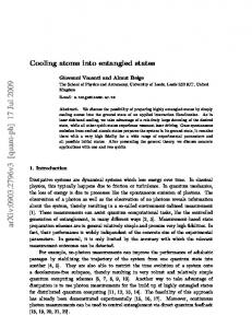
Let us now discuss what are the extremal points of an intersection of two nonempty convex sets S1 and S2 provided that S1 ∩ S2 is nonempty. Recall that a given element x ∈ S is an extremal element of S if it cannot be written as a convex combination of elements from S which are different from x. There are two classes of extremal elements in S1 ∩ S2 – this statement we can formalize as the following (for an illustrative example see Fig. 2).
3 C'
D'
face D
F
C
A'
E
edge vertex A
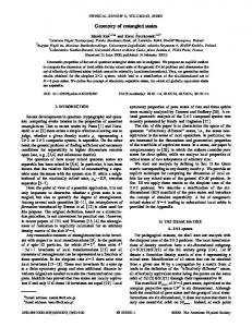
FIG. 1: The dodecahedron on the left and the known cube on the right. A polyhedron consists of polygonal faces, their sides are known as edges, and the corners as vertices. Edges and vertices are also examples of faces of polyhedron.
Observation. Let S1 and S2 be two convex sets. Then the set of extremal points of S1 ∩ S2 consists of: (i) the extremal points of S1 and S2 belonging to S1 ∩ S2 , (ii) possible new extremal points of S1 ∩ S2 which belong to the intersection of boundaries of S1 and S2 and are not extremal points of S1 and S2 . To proceed in a more detailed way let us introduce some definitions. Let S be some convex set and let x, y (x 6= y) be two elements from S. Then any subset of S of the form [x, y] = {λx + (1 − λ)y | x, y ∈ S, 0 ≤ λ ≤ 1} is called closed line segment between x and y. Further, let F be some subset of the convex set S. Then F is called face of S if it is convex and the following implication holds: if for any line segment [x, y] ⊆ S such that its interior point belongs to F then [x, y] ⊆ F . Equivalently, F ⊆ S is a face of S if from the fact x, y ∈ S and (x + y)/2 ∈ F it follows that x, y ∈ F . Thus, x ∈ S is an extremal point of S if the one–element set {x} is a face of S. This definition formalizes the notion of a face of a convex polygon or a convex polytope and generalizes it to an arbitrary convex set. In this sense, vertices of a polytope are zero–dimensional faces (extremal points), edges are one–dimensional faces and the traditionally understood faces are two–dimensional. The interior points form a two–dimensional face (see Fig. 1). On the other hand, any point on the boundary of a closed unit ball in Rn , i.e., any point of the unit (n − 1)–dimensional sphere, is a face (and an extreme point) of the ball. Let us now discuss what are the main conclusions following the above observation. Namely, if some convex sets S1 and S2 intersect in a point x along an affine manifold of non–zero dimension then x cannot be extremal. Therefore x belongs to the second class of extremal points in S1 ∩ S2 if and only if the intersection of the relevant faces is exactly x, i.e., the faces are transversal at x (see Fig. 2). Let us also point out how the above observation can be utilized to prove that a given x is not an extremal element of S1 ∩ S2 . Namely, if x belongs to the intersection of some faces of S1 and S2 , we can consider other element x±ǫy with ǫ denoting some arbitrarily small positive real
B'
B
FIG. 2: A simple example visualizing the observation formulated in Sec. II B. The se of extremal points of the rectangle A′ ECF resulting from an intersection of rectangles ABCD and A′ B ′ C ′ D′ consist of some of the extremal points of both rectangles or the ones that appear as intersections of their respective edges. More precisely, the points A′ and C are extremal points of the rectangles A′ B ′ C ′ D and ABCD, respectively. The Points E and F result from intersection of the edges of these rectangles, namely, A′ B ′ and BC, and CD and D′ A′ , respectively. Both the intersections give manifolds consisting of a single point (the respective edges are transversal).
number and y is an element of the affine space in which S1 and S2 are convex subsets. If such element belongs to the intersection of the mentioned faces the intersection has a non–zero dimension and x cannot be an extremal element of S1 ∩S2 . The key point of this remark is that to generate this manifold we do not have to consider elements of the convex subsets S1 and S2 . This, as we will see in the next subsection, can be applied to convex sets of density matrices with positive partial transposition.
C. Criterion for extremality in convex sets of quantum states with positive partial transposition
In the context of DdPPT the observation of Sec. II B 1 ,d2 says that the set of its extremal points is the sum of two disjoint subsets. The first one consists of pure extremal states of Dd1 ,d2 which are simultaneously extremal points of DdΓ1 ,d2 . The second subset consists of the extremal points that could appear from intersection of boundaries of Dd1 ,d2 and DdΓ1 ,d2 and are not extremal points of both these sets. If a given ̺ is neither an extremal point of Dd1 ,d2 nor of DdΓ1 ,d2 then we have to check (assuming obviously that it is an edge state) if the faces to which ̺ and ̺ΓA belong are transversal. It can be seen that this reduces to the problem of solving a system of linear equations. For this purpose we utilize the technique mentioned in the preceding section of adding or subtracting small elements not necessarily belonging to Dd1 ,d2 or DdΓ1 ,d2 . As we will see below for this aim we can use Hermitian matrices H such that R(H) ⊆ R(̺) and R(H ΓA ) ⊆ R(̺ΓA ). To proceed more formally let us notice that, as we know from Ref. [25], the face of Dd1 ,d2 at
4 a given ̺ (which is not of full rank as only such density matrices constitute faces of Dd1 ,d2 ) consists of matrices of dimensions d1 d2 × d1 d2 with kernels coinciding with the kernel of ̺ (this holds also for partial transpositions of density matrices provided they are positive). On the other hand, all Hermitian matrices of rank k constitute k 2 dimensional subspace of the (d1 d2 )2 –dimensional Hilbert space V (equipped with e.g. the Hilbert–Schmidt scalar product) of all d1 d2 × d1 d2 Hermitian matrices. To check if the intersection V1 ∩ V2 of two subspaces V1 and V2 of dimension k 2 and l2 is nonempty, one has to solve the system of 2(d1 d2 )2 − k 2 − l2 linear equations for (d1 d2 )2 variables. A nontrivial, nonzero-dimensional, solutions exist always if (d1 d2 )2 < k 2 + l2 (in the case of density matrices, due to the normalization, we add one to the left–hand side of this inequality). If our density matrix ̺ has a bi–rank (k, l) admitting the existence of such solutions, it cannot be extremal in DdPPT – one can always 1 ,d2 find a Hermitian matrix H ∈ V1 ∩ V2 with R(H) ⊆ R(̺) and R(H ΓA ) ⊆ R(̺TA ) such that ̺e(ǫ) = ̺±ǫH is positive and PPT. What is important, for small enough ǫ > 0 the matrix ̺e(ǫ) has the same bi–rank as the initial state ̺. From the fact that the face of Dd1 ,d2 at a given ̺ (which is not of full rank as only such density matrices constitute faces of Dd1 ,d2 ) consists of matrices of dimensions d1 d2 × d1 d2 with kernels coinciding with the kernel of ̺ it follows that ̺e(ǫ) has to belong to the same intersection as ̺ and in such case ̺ cannot be extremal in DdPPT . In 1 ,d2 this way we finally arrive at the criterion. Criterion. Let ̺ ∈ Dd1 ,d2 be PPTES with the bi–rank (k, l). If there exists a non-trivial, i.e. non-proportional to ̺, solution of the system of linear equations described above, i.e. equations determining Hermitian matrices H with R(H) ⊆ R(̺) and R(H ΓA ) ⊆ R(̺TA )), then ̺ is not extremal in DdPPT . 1 ,d2 It should be emphasized that the above technique of adding and subtracting Hermitian matrices and the criterion following it were already provided in Ref. [18]. In conclusion, to prove that some ̺ is not extremal in the set of PPT states one can always try to “generate” the nonzero-dimensional manifold by adding or subtracting ǫH with H being a general Hermitian matrix H and ǫ some sufficiently small positive number. This, however, has to be done in such a way that the resulting state ̺e(ǫ) = ̺±ǫH, as well as its partial transposition have the same kernels as, respectively, ̺ and ̺ΓA . More precisely we need to have R(H) ⊆ R(̺) and R(H ΓA ) ⊆ R(̺ΓA )). In this way we remain on the same faces of Dd1 ,d2 and DdΓ1 ,d2 (as the partial transposition of PPT state is still a legitimate state then the observation above works also for partial transpositions of density matrices) as ̺ itself.
III. THE SET OF 2 ⊗ 4 STATES WITH THE POSITIVE PARTIAL TRANSPOSITION
Here, we sketch shortly the overall picture of qubit– ququart states with respect to the extremality in the set
of PPT states. First we recall literature results from which it follows that the only possible cases of PPT entangled states that could be extremal are the ones with bi–rank (5, 5) and (5, 6) (and equivalently (6, 5)), and (6, 6). Next, basing on the observation from Sec. II, we will exclude the case of bi–rank (6, 6). Then, we show PPT that any edge state of bi–rank (5, 5) is extremal in D2,4 which implies that the famous examples of 2 ⊗ 4 PPT entangled states provided in Ref. [5] are extremal. Finally, we present a two–parameter class of edge states that depending on the parameters have bi–rank (5, 6) or (5, 5), giving at the same time next example of extremal (5, 5) states.
A.
The general situation
Let us here discuss shortly why the only possible cases in which there could be PPT entangled extremal states are these of the bi–rank (5, 5), (5, 6) (equivalently (6, 5)), and (6, 6). At the very beginning we can rule out the cases in which either ̺ or ̺ΓA are of full rank since then the density matrix lie in the interior of the set of PPT states (see e.g. Ref. [25]). To deal with the remaining cases we can assume that the given ̺ is supported on full C2 ⊗ C4 . Otherwise we would deal with a state that is effectively qubit–qutrit state and one knows that in this case there are no PPT entangled states [4]. On the same footing we can assume that there is no separable vector |e, f i in the kernel of ̺. Otherwise, it would mean, according to Ref. [12], that ̺ could be written as a mixture of a projector onto the separable vector |e⊥ , hi (with he⊥ |ei = 0, and a certain |hi) and some PPT state supported on C2 ⊗ C3 , and thus separable. In conclusion, in such a case ̺ could be written as a mixture of separable states and thus would be separable itself. We know from Ref. [12] that if ̺ is supported on C2 ⊗ N C and is entangled then r(̺) > N . This means that in what follows we can assume that r(̺), r(̺ΓA ) > 4 as otherwise we would deal with a separable state. Then, following Ref. [12], we divide our considerations into two cases, (i) r(̺) + r(̺ΓA ) ≤ 12, (ii) r(̺) + r(̺ΓA ) > 12. In the second case it was shown in Ref. [12] that there always exists a separable vector |e, f i in the range of ̺ for which |e∗ , f i ∈ R(̺ΓA ). Consequently, we may subtract this vector from ̺ obtaining another (unnormalized) state ̺e = ̺ − η|e, f ihe, f |,
(2)
where η = min{η0 , η 0 } with η0 and η 0 given by η0 = (he, f |̺−1 |e, f i)−1 and η 0 = (he∗ , f |(̺ΓA )−1 |e∗ , f i)−1 . Here ̺−1 denotes the so–called pseudoinverse of ̺, i.e.,
5 inverse of ̺ only on the projectors corresponding to its nonzero eigenvalues. Normalizing ̺e we infer from Eq. (2) that ̺ can be written as ̺ = (1 − η)e ̺ + η|e, f ihe, f |,
(3)
with 0 < η < 1 (this is because both parameters η0 and η 0 satisfy 0 < η0 , η 0 < 1). The important fact here is that the above procedure of subtraction product vectors preserves positivity of partial transposition of ̺. More precisely, if ̺ΓA ≥ then also ̺e ΓA ≥ 0. All these mean that if r(̺) + r(̺ΓA ) > 12 we are always able to write ̺ as a convex combination of two states with positive partial transposition. Thus in this case there are no PPT PPT entangled extremal states in the convex set D2,4 (we see that even edge states do not exist in these cases). So far we have ruled out most of the cases with respect to the bi–rank. What remains are the states satisfying r(̺) > 4, r(̺ΓA ) > 4, and r(̺) + r(̺ΓA ) ≤ 12. In the cases of (5, 7) and (7, 5) it was shown in Ref. [26] that there exists a product vector |e, f i ∈ R(̺) such that |e∗ , f i ∈ R(̺ΓA ). This, according to what was said above, means that also among states with bi–rank (5, 7) or (7, 5) one cannot find PPT entangled extremal states. The case of bi–rank (6, 6) can be ruled out by the criterion. Here k = l = 6 and therefore one has a system of 56 linear homogenous equations for 63 variables (one is subtracted due to normalization). According to what was said in Sec. II C this means that all (6, 6) PPTES are not extremal as for any such state there exist a Hermitian H satisfying R(H) ⊆ R(̺) and R(H ΓA ) ⊆ R(̺ΓA ). Thus an intersection of the corresponding faces of D2,4 Γ and D2,4 is thus a nonzero-dimensional manifold. B.
PPT tremal in D2,4 . This means that it admits the form PPT σ = λσ1 + (1 − λ)σ2 with some λ ∈ (0, 1) and σi ∈ D2,4 (i = 1, 2). Since σ is edge state it is clear that both the density matrices σi have to be entangled. Also, it is easy to see that the conditions R(σi ) ⊆ R(σ) and R(σiΓA ) ⊆ R(σ ΓA ) hold for i = 1, 2. As a conclusion one of these density matrices, say σ1 , can be subtracted from σ with some small portion ǫ > 0 in such a way that the resulting matrix, as well as its partial transposition, remain positive. More precisely, we can consider the state σ e = (σ − ǫσ1 )/(1 − ǫ) which obviously has the rank r(e σ ) ≤ 5. The parameter ǫ can be set so that either r(e σ ) = 4 or r(e σ Γ ) = 4. Consequently, by virtue of results of Ref. [12] where it was shown that any PPT state supported on 2 ⊗ 4 with rank 4 is separable, the latter means that σ e is separable. As a result the initial state σ can be written in the form
σ = (1 − ǫ)e σ + ǫσ1 ,
(5)
which means that σ is a convex combination of a separable and an entangled state. This, however, is in contradiction with the assumption that σ in an edge state. Thus σ has to be extremal what finishes the proof. Notice that the above statement remains true if one relaxes the condition of being an edge state to being a PPT entangled state. That is, all PPT entangled states of bi-rank (5, 5) are extremal. It was shown in Ref. [5] that σ(b) for b ∈ (0, 1) are edge states and therefore, due to the above theorem, they are extremal in the set of 2 ⊗ 4 PPT states. Let us remark that all the cases satisfying r(̺) + r(̺ΓA ) ≥ 12, as well as the case of the bi-rank (5, 7) (and equivalently (7, 5)) can be also ruled out using the criterion.
The case of bi–rank (5, 5)
The remaining cases in which we can look for the extremal PPT states are (5, 5) and (5, 6). In the first case of the bi–rank (5, 5) examples of extremal PPT entangled states can be provided. For instance, we can show that the states found in Ref. [5], b 0 0 0 0 b 0 0 0 0 b 0 0 b 0 0 0 0 0 b 0 0 b 0 0 0 0 √0 1 0 0 0 b σ(b) = , 1 1 2 1 + 7b 0 0 0 0 2 (1 + b) 0 0 2 1 − b b 0 0 0 0 b 0 0 0 b 0 0 0 0 b 0 √ 1 1 2 0 0 b 0 2 1 − b 0 0 2 (1 + b) (4) are extremal for b ∈ (0, 1) (for b = 0, 1 the state is separable). For this aim let us prove the following theorem. Theorem. Any 2 ⊗ 4 edge state with bi–rank (5, 5) is PPT extremal in the set of PPT states D2,4 . Proof. (a.a.) Let us consider an 2 ⊗ 4 edge state σ with the bi–rank (5, 5) and assume that it is not ex-
C.
The case of bi–rank (5, 6)
The last case we need to deal with is the one with the bi–rank (5, 6). It was numerically confirmed in Ref. PPT [18] that there exist (5, 6) extremal PPT states in D2,4 , however, explicit examples are still missing. In what follows let us consider the family of 2 ⊗ 4 PPT entangled states with r(̺) = 5 and r(̺ΓA ) = 6 which are ΓA edge but not extremal in the set D2,4 . The family is of the form ̺(a, t) =
1 2(2 + a + a−1 ) a 0 0 0 1 0 0 0 a−1 0 0 0 × 0 0 0 −1 0 0 0 −1 0 0 0 −1
0 0 0 1 t 0 0 0
0 −1 0 0 0 0 −1 0 0 0 0 −1 t 0 0 0 .(6) 1 0 0 0 −1 0 a 0 0 0 0 1 0 0 0 0 a
6 The vector of eigenvalues of ̺(a, t) reads λ(̺(a, t)) =
1 2(1 + a)2
� × 2a, 1 + a2 , 1 + a2 , a(1 − t), a(1 + t), 0, 0, 0 . (7)
Thus, for a > 0 and −1 < t < 1 the rank of ̺(a, t) is exactly five. Let us now look at the partial transposition of ̺, which is given by [̺(a, t)]ΓA =
1 2(2 + a + a−1 ) a 0 0 0 0 0 0 t 0 1 0 0 −1 0 0 0 0 0 a−1 0 0 −1 0 0 0 1 0 0 −1 0 0 0 . × 0 1 0 0 0 0 −1 0 0 0 −1 0 0 a−1 0 0 0 0 0 −1 0 0 1 0 t 0 0 0 0 0 0 a (8)
The vector of eigenvalues of ̺ΓA is of the form 1 2(1 + a)2 × (1 − a, 2a, 2a, 1, a(a − t), a(a + t), 0, 0) .
λ(̺(a, t)ΓA ) =
(9)
For a ≥ t, a + t ≥ 0, and a < 1 one has [̺(a, t)]ΓA ≥ 0, hnece ̺(a, t) is a PPT state of the bi–rank (5, 6) whenever 0 < a < 1 and |t| < a. For t = a it has the bi–rank (5, 5) and is an edge state (one can check it using the method presented in Ref. [5]). Due to the theorem from Sec. III A PPT it is also another example of an extremal state in D2,4 . To prove that the ̺(a, t) is entangled and thus bound entangled we may use the already mentioned range criterion of Ref. [5]. After some algebra one finds that all the product vectors in the range of ̺(a, t) can be written in the form A(α, t)(1; α) ⊗ (α3 ; −α2 /a; α/a; 1)
(α ∈ C ∪ {∞}), (10) with A being some function of α and t. We used here the fact that any vector from C2 can be written as |0i + α|1i with α ∈ C ∪ {∞} end employed the convention a|0i + b|1i ≡ (a; b) together with a similar one for vectors in C4 . A similar analysis shows that the product vectors in the range of ̺ΓA are of the form (1; α) ⊗ (B(α, a, t), −αB(α, a, t), C(α, a, t), −αC(α, a, t)) (α ∈ C ∪ {∞}), (11) with B and C denoting some functions. Simple calculations show that one cannot find such a product vector |e, f i from R(̺(a, t)) that |e∗ , f i ∈ R(̺(a, t)ΓA ). More precisely, one cannot find such functions B and C in Eq. (11) that the vector A(α, t)(1; α∗ ) ⊗ (α3 ; −α2 /a; α/a; 1) can be written in the above form. Thus, for any a and t satisfying 0 < a < 1 and |t| < a, the matrix ̺(a, t) is a
PPT entangled state. Moreover, the same argument tell us that it is also an edge state. Now, one immediately finds that ̺(a, t) cannot be extremal in the set of 2 ⊗ 4 PPT states. This is because for a fixed a ∈ (0, 1), t ∈ (−a, a) can always be expressed as t = (1 − λ)t1 + λt2 with λ ∈ (0, 1) and ti ∈ (−a, a) (i = 1, 2), which means that for any a ∈ (0, 1) the state ̺(a, t) can be written as the following convex combination ̺(a, t) = (1 − λ)̺(a, t1 ) + λ̺(a, t2 ). IV.
(12)
EXPLORING PPT STATES OF BI–RANK (5, 6)
We continue our considerations in the case of bi–rank (5, 6), however, in the most general situation. As the discussion presented in this section is a bit more mathematically demanding it is helpful to outline first its contents before going into details. The general aim of this section is to explore PPT states with bi–rank (5, 6). It is stated in Ref. [18] that there exist extremal PPTES of this type, however, the general structure of this class of states is not known and the main purpose is to make a first attempt to understand it. For this purpose, using the so–called canonical form of 2⊗N states, we determine all the product vectors in ranges of ̺ and ̺ΓA . Then, using the latter and following the criterion, we propose for any (5, 6) PPT state such a Hermitian matrix H that R(H) ⊆ R(̺) and look if R(H ΓA ) ⊆ R(̺ΓA ). This brings the problem of extremality to the problem of solving a set of linear equations. Although we cannot provide a solution to this system in the general case, we can provide various sets of conditions for B (see Eq. (15)) provided that the solution has some particular form (and the corresponding state is not extremal).
A.
Separable vectors in ranges of ̺ and ̺ΓA in the case of (5, 6)
Let us consider an arbitrary 2 ⊗ 4 state. It can be brought to the so–called canonical form (see e.g. Ref. [26, 27] and Ref. [28] in the context of 2 ⊗ 2 ⊗ N states). To see it explicitly let us notice that any such state has the form � � A B ̺= , (13) B† C where A, B, and C are some 4 × 4 matrices and due to the positivity of ̺ one knows that A and C have to be positive as well. Since we assume that r(̺) = 5, we can also assume that the matrix C is of full rank. Otherwise, one sees to see that the vector |1, f i, where |f i ∈ K(C), belongs to the kernel of ̺. In view of what was said before this means of course that ̺ would be separable.
7 Thus, assuming that r(C) = 4 we can bring ̺ to its canonical form by applying the transformation ̺ 7→ (12 ⊗ C −1/2 )̺(12 ⊗ C −1/2 ), which finally gives � ′ � A B′ ′ ̺ = , (14) B ′† 14 where by 1d we denoted d × d identity matrix. It should be emphasized that the above transformation does not change the rank, extremality as well as separability properties of a given ̺. Thus from our point of view both states ̺ and (12 ⊗ C −1/2 )̺(12 ⊗ C −1/2 ) are completely equivalent. We can simplify the form (14) even further. The positivity of ρ′ implies A′ = B ′ B ′† + Λ, where Λ is some positive matrix. Consequently, omitting all the primes we can write � � BB † + Λ B (15) ̺= 14 , B† where B is some (in general non–Hermitian) matrix. Furthermore, we can assume that det(B) = 0, which means that r(B) = 3 and det(B † ) = 3 and therefore there exist e from C4 that B|φi = 0 and B † |φi e = 0, such |φi and |φi respectively. This can be done by changing the basis in the first subsystem. Precisely, we can apply the transformation U (γ, δ) ⊗ 14 with U (γ, δ) given by � � γ δ , (γ, δ ∈ C \ {0}), (16) U (γ, δ) = −δ ∗ γ ∗ e =0 to ̺. Then it suffices to solve the equation det(B) which always has solutions. Finally, Λ is some positive matrix of rank one and thus can be written as Λ = λ1 |λ1 ihλ1 |. Performing the partial transposition with respect to the first subsystem we get � � � � e B† BB † + Λ B † B†B + Λ ΓA = ̺ , (17) B 14 = 14 B
e = [B, B † ] + Λ = λ2 |λ2 ihλ2 | + λ3 |λ3 ihλ3 |. This with Λ form is similar to the one of ̺ with the difference that e is a combination of two projectors as we want to have Λ r(̺ΓA ) = 6. Let us now find the general form of separable vectors in the ranges ̺ and ̺ΓA and discuss their properties. Due to the similarity of the forms of ̺ and ̺ΓA (see Eqs. (15) and (17)), it suffices to make the calculations for the range of ̺. As any (unnormalized) vector from C2 ⊗ C4 can be always written as |0, gi + |1, hi, this can be done by solving the system of equations ̺(|0, gi + |1, hi) = |ei|f i with |ei ∈ C2 and |gi, |hi, and |f i denoting some vectors from C4 . As previously we can utilize the fact that any vector |ei from C2 can always be written as |ei ≡ |e(α)i = |0i + α|1i with α ∈ C ∪ {∞} (for the sake of simplicity we forget about normalization, however we keep in mind
that |e(0)i = |0i and |e(∞)i = |1i). The resulting set of equations reads ( (BB † + Λ)|gi + B|hi = |f i, (18) B † |gi + |hi = α|f i. After some algebra one finds that the solution is of the form |f i ≡ a|f (α)i = a(14 − αB)−1 |λ1 i,
(19)
with a = λ1 hλ1 |gi). Except for the solutions of det(14 − αB) = 0, the inverse of 14 − αB exists for all α ∈ C. The same reasoning in the case of ̺ΓA gives |fe(α, b, c)i = (1 − αB † )−1 (b|λ2 i + c|λ3 i).
(20)
with appropriate constants b and c. Therefore the separable vectors from R(̺) and R(̺TA ) are of the form a|e(α)i|f (α)i and |e(α)i|fe(α, b, c)i, respectively. With some additional effort we can determine a more detailed form of the separable vectors in the range of ̺ proving that the general form of |f (α)i is |f (α)i =
1 (W1 (α); W2 (α); W3 (α); W4 (α)), W (α)
(21)
with W (α) and Wi (α) (i = 1, . . . , 4) being some polynomials in α of degree at most three. To see this explicitly we notice that since r(̺) = 5 there exist three linearly independent vectors |φi i in K(̺) orthogonal to |e(α)i|f (α)i. Writing them in the form (1) (0) |φi i = |0i|φei i + |1i|φei i,
(22)
we get from the orthogonality conditions (1) (0) hφei |f (α)i + αhφei |f (α)i = 0,
(i = 1, 2, 3).
(23)
P4 By decomposing |f (α)i = k=1 fk (α)|ak i in some basis {|ak i} we get the following system of three homogenous equations � � X (1) (0) (24) fk (α) hφe |ak i + αhφe |ak i = 0. i
i
k
We can always fix the value of one of fk , e.g. by putting f4 (α) = 1, and obtaining 3 X
k=1
� � (0) (1) (0) fk (α) hφei |ak i + αhφei |ak i = −hφei |a4 i (1)
−αhφei |a4 i, (25)
for i = 1, 2, 3. Now we deal with a system of three inhomogenous equations (the inhomogeneity is nonzero as one can always find such basis in C4 that at least one of the scalar products on the right–hand side of
8 (25) is nonzero). Solving the system we get the postulated form (21). Using a little bit more sophisticated reasoning one may also prove that the polynomials Wi (i = 1, 2, 3, 4) are linearly independent and therefore at least one of them must be of the third degree. This also means that all the separable vectors in R(̺) can be brought to the form (1; α) ⊗ (1; α, α2 ; α3 ). Indeed, since Wi (i = 1, 2, 3, 4) are linearly independent there exist matrix V with det(V ) 6= 0 such that 12 ⊗ V ̺12 ⊗ V † has all the separable vectors in its range of the above form. B.
Density matrices of bi–rank (5, 6) that are not extremal
Knowing the general form of product vectors from R(̺) and R(̺ΓA ) of a general qubit–ququart state we can now provide some conditions under which the (5, 6) PPT states are not extremal. For this purpose let us consider the following Hermitian operator H = a1 a2 |e(α1 )ihe(α2 )| ⊗ |f (α1 )ihf (α2 )| + h.c.
(26)
with α1 6= α2 . Its partial transposition with respect to the first subsystem reads H ΓA = a1 a2 |e(α∗2 )ihe(α∗1 )| ⊗ |f (α1 )ihf (α2 )| + h.c. (27) One sees that R(H) ⊆ R(̺), still, however, we need to check if R(H ΓA ) ⊆ R(̺ΓA ). The assumption α1 6= α2 is important since for α1 = α2 one could subtract a product vector from ̺ without spoiling its relevant properties, hence ̺ would not be an edge state. We need to find such α1 , a1 , α2 , and a2 that a1 |e(α2 )i|f (α1 )i = |e(α2 )i|fe(α∗2 , a1 , b1 )i and a2 |e(α∗1 )i|f (α2 )i = |e(α∗1 )i|fe(α∗1 , b2 , c2 )i as both these vectors belong to the range of ̺ΓA . These conditions simplify to a1 |f (α1 )i = |fe(α∗2 , b1 , c1 )i and a2 |f (α2 )i = |fe(α∗1 , b2 , c2 )i, respectively which, in turn, can be brought to a system of linear equations (I − α1 B)|xi = a1 |λ1 i,
(28)
(I − α∗2 B)|xi = b1 |λ2 i + c1 |λ3 i,
(29)
4
where |xi is a vector from C that has to be determined. We can introduce three vectors |fi i (i = 1, 2, 3) orthogonal to |λ1 i and two vectors |vi i (i = 1, 2) orthogonal to |λ2 i and |λ3 i. Projection of Eqs. (28) and (29) onto the vectors |fi i (i = 1, 2, 3) and |λ1 i leads to the following systems of equations ( hfi |I − α1 B|xi = 0, i = 1, 2, 3, (30) hλ1 |I − α1 B|xi = a1 , and onto the vectors |vi i (i = 1, 2) and |λ2 i, and |λ3 i to ∗ † i = 1, 2, hvi |I − α2 B |xi = 0, ∗ † hλ2 |I − α2 B |xi = b1 + c1 hλ2 |λ3 i, (31) ∗ † hλ3 |I − α2 B |xi = b1 hλ3 |λ2 i + c1 .
The same procedure applied to the equation a2 |f (α2 )i = |fe(α∗1 , b2 , c2 )i leads to an analogous system of equations ( hfi |I − α2 B|yi = 0, i = 1, 2, 3, (32) hλ1 |I − α2 B|yi = a2 , ∗ † i = 1, 2, hvi |I − α1 B |yi = 0, ∗ † hλ2 |I − α1 B |yi = b2 + c2 hλ2 |λ3 i, hλ3 |I − α∗1 B † |yi = b2 hλ3 |λ2 i + c2 .
(33)
Together, the homogenous equations in (30), (31), (32), and (33) give ten equations for eight unknowns variables xi and yi (i = 1 . . . , 4) being coordinates of |xi and |yi in some basis in C4 . From the remaining inhomogenous equations one could determine ai , bi , and ci (i = 1, 2). The most natural and, in our opinion, easiest way to solve all the homogenous equations is to consider them separately for |xi and |yi. For this aim let us rewrite the homogenous equations of (30) and (31) as ( hfi |I − α1 B|xi = 0, i = 1, 2, 3, (34) ∗ † hvi |I − α2 B |xi = 0, i = 1, 2. They constitute five linear equations for |xi, which implies that two determinants have to vanish; we take them to involve the first three equations, together with one of the remaining two. In effect each determinant has a form of a third order polynomial in α1 and first order in α∗2 . Such a system of two polynomials has several solutions for the pairs (α1 , α2 ) with α1 6= α2 (if there were a solution α1 = α2 , we could subtract the projector on the corresponding product vector from the state ̺ and the partially transposed one from the partially transposed state keeping the positivity of both, which is incompatible with ̺ being an edge state). The remaining equations, hfi |I − α2 B|yi = 0, with i = 1, 2, 3 and hvi |I − α∗1 B † |yi = 0, with i = 1, 2 we obtain by replacing in (34) |xi → |yi, and α1 → α2 . Concluding, there always exist such pairs of α1 and α2 that the set (34) has a nontrivial solution. Now, if the analogous set of equations for the vector |yi has a solution for the particular α1 and α2 solving (34), but interchanged α1 ↔ α2 , then we have a solution to the initial problem. We cannot find the general solution to this problem and due to results of Ref. [18] it is even impossible. Thus, we consider some particular cases with respect to α1 and α2 , and assuming that the solution is of some particular form we derive certain conditions that have to be satisfied by the matrix B (see Eq. (13)). For α1 = ∞ and α2 = 0 the homogenous equations from (30), (31), (32), and (33) reduce to ( hfi |B|xi = 0, i = 1, 2, 3, (35) hvi |xi = 0, i = 1, 2, and
(
hfi |yi = 0, †
hvi |B |yi = 0,
i = 1, 2, 3 i = 1, 2.
(36)
9 From the first set we see that |xi = ξ|λ2 i + η|λ3 i, while from the second one that |yi = µ|λ1 i. So in the case of α1 = ∞ and α2 = 0 we are able to find |xi and |yi, however the matrix B has to satisfy the conditions hfi |B(ξ|λ2 i + η|λ3 i) = 0 with i = 1, 2, 3 and hvi |B † |λ1 i = 0 for i = 1, 2. In the case α1 = 0 and 0 6= α2 6= ∞ we have � hfi |xi = 0, i = 1, 2, 3, (37) ∗ † hvi |I − α2 B |xi = 0, i = 1, 2, and �
hfi |I − α2 B|yi = 0, hvi |yi = 0,
i = 1, 2, 3, i = 1, 2.
(38)
Here, analogously to the previous case, one has |xi = e 2 i + ηe|λ3 i. Inserting the above forms µ e|λ1 i and |yi = ξ|λ of |xi and |yi to Eqs. (37) and (38) we obtain five conditions for the matrix B. More precisely, we have e 2 i+ hvi |I −α∗2 B † |λ1 i = 0 with i = 1, 2 and hfi |I −α2 B(ξ|λ ηe|λ3 i) = 0 for i = 1, 2, 3. Finally in the case of α1 = ∞ and 0 6= α2 6= ∞ the systems of equations reads ( hfi |B|xi = 0, i = 1, 2, 3, (39) ∗ † hvi |I − α2 B |xi = 0, i = 1, 2, and (
hfi |I − α2 B|yi = 0, †
hvi |B |yi = 0,
i = 1, 2, 3, i = 1, 2.
(40)
All the provided equations in each of the above cases are obviously equipped with conditions of vanishing determinants. V.
MULTI–QUBIT PPT EXTREMAL STATES
It seems interesting to extend the criterion to the case of many–qubits states. In what follows we discuss how it can be applied to the general three and symmetric four qubit states with all partial transposes positive (hereafter PPT states). As we will see in both cases we deal with an intersection of three convex sets. Let us then discuss how extremal points appear when three convex sets S1 , S2 , and S3 intersect provided that S1 ∩ S2 ∩ S3 is not an empty set. Following the observation formulated in the previous sections (we can apply it recursively to the pair of sets S1 and S2 , and then to the pair S1 ∩ S2 , and S3 ) one sees that in general the set of extremal points of S1 ∩ S2 ∩ S3 consists of (i) extremal points of one of these three sets, (ii) points that appear as an intersection of faces of two of these three sets (but are elements of the interior of the remaining set) and are not extremal in any of them, (iii) points that appear as an intersection of faces of all the sets.
A.
Three qubits
At the beginning let us notice that separability properties in three-qubit systems were thoroughly studied in Ref. [28]. Then all these states were classified in Ref. [29]. PPT Let now D2,2,2 be the set (obviously convex) of all three–qubit states having all partial transposes positive. It is clear that positivity of all partial transposes is equivalent to positivity of arbitrary two elementary subsystems, say A and B (positivity of the remaining partial transposes ̺ΓC , ̺ΓAC , and ̺ΓBC is then guaranteed via the positivity of the global transpose). Consequently, PPT D2,2,2 is intersection of three convex sets, namely, the set of all three–qubit density matrices denoted by D2,2,2 and ΓA ΓB two sets D2,2,2 and D2,2,2 containing partially transposed three–qubit density matrices with respect to the A and B subsystem, respectively. By k, l, and m we denote ranks of ̺, ̺ΓA , and ̺ΓB , respectively (generically 1 ≤ k, l, m ≤ 8, however, we can exclude the rank one cases as they are already extremal). First, let us recall that it was shown in Ref. [28] that every three–qubit state ̺ with r(̺) ≤ 3 supported on C2 ⊗ C2 ⊗ C2 is fully separable. Thus we can assume that r(̺), r(̺ΓA ), r(̺ΓB ) ≥ 4 as the same arguments can be applied to ̺ΓA and ̺ΓB . Then, it should be noticed that any three-qubit state can be treated as 2 ⊗ 4 state with respect to the partitions A|BC, B|AC, and C|AB. This, due to results of Ref. [12] means that every three-qubit PPT state with rank r(̺) = 4 is separable across all the above cuts. However, an example of a state separable across A|BC, B|AC, and C|AB cuts but nevertheless entangled was provided in Ref. [14] (the bound entanglement constructed from the so–called unextendible product basis), which as we will see later is PPT . Thus in what follows we can put extremal in D2,2,2 k, l, m ≥ 4. Now, we can follow analogous reasoning as in the bipartite case and obtain the inequality k 2 + l2 + m2 > 65, which if satisfied implies existence of such a Hermitian matrix H that ̺e(ǫ) = ̺ ± ǫH is a density matrix for some nonzero ǫ with all partial transposes positive and the same ranks k, l, m (and thus ̺ of such ranks cannot be extremal). Below we consider only such triples that satisfy k ≤ l ≤ m as the remaining ones one obtains by permuting the ranks k, l, m. It follows immediately from this inequality that there do not exist PPT extremal states of the second kind (see the discussion at the beginning of Sec. V). This is because if one of the ranks is maximal the inequality becomes i2 + j 2 > 1 (i, j = k, l, m) and is always satisfied. On the other hand, application of this inequality to the cases when all ranks are not maximal allows to exclude the following cases (4, 4, 6), (4, 4, 7), (4, 5, 5), (4, 5, 6), (4, 5, 7), (4, 6, 6), (4, 6, 7), and (4, 7, 7). As a result the only cases that remain are (4, 4, 4) and (4, 4, 5). In the first case an example of extremal PPTES was given in [14]. To see it explicitly one may prove a similar statement to the theorem from Sec. IV A. Namely,
10 adapting its proof and utilizing the results of Ref. [28] we get the following theorem. Theorem 2. Any three-qubit PPT entangled state supported on C2 ⊗ C2 ⊗ C2 with ranks r(̺) = r(̺ΓA ) = PPT . r(̺ΓB ) = 4 is extremal in D2,2,2 Since, by construction the three-qubit bound entangled state from Ref. [14] is an edge state it has to be extremal PPT in D2,2,2 of type (4, 4, 4). B.
Four qubits in a symmetric state
In the case of four qubits we restrict our discussion only to the states acting on S((C2 )⊗4 ), which is a subspace of (C2 )⊗4 consisting of all pure states symmetric under permutation of any subset of parties (let us call such states symmetric). General N -qubit symmetric states were recently investigated in numerous papers (see e.g. Refs. [30, 31, 32, 33]). One of the motivations to study four-qubit symmetric states comes from a long–standing open question whether there exist such states with positive partial transpose with respect to all subsystems. If it were so there would also exist extremal PPT symmetric states. Notice that such states, however, with higher number of qubits were found very recently in Ref. [33]. In what follows we would like to discuss what are the possible cases with respect to ranks of respective partial transposes for which there could exist entangled PPT extremal symmetric states. Notice relaxing the PPT condition to two–party transposes only as for instance ̺ΓAB ≥ 0 and leaving the possibility that single–particle partial transposes are nonpositive, it is possible to find four–partite bound entangled symmetric state [34] which even allows for maximal violation of Bell inequality [35]. Interestingly, this state was very recently realized experimentally [36]. Let us discuss firstly some of the properties of mixed states acting on S((C2 )⊗4 ). Clearly, it is√spanned by the vectors |0i⊗4 , |1i⊗4 , |W i, |W i, and (1/ 6)(|0011i + |0101i + |1001i + |1010i + |1100i + |0110i), where |W i is the so–called W state |W i = (1/2)(|0001i + |0010i + |0100i + |1000i) and |W i is obtained from |W i by replacing zeros with ones and vice versa. Consequently, all symmetric four–qubit density matrices have ranks at most five. It also follows from the above that there are only two relevant partial transposes defining set of PPT symmetric states. Namely, positivity of partial transpose with respect to a single subsystem (two subsystems) means positivity of partial transposes with respect to all single subsystems A, B, C, D (arbitrary pairs of subsystems AB, AC, etc.). The three–party partial transposes are equivalent to the single–party partial transposes via the global transposition. Hence, as in the case of three– qubits, the set of PPT symmetric states is an intersection of three sets, namely, the set of symmetric density matrices and the sets of partial transpositions of the latter with respect to the A and AB subsystem, respectively. So, there are three relevant parameters, r(̺), r(̺ΓA ), and
r(̺ΓAB ). Using the fact that we deal with the symmetric states we can easily impose bounds on these three ranks. We already know that r(̺) ≤ 5. Then, since S((C2 )⊗4 ) is a subspace of C2 ⊗ C4 (the A subsystem acts on C2 and the remaining BCD subsystems act on C4 ) it holds that r(̺ΓA ) ≤ 8. On the other hand, S((C2 )⊗4 ) is also a subspace of C3 ⊗ C3 (the two–party subsystems AB and CD act on C3 ) and hence r(̺ΓAB ) ≤ 9. Further constraints on the ranks can be imposed by utilizing results of Refs. [12] and [30]. First of all from Ref. [30] we know that any PPT N –qubit (N > 3) state acting on S((C2 )⊗N ) with r(̺) ≤ N is fully separable, i.e., it can be written as ̺=
X i
(i)
(i)
p i ̺A1 ⊗ . . . ⊗ ̺AN .
(41)
This implies immediately that we can restrict our considerations to r(̺) = 5. The same reasoning can be applied to ̺ΓA and consequently r(̺ΓA ) ≥ 5. Finally, we can treat σ = ̺ΓAB as a three–partite PPT state acting on C2 ⊗C2 ⊗C3 (recall that S(C2 ⊗C2 ) is isomorphic to C3 ). It follows from Ref. [28] that if r(̺ΓAB ) ≤ 3 then σ is a three–partite fully separable (see Eq. (41)) and thus, via reasoning from Ref. [30] ̺ is a four–party fully separable state. Therefore we can assume that r(̺ΓAB ) ≥ 4. Let us now pass to the criterion. The Hermitian matrix we look for has to be also symmetric as we need the condition R(H) ⊆ R(̺) to be satisfied. Consequently r(H) ≤ 5 and we have at most 25 parameters to determine. The condition for r(̺ΓA ) and r(̺ΓAB ) under which H exists can be straightforwardly determined as in the previous cases and reads [r(̺ΓA )]2 + [r(̺ΓAB )]2 > 121, where one follows from the normalization condition. It implies that there are no symmetric PPT extremal states with the following triples of ranks (5, 7, 9), (5, 8, 8), (5, 8, 9) (this agrees with the fact that points being interiors points of two sets and not the extremal point of the third one cannot be extremal points of an intersection of these three sets). All this implies that we have the following ranks for which it is possible that symmetric four–qubit PPT entangled and extremal states exist: r(̺) = 5, 5 ≤ r(̺ΓA ) ≤ 7, and 4 ≤ r(̺ΓAB ) ≤ 8. Still, however, by virtue of Refs. [12] and [30] further simplifications can be inferred. For instance we can treat σ = ̺ΓA as a 2 ⊗ 6 density matrix with respect to the cut B|ACD. Now, if σ is supported on C2 ⊗ Cp (3 < p ≤ 6) then if follows from Ref. [12] that the condition r(̺ΓA ) > p has to be satisfied. Notice that for r(̺ΓA ) = p, σ is separable across B|ACD and therefore ̺ is fully separable. To see this explicitly let us notice that ̺ can be writP (i) (i) (i) (i) ten as ̺ = i pi |eB iheB | ⊗ |ψACB ihψACB |ΓA . Then, it suffices to utilize the fact that tracing out the A subsystem we get three-qubit symmetric density matrix which is separable across the B|CD cut. Finally, utilizing similar approach as the one in Ref. [30] one sees that ̺ has to be fully separable. Analogous arguments work also in the case of ̺ΓAB with respect to e.g. C|ABD cut.
11 In view of what was just said it seems then that generically the only possible cases with respect to ranks (r(̺), r(̺ΓA ), r(̺ΓAB )) are (5, 7, 7), and (5, 7, 8). VI.
CONCLUSION
Let us discuss shortly the presented results. Once more we need to stress that in principle due to results of Gurvits [6] and Doherty [7] the problem of separability in lower dimensional Hilbert spaces can be regarded as solved. Still however, it seems that some progress can be achieved in systems like 3 ⊗ 3 or 2 ⊗ 4. Here one knows that except the states that are detected by the transposition map (NPT states) there are also entangled states with positive partial transposition. As we do not have any unique structural criterion that could detect these PPT states, an attempt to learn about the geometry of the set of PPT states in the lower dimensional systems like 2 ⊗ 4 or 3 ⊗ 3 seems interesting. Some progress in this direction in 3 ⊗ 3 systems has recently been obtained in Refs. [15, 16, 17, 20], where new classes of the edge states have been found for all possible configurations of ranks of a density matrix and its partial transposition. What is even more important examples of these states with bi–ranks (4, 4), (5, 5), and (6, 6) were shown to be extremal in the set of PPT states in Refs. [19, 20, 21]. The main purpose of the paper was to study extremality in the convex set of PPT states in qubit–ququart systems and the main purpose was to provide a operational criterion allowing to judge if a given ̺ is extremal. At the proof stage we learned, however, about Ref. [18] (see also Ref. [19]) in which similar criterion has already been given. In this work we have provided our formulation of the criterion. It reduces the question of extremality to the problem of solving a system of linear equations. Using this approach we have reconstructed the known literature results, i.e., that there are no extremal states in PPT ranks of which satisfy r(̺) + r(̺ΓA ) ≥ 12 (except D2,4 for the case of r(̺) = r(̺ΓA ) = 6). We have investigated the remaining cases of the bi–rank (5, 5), (5, 6),
[1] R. Horodecki, M. Horodecki, P. Horodecki, and K. Horodecki, Rev. Mod. Phys. 81, 865 (2009). [2] A. Peres, Phys. Rev. Lett. 77, 1413 (1996). [3] M.–D. Choi, Positive linear maps, in: Operator Algebras and Applications, Kingston, 1980, Proc. Sympos. Pure Math., vol. 38. Part 2, Amer. Math. Soc., 1982, pp. 583590. [4] M. Horodecki, P. Horodecki, and R. Horodecki, Phys. Lett. A 223, 1 (1996). [5] P. Horodecki, Phys. Lett. A 232, 333 (1997). [6] L. Gurvits, arXiv:quant-ph/0201022; STOC 69, 448 (2003). [7] Doherty, A. C., P. A. Parrilo, and F. M. Spedalieri, Phys. Rev. Lett. 88, 187904 (2002); Phys. Rev. A 69, 022308
and (6, 6). In the case of (6, 6) the criterion shows that there are no extremal states. In the case of bi–rank (5, 5) we proved that all the (5, 5) edge states are extremal in PPT D2,4 implying that the famous Horodecki PPT states [5] are extremal. On the other hand, existence of PPT entangled extremal states of bi–rank (5, 6) has been confirmed numerically in Ref. [18], however, without giving explicit examples. It means that in the 2⊗4 systems only the PPT entangled states of bi–rank (5, 5) and (5, 6) can be extremal. We have also provided a class of states that for some parameter region are (5, 6) edge states, while for some other parameter region they constitute other examples of (5, 5) extremal states. Using the criterion, we have made an attempt to study the structure of (5, 6) PPT states. For any (5, 6) ̺ we provided such a Hermitian H that R(H) ⊆ R(̺), while the condition R(H ΓA ) ⊆ R(̺ΓA ) holds if some corresponding set of linear equations has a solution. We asked what are the conditions imposed on the matrix B (see Eq. (13)) if the solutions are of some particular form. It is shown that whenever B satisfies the corresponding conditions the solution to the system of equations exists. Finally, we extended our considerations on extremality to the simple systems of many-qubits as general threequbit and four-qubit symmetric PPT states. In the first case we have shown that the only cases with respect to the respective ranks in which one may expect extremal PPTES are (4, 4, 4) and (4, 4, 5).
Acknowledgments
We are grateful to J. M. Leinaas for bringing our attention to Ref. [18]. R. A. acknowledges discussion with J. Stasi´ nska. We acknowledge Spanish MEC/MINCIN projects TOQATA (FIS2008-00784) and QOIT (Consolider Ingenio 2010), ESF/MEC project FERMIX (FIS2007-29996-E), EU Integrated Project SCALA, EU STREP project NAMEQUAM, ERC Advanced Grant QUAGATUA, and Alexander von Humboldt Foundation Senior Research Prize.
(2004); ibid. 71, 032333 (2005). [8] C. Su and K. W´ odkiewicz, Phys. Rev. A 44, 6097 (1991); K. W´ odkiewicz, in Foundation of Quantum Mechanics, edited by T. D. Black et al. (World Scientific Publishing, Singapore, 1992); Int. J. Theor. Phys. 31, 515 (1992); Acta Phys. Pol. A 86, 223 (1994); Phys. Rev. A 52, 3503 (1995); B.–G. Englert and K. W´ odkiewicz, Phys. Rev. A 65, 054303 (2002); M. Stobi´ nska and K. W´ odkiewicz, Phys. Rev. A 71, 032304 (2005); Int. J. Mod. Phys. B 20, 1504 (2006); B.–G. Englert and K. W´ odkiewicz, Phys. Rev. A 65, 054303 (2002); L. Praxmeyer, B.–G. Englert, and K. W´ odkiewicz, Eur. Phys. J. D 32, 227 (2005); A. Ch¸eci´ nska and K. W´ odkiewicz, Phys. Rev. A 76, 052306 (2007); ibid., in press (arXiv:0809.3882).
12 [9] K. Banaszek and K. W´ odkiewicz, Phys. Rev. A 58, 4345 (1998); Phys. Rev. Lett. 82, 2009 (1999); Acta Phys. Slov. 49, 491 (1999); K. W´ odkiewicz, New J. Phys. 2, 211 (2000); S. Daffer, K. W´ odkiewicz, and J. K. McIver, Phys. Rev. A 68, 012104 (2003); F. Haug, M. Freyberger, and K. W´ odkiewicz, Phys. Lett. A 321, 6 (2004). [10] K. W´ odkiewicz, L. W. Wang, and J. H. Eberly, Phys. Rev. A 47, 3280 (1993); K. Banaszek, A. Dragan, K. W´ odkiewicz, and C. Radzewicz, Phys. Rev. A 66 043803 (2002); L. Praxmeyer and K. W´ odkiewicz, Laser Phys. 15, 1477 (2005); A. Dragan and K. W´ odkiewicz, Phys. Rev. A 71 012322 (2005); K. Rz¸az˙ ewski and K. W´ odkiewicz, Phys. Rev. Lett. 96, 089301 (2006). [11] M. Lewenstein, B. Kraus, J. I. Cirac, and P. Horodecki, Phys. Rev. A 62, 052310 (2000); M. Lewenstein, B. Kraus, P. Horodecki, and J. I. Cirac, Phys. Rev. A 63, 044304 (2001). [12] B. Kraus, J. I. Cirac, S. Karnas, and M. Lewenstein, Phys. Rev. A 61, 062302 (2000). [13] A. Sanpera, D. Bruss, and M. Lewenstein, Phys. Rev. A 63, 050301(R) (2001). [14] C. H. Bennett, D. P. DiVincenzo, T. Mor, P. W. Shor, J. A. Smolin, and B. M. Terhal, Phys. Rev. Lett. 82, 5385 (1999). [15] K.–C. Ha and S.–H. Kye, J. Phys. A: Math. Gen. 38 9039 (2005). [16] C. Lieven, Phys. Lett. A 359, 603 (2006). [17] K.–C. Ha, Phys. Lett. A 361, 515 (2007). [18] J. M. Leinaas, J. Myrheim, and E. Ovrum, Phys. Rev. A 76, 034304 (2007). [19] K.–C. Ha, Phys. Lett. A 373, 2298 (2009). [20] K.–C. Ha, S.–H. Kye, and Y. S. Park, Phys. Lett. A 313, 163 (2003). [21] W. C. Kim and S.–H. Kye, Phys. Lett. A 369, 16 (2007). ˙ [22] I. Bengtson and K. Zyczkowski, Geometry of Quantum
States, (Cambridge Univ. Press, Cambridge 2006). [23] R. F. Werner, Phys. Rev. A 40, 4277 (1989). [24] M. Horodecki, P. Horodecki, and R. Horodecki, Phys. Rev. Lett. 80, 5239 (1998). [25] J. Grabowski, M. Ku´s, and G. Marmo, J. Phys. A 38, 10217 (2005). [26] J. Samsonowicz, M. Ku´s, and M. Lewenstein, Phys. Rev. A 76, 022314 (2007). [27] P. Horodecki, M. Lewenstein, G. Vidal, and I. Cirac, Phys. Rev. A 62, 032310 (2000). [28] S. Karnas and M. Lewenstein, Phys. Rev. A 64, 042313 (2001). [29] A. Ac´ın, D. Bruss, M. Lewenstein, and A. Sanpera, Phys. Rev. Lett. 87, 040401 (2001). [30] K. Eckert, J. Schliemann, D. Bruss, and M. Lewenstein, Ann. Phys. 299, 88 (2002). [31] J. K. Korbicz, J. I. Cirac, and M. Lewenstein, Phys. Rev. Lett. 95, 120502 (2005); Phys. Rev. Lett. 95, 259901 (2005); J. K. Korbicz, O. G¨ uhne, M. Lewenstein, H. H¨ affner, C. F. Roos, and R. Blatt, Phys. Rev. A 74, 052319 (2006). [32] A. R. Usha Devi, R. Prabhu, A. K. Rajagopal, Phys. Rev. Lett. 98, 060501 (2007). [33] O. G¨ uhne and G. T´ oth, Phys. Rev. Lett. 102, 170503 (2009); Separability criteria and entanglement witnesses for symmetric quantum states, arXiv:0908.3679. [34] J. A. Smolin, Phys. Rev. A 63, 032306 (2001). [35] R. Augusiak and P. Horodecki, Phys. Rev. A 74, 010305 (2006). [36] E. Amselem and M. Bourennane, Nat. Phys. 5, 748 (2009). [37] After acceptance of the previous version of the manuscript (see arXiv:0907.4979v2), J. M. Leinaas brought our attention to to Ref. [18].