pattern and, in this example, leads to a changed direction and a new base point. The revised pattern is applied, but the move is a failure, so the next base point ...
Searching for Tight Performance Bounds in Feed-Forward Networks Andreas Kiefer, Nicos Gollan, Jens B. Schmitt Distributed Computer Systems Lab (DISCO), TU Kaiserslautern, Germany
Abstract. Computing tight performance bounds in feed-forward networks under general assumptions about arrival and server models has turned out to be a challenging problem. Recently it was even shown to be NP-hard [1]. We now address this problem in a heuristic fashion, building on a procedure for computing provably tight bounds under simple traffic and server models. We use a decomposition of a complex problem with more general traffic and server models into a set of simpler problems with simple traffic and server models. This set of problems can become prohibitively large, and we therefore resort to heuristic methods such as Monte Carlo. This shows interesting tradeoffs between performance bound quality and computational effort.
1
Motivation and Related Work
When designing or analyzing a network, one of the most important aspects is its performance under various load conditions. A number of methods for that kind of analysis have been devised, among them network calculus, which describes methods for calculating performance bounds, i.e., describing worst-case behavior. Network calculus is a (min, +) system theory for deterministic queuing systems which builds on the calculus for network delay in [2, 3]. The important service curve concept was introduced in [4–8] to perform efficient analysis of tandem queues. Scaling properties in the number of traversed network nodes are linear, as is shown in [9], a phenomenon also known as pay bursts only once phenomenon [10]. Detailed descriptions of the (min, +) algebra and of network calculus can be found in [11] and [10, 12]. Network calculus has found numerous applications, most prominently in the Internet’s Quality of Service (QoS) proposals IntServ and DiffServ [13, 14], but it has also become a valuable method in other fields, such as wireless sensor networks [15, 16], switched Ethernets [17], Systems-on-Chip (SoC) [18], or even to speed-up simulations [19]. However, as a relatively young theory, compared to, e.g., traditional queueing theory, there is also a number of challenges network calculus still has to master. A very tough challenge is found in the treatment of non-tandem topologies with aggregate multiplexing of multiple flows. While this has been addressed from the beginning [3], there are still many open issues. For aggregate multiplexing in general network topologies there is a very fundamental issue about
the circumstances under which a finite delay bound exists at all [20, 21]. In [22] a sufficient condition for stability in general network topologies and an explicit delay bound are given. Extensions of this approach are provided in [23, 24]. Yet, for larger networks this severely limits the utilization of the network since the maximum allowable utilization is inversely proportional to the network diameter. The problems in the analysis of general topologies arise from cyclic dependencies between flows and the resulting difficulties in bounding their network-internal burstiness. A special class of topologies which avoids those problems are feedforward networks, which are known to be stable for all utilizations ≤ 1 [3]. In this paper, we focus on this class of networks. While many networks are obviously not feed-forward, many important instances like switched networks, wireless sensor networks, or MPLS networks with multipoint-to-point label switched paths are, or can be made, feed-forward by using, e.g., the turn-prohibition algorithm [25]. In feed-forward networks, there has been some work on aggregate multiplexing recently: [26] treats the case of feed-forward networks under FIFO multiplexing for token-bucket constrained flows and rate-latency servers, showing that the derived left-over service curve for a flow of interest is again of the rate-latency type with minimally possible latency. [27] shows that this does not result in a tight delay bound, and derives tight delay bounds under knowledge about the arrival curve of the flow of interest for the special case of sink-trees and, again, under token bucket constrained flows and rate-latency servers. Another work [28] also investigates sink-tree networks, but now under dual token-bucket constrained flows and constant rate servers, for which delay bounds are derived by summing per-node bounds, which unsurprisingly does not yield tight bounds but is still reported as being close under practical conditions. Besides being very specific with respect to traffic and server models, all of the above work assumes FIFO aggregate multiplexing. However in practice, as argued in [29], many devices cannot be accurately described by FIFO because packets arriving at the output queue from different input ports may experience different delays when traversing a node. This is due to the fact that many networking devices like routers are implemented using input-output buffered crossbars and/or multistage interconnections between input and output ports. Hence, packet reordering on the aggregate level is a frequent event (unlike on the flow level) and should not be neglected in modelling. Therefore, in this work we drop the FIFO multiplexing assumption and make essentially no assumptions on the way aggregates are multiplexed at servers, i.e. we assume arbitrary multiplexing also known as general or blind multiplexing [2, 10]. On the level of a single flow, however, we still assume FIFO. This assumption is sometimes called FIFO-per-microflow [30] or locally FCFS multiplexing [2]. Work on bounds for networks with arbitrary multiplexing has become frequent only recently, but there are already several important results. Some older results are reported in [10] (see Section 2), and there is some work on the burstiness increase due to arbitrary multiplexing at a single node [31]. Adversarial queueing theory [32] provides results for general networks, however it is more concerned with network stability than with the determination of performance
bounds. In previous work related to network calculus tool support, we have proposed and implemented a number of network calculus analysis methods for arbitrary multiplexing in feed-forward networks [33], but as will be demonstrated here, they were not the ultimate solution. A similar approach has been taken in [34], regarding a wider class of traffic and service specifications. The goal of our work is to search for tight delay bounds in feed-forward networks of arbitrary multiplexers. With respect to traffic and server models we address a more general case than previous work on FIFO multiplexing, in particular we assume piecewise linear concave arrival curves and convex service curves, which encompass the majority of practical traffic and server models. Compared to our previous work in [35], we now try to solve an issue that arises from the algebra used in network calculus, which, while allowing for an easy analysis, hides certain properties, and may lead to pessimistic bounds. After a short introduction to network calculus, we present an approach to network analysis based on an optimization problem, and show how a solution to that problem can be approximated by heuristics. We show how the quality of the performance bounds obtained by that new method compares with traditional results.
2
Network Calculus Background
As network calculus is built around the notion of cumulative functions for input and output flows of data, the set of real-valued, non-negative, and wide-sense increasing functions passing through the origin plays a major role: F = {f : R+ → R+ |∀t ≥ s : f (t) ≥ f (s) , f (0) = 0 } In particular, the input function F (t) and the output function F ′ (t), which cumulatively count the number of bits that are input to, respectively output from, a system S, are in F . Throughout the paper, we assume in- and output functions to be continuous in time and space. Note that this is not a general limitation as there exist transformations between discrete and continuous time models [10]. Definition 1. (Min-plus Convolution and Deconvolution) The min-plus convolution ⊗ and deconvolution ⊘ of two functions f, g ∈ F are defined as (f ⊗ g) (t) = inf {f (t − s) + g(s)} 0≤s≤t
(f ⊘ g) (t) = sup {f (t + u) − g(u)} u≥0
It can be shown that the triple (F , ∧, ⊗), where ∧ denotes the pointwise minimum operator, constitutes a dioid [10]. Also, the min-plus convolution is a linear operator on the dioid (R ∪ {+∞}, ∧, +), whereas the min-plus deconvolution is not. These algebraic characteristics result in a number of rules that apply to those operators, many of which can be found in [10, 12]. Let us now turn to the performance characteristics of flows which can be bounded by network calculus means:
Definition 2. (Backlog and Delay) Assume a flow with input function F that traverses a system S resulting in the output function F ′ . The backlog of the flow at time t is defined as x(t) = F (t) − F ′ (t) Assuming FIFO delivery, the virtual delay for a bit input at time t is defined as d(t) = inf {τ ≥ 0 : F (t) ≤ F ′ (t + τ )} Next, the arrival and departure processes specified by input and output functions are bounded based on the central network calculus concepts of arrival and service curves: Definition 3. (Arrival Curve) Given a flow with input function F a function α ∈ F is an arrival curve for F iff ∀t, s ≥ 0, s ≤ t : F (t) − F (t − s) ≤ α(s) ⇔ F ≤ F ⊗ α A typical example of an arrival curve is given by an affine arrival curve γr,b (t) = b + rt, t > 0 and γr,b (t) = 0, t ≤ 0 which corresponds to token-bucket traffic regulation. Definition 4. (Service Curve) If the service provided by a system S for a given input function F results in an output function F ′ we say that S offers a service curve β iff F′ ≥ F ⊗ β A typical example of a service curve is given by a so-called rate-latency function + + βR,T (t) = R [t − T ] , where [x] := x∨0, and ∨ denotes the maximum operator. A number of systems fulfill, however, a stricter definition of the service curve [10], which is particularly useful as it permits certain derivations that are not feasible under the more general minimum service curve model. Definition 5. (Strict Service Curve) Let β ∈ F . System S offers a strict service curve β to a flow if during any backlogged period of duration u, the output of the flow is at least equal to β(u). Note that any strict service curve is also a service curve, but not the other way around. Many schedulers offer strict service curves, for example most of the generalized processor sharing-emulating schedulers offer a strict service curve of the rate-latency type. Strict service curves will play a crucial role in this paper, since they, in contrast to service curves, allow to bound the maximum backlogged period of a system. More specifically, that bound d¯ is given � � as the non-zero intersection point between arrival and service curve, i.e. α d¯ = β d¯ . Using those concepts it is possible to derive tight performance bounds on backlog, (virtual) delay and output: Theorem 1. (Performance Bounds) Consider a system S that offers a service curve β. Assume a flow F traversing the system has an arrival curve α. Then we obtain the following performance bounds:
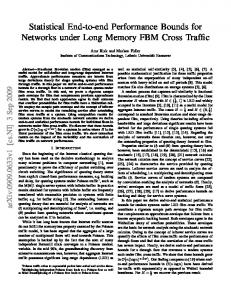
Fig. 1. General network topology. Arrival processes and service characteristics are labeled as described in Section 2. Flows are specified as Fi,j , where i and j denote the ingress and egress nodes. The analysis covers all nodes that the flow of interest Fint passes through.
Backlog: ∀t : x(t) ≤ (α ⊘ β) (0) =: v(α, β) Delay: ∀t : d(t) ≤ inf {t ≥ 0 : (α ⊘ β) (−t) ≤ 0} =: h (α, β) Output (arrival curve α′ for F ′ ): α′ =α ⊘ β One of the strongest results of network calculus (albeit being a simple consequence of the associativity of ⊗) is the concatenation theorem that enables us to investigate tandems of systems as if they were single systems: Theorem 2. (Concatenation Theorem for Tandem Systems) Consider a flow that traverses a tandem of systems S1 and S2 . Assume that Si offers a service curve βi , i = 1, 2 to the flow. Then the concatenation of the two systems offers a service curve β1 ⊗ β2 to the flow. Using the concatenation theorem, it is ensured that an end-to-end analysis of a tandem of servers still achieves tight performance bounds, which in general is not the case for an iterative per-node application of Theorem 1. So far we have only covered the single flow case, the next result factors in the existence of other interfering flows. In particular, it states the minimum service curve available to a flow at a single node under cross-traffic from other flows at that node. Theorem 3. (Left-over Service Curve under Arbitrary Multiplexing) Consider a node multiplexing two flows 1 and 2 in arbitrary order. Assume that the node guarantees a strict minimum service curve β to the aggregate of the two flows. Assume that flow 2 has α2 as an arrival curve. Then β 1 = [β − α2 ]+ is a service curve for flow 1 if β 1 ∈ F , often also called the left-over service curve for the flow of interest. Note that we require the service curve to be strict. In [10], an example is given showing that the theorem otherwise would not hold.
3
Optimization-Based Approach
To analyze a network as shown in Figure 1, conventional methods are the Separated Flow Analysis (SFA) and the Pay Multiplexing Only Once analysis, abbreviated PMOO-SFA since it is an extension of the SFA. A detailed discussion
delay bound [s]
2.0
1.5
analyses PMOO−SFA SFA TIGHT
1.0
0.5
5
10
15
20
25
nodes
Fig. 2. Bound quality comparison. Results are taken from a feed-forward network at 50% utilization. “TIGHT” shows results of the method presented in [36].
Fig. 3. Sample topology that exposes the weakness of the PMOO-SFA. Also shown are (n) the slack variables si,j that are used by the optimization-based approach. The indices i, j denote the ingress and egress servers of a flow, and (n) denotes the hop.
of those methods can be found in [33]. Those methods, as mentioned, offer relatively simple algebraic means to calculate delay bounds for a given feed-forward network, but as shown in [36, 37], those bounds can be made arbitrarily pessimistic by choosing an antagonistic network topology. An example of numerical results comparing different analysis methods is shown in Figure 2. It is obvious that the delay bounds obtained by the SFA are exceedingly pessimistic, while PMOO results at least expose a saner growth behavior. In a similar manner, it can be shown that for some traffic characteristics, the PMOO yields arbitrarily worse results than the SFA, even for very simple topologies like the one shown in Figure 3. We now introduce an approach based on the transformation of the problem to a system of linear programs that was first presented in [36]. The motivation for this new approach becomes obvious when exploring a weakness of the PMOOSFA. While that analysis looks like a perfect application of network calculus principles, it can be shown that applying the convolution to obtain an end-toend service curve for the flow of interest destroys information about the sequence of servers. While the commutativity of the convolution is algebraically nice, it also means that the burstiness of the traffic is always paid for at the rate of the slowest server, even if the structure of the network and the cross-traffic do not require it. While that is not a serious shortcoming in rather homogeneous
networks, it becomes more of an issue in networks where servers are successively faster towards the sink. To work around that shortcoming, we need to find a way to distribute the burst to the servers where it has to be paid, as opposed to the slowest server. To allow for that, slack variables are introduced to represent the accumulated (n) burstiness up to a given server. Those variables are shown as si,j in Figure 3. From those slack variables and with constraints resulting from the traffic and service specifications, it is possible to construct a linear program that finds the left-over service curve for the flow of interest. A thorough discussion of generating the linear programs for a given network, as well as an example can be found in [37]. We will present the core result for analyzing networks with traffic adhering to arrival curves composed from a number of token-buckets, and service curves composed from a number of rate-latency curves, the decomposition theorem, along with a method to use it, as well as numerical results in the following sections.
4
Heuristic Search
When looking at the results so far, we are facing a dilemma: we can either choose to use computationally cheap algorithms at the expense of potentially highly pessimistic bounds, or we can achieve tight bounds at the cost of possibly prohibitively high costs. As is often the case in such a situation, a heuristic approach seems promising, so we propose a new approach to search for tight bounds based on the following decomposition theorem (see [36] for the proof): V W Theorem 4. (Decomposition theorem) Let C and C denote the minimum and maximumVover a set C of curves. Then given piecewise linear concave arrival n curves αi = kii=1 γrki ,bki for each interfering flow i = 1, . . . , n and piecewise W mj linear convex service curves βj = lj =1 βRlj ,Tlj for each node j = 1, . . . , m on the path of the flow of interest, the left-over service curve for the flow of interest is given by mj ni _ n _ m _ _ l.o. β l.o. ≥ β{k (1) i },{li } i=1 j=1 ki =1 lj =1 l.o. are end-to-end left-over service curves for a specific combinawhere β{k i },{lj } tion of a single token bucket per interfering flow and a single rate-latency curve per node.
This leads to a set of linear programs that have to be solved, since each combination of arrival and Qnservice Qm segment generates one. For piecewise linear curves, we get systems of i=1 j=1 ni mj programs. So if we assume for example arrivals adhering to a T-Spec curve (i.e., two segments), and mj -segment service 2m curves for two flows (n = 2) over m servers, we get (2m) j linear programs, so the problem size is polynomial in the number of nodes, but exponential in the
number of segments in the arrival and service curves. This means a large number of linear programs with a discrete search space. Since a complete coverage of such a huge search space would mean an extreme expense of computational resources, we decided on a heuristic approach. 4.1
Monte Carlo Search
For reference, we implemented a pure Monte Carlo search. That method does not make any assumptions about the structure of the search space, and is relatively easy to implement. The search space consists of the token-bucket and rate-latency segments the arrival and service curves are composed of, and one iteration of the Monte Carlo method just picks a random segment of each arrival curve and service curve, and calculates a delay for the resulting left-over service curve. While that approach may lead to some intermediate infinite delay values when the arrival curve segments have a higher rate than the service curve segments, those results will be discarded as soon as a feasible combination is encountered. 4.2
Hooke and Jeeves “Direct Search”
For our heuristic search, we combined the Monte Carlo search with a local search algorithm, the “Direct Search” by Hooke and Jeeves [38] (H-J). This search minimizes a function S (φ) of several arguments φ = (φ1 , . . . , φk ) that can be interpreted as a k-dimensional space. The strategy is to vary the arguments of φ until a minimum of S (φ) is found. Here, we are minimizing the delay bound. The algorithm is separated into two important phases. The first phase is to acquire knowledge of the behaviour of S (φ). Therefore, the neighbourhood of a point is explored to establish a pattern of movement for which it is likely to find a lesser value. Each exploratory move is expected to be simple, that means each move varies only a single argument φi at a time by first increasing and afterwards decreasing it by the current step size ∆. The second phase applies the resulting pattern to the point with the lowest value of S (φ) found up to that point. If that pattern move is successful, i.e., the corresponding functional value is lower, then the new point is the base point for the next exploration. Otherwise, the exploration starts from the point with the minimal functional value so far. The regularly performed exploration revises the pattern continually. If the exploration is a failure, the current step size ∆ is reduced by a reduction factor ρ < 1 until the minimum step size δ is reached. Figure 4 illustrates the process. Starting at an arbitrarily chosen base point, both the increase of the first and second dimension φ1 and φ2 are successful. The acquired pattern is used for the following pattern move to get to the next base point. At each base point, the exploration phase starts again to revise the pattern and, in this example, leads to a changed direction and a new base point. The revised pattern is applied, but the move is a failure, so the next base point is
φ1
exploratory move pattern move pattern
e2 e1
success b failure bc end ⊗
⊗
p1
Start
0
φ2
Fig. 4. Illustration of the moves taken by the Hooke and Jeeves optimization method. Exploratory moves to the top/right are steps of size +∆, and −∆ towards the bottom/left. The first two exploratory moves e1 and e2 establish the pattern p1 which is then used for the first pattern move.
set to the last successful move, and the exploration phase continues from there. The search now stops because no successful move can be made. To apply the H-J algorithm to our workspace, we need to map the arrival and service curves to the k dimensions φi and define how to increase and decrease it by the step size ∆. Each dimension will contain a list composed of segments of individual curves. If, for example, a dimension consists of two arrival curves, α1 with 2 token-bucket components and α2 with 3 token-bucket components, then the dimension is made up from lists [i1 , i2 ] with i1 ∈ {0, 1} and i2 ∈ {0, 1, 2} as the zero-based indices of the token-bucket components of the individual curves. Stepping through such a dimension is implemented through an appropriate enumeration scheme. We analyze the Optimization-Based Approach (OBA) with two mappings of curves to dimensions: – A two-dimensional mapping (OBA-HJTwo), using one dimension to represent all arrival curves, and the other for the services. – A multi-dimensional mapping (OBA-HJMulti) with still only one dimension for the services, but the arrivals are handled as one dimension for each ingress node.
5
Results
For the numerical experiments, our network calculus tool, the DISCO Network Calculator [39, 40] was extended significantly to perform the decomposition and generation of the linear programs. The generated programs were handed off
to lp solve [41], but other linear solvers can also be used by implementing an interface. The implementation involved major refactoring, and we are planning to make that implementation publicly available with an upcoming new release. The hardware used for the calculations was similar to commonly available desktop computers, running on Intel’s Core 2 architecture Xeons. An optimization run with 15 nodes used only up to 1.1GB of RAM. Since the implementations of the DNC and lp solve are single-threaded, a single instance of the problem would run comparably on common off-the-shelf hardware.
5.1
Experimental Design
For our experiments, we used the general network topology as shown in Figure 1. This is a simplified view of the network from the flow of interest’s perspective and implies that all flows that share the same ingress and egress node are seen as only one flow. We assumed a fully occupied network – so for each pair of nodes (i, j) with i ≤ j there was a flow Fi,j – and realistic data flow characteristics for our workload. Hence, to generate arrival curves for the cross-traffic, we have chosen the following setup. At first arbitrary T-SPECs [42] (M, p, r, b) are generated to simulate realistic envelopes. Each T-SPEC is constrained by the following constant parameters burst size b = 1M b, maximum packet size M = 1500bit, and sustained rate r = 1M bps. The peak rate p is arbitrarily chosen amongst 18 fixed values between pmax = 10M bps and pmin = 1.5M bps. For each flow Fi,j , 32 random T-SPECs are added up. Each node offers a strict rate-latency service curve with a latency of 0.1ms and a service rate dimensioned so that a target utilization of 50% is achieved. The flow of interest is constrained by a token-bucket with a burstiness of b = 8M b and a rate of r = 1M bps. In the experiment we compare, under a varying number of server nodes, the SFA as a representative of the traditional methods, and the heuristic methods OBA-MC (Monte Carlo), OBA-HJTwo, and OBA-HJMulti as described in Section 4. For the runtime, there is a tradeoff to be made between the search space and the number of points sampled by the heuristics. Regardless of the maximum number of combinations, MC samples always 5000 points, even in topologies with less than three nodes (in those cases, we achieve a maximum coverage of over 100%). Since the “intelligent” optimization methods can stop early if they get trapped in a local minimum, there would be a disparity if we had strict limits for the number of starting points and the maximum number of steps. We decided to let the H-J methods run for the same number of points as the MC search with a maximum of 50 steps from a given starting point, and repeat this until it did 5000 steps, so those methods sample upwards of 100 starting points. All experiments were repeated 20 times with new randomly generated traffic and service characteristics.
OBA(HJ−Mult) OBA(HJ−Two)
OBA(MC) SFA
10 9 8 7 6 5 4 3 2 1
Coverage: 1 10−20
Delay [s]
10−40 10−60 10−80 10−100 10−120
1
2
3
4
5
6
7
8 9 nodes
10
11
12
13
14
15
Fig. 5. Comparison of delay bound quality stating 95% confidence level. Also shown is the coverage of the search space on a logarithmic scale (decreasing series). From best to worst, the delay bounds are: multi-dimensional H-J, Monte Carlo, 2-dimensional H-J, and SFA.
5.2
Evaluation
The delay bounds for different methods over number of nodes are shown in Figure 5, connecting the mean values for visual reference. Overall, the results of the heuristic methods look very promising, and expose similar growth properties for the delay bound as the delay bounds obtained by complete coverage in Figure 2, even though they only cover a small part of the search space. When comparing the results of the Direct Search methods with the pure Monte Carlo search, we see two trends: It can be said with 95% confidence, that from 12 nodes on, the HJMulti method does significantly better than Monte Carlo. For 8 to 11 nodes the mean differs, but we cannot make a clear statement with 95% confidence. The figure also shows, that there is a difference between H-J with two and multiple dimensions, which is significant with 95% confidence for 4 nodes and up. However, the two-dimensional direct search has a tendency to yield worse results than Monte Carlo. This can be explained by taking a look at the different structure or the search spaces. Because in our setting, each service curve has only one rate-latency component, that dimension will not change during exploration. Grouping all arrival curves in only one dimension in the two-dimensional approach will then severely restrict the exploration steps. The figure also shows another metric: coverage of the search space. For each number of nodes, the mean coverage of the corresponding replications is drawn. It becomes obvious that with an increasing number of nodes, only a miniscule portion of all possible combinations can be examined; the runtime savings compared to a thorough search for the best bound can be estimated from that fraction when looking at the runtime behavior.
35
runtime [min]
30 25 OBA(HJ−Mult) OBA(HJ−Two) OBA(MC) SFA
20 15 10 5 0 1
2
3
4
5
6
7
8 9 10 11 12 13 14 15 nodes
Fig. 6. Comparison of calculation time over the number of nodes with 95% confidence level. analysis mean delay bound [s] median runtime [min] SFA 81.360 0.162 OBA-HJTwo 7.443 36.950 OBA-MC 6.140 36.784 OBA-HJMulti 5.386 36.389 Table 1. delay bound and runtime comparison for 15 nodes
Figure 6 shows a comparison between the median values of the computation time of the analysis methods over the number of nodes: since the calculations are very much the same for the optimization-based methods, the runtime only varies slightly. Overall, SFA has an advantage in that regard, since it does not suffer from combinatorial explosion like the other methods do. Although the runtime scales quadratically, the increase is irrelevant for the networks examined here. The important question is how much of an advantage the intelligent methods can draw from the increased amount of runtime. The comparison of the mean delay bound with 15 nodes in Table 1 shows, that we can achieve an about 76 seconds better delay bound with HJMulti, but for about 36 minutes longer runtime. When judging that trade-off, it has to be considered that such a network analysis will likely be performed offline to help in the dimensioning of a network. In such a case, the quality of the results will be more important than a quick calculation, since a pessimistic bound would have to be countered with overprovisioning of the infrastructure. That would mean deploying more expensive hardware, or just hardware with a higher energy consumption, making projects more expensive to deploy and to maintain. In that light, the proposed heuristics all appear very capable of providing good-quality bounds in an acceptable timeframe. The multi-dimensional Hooke
and Jeeves direct search yields the best results of the methods we examined, at no runtime overhead.
6
Conclusion
We have presented a novel method for finding performance bounds in feedforward networks that does not make overly restrictive assumptions about arrival and server models. While tight bounds still remain elusive, this new approach shows far better behavior for the performance bounds as network size increases. Furthermore, only very general assumptions are made about the characteristics of data arrivals and server models, keeping it compatible with previous applications of network calculus. In the course of the work, our DISCO Network Calculator tool was extended to allow integration of new analysis methods more easily. Numerical experiments show a good scaling behavior with respect to the delay bounds and calculation time in relation to the network size. Even though the computational complexity increases exponentially if the traffic and service specifications become complex, it remains polynomial with the network diameter. The heuristics used for finding the best bounds hold up favorably while only searching a diminuitive portion of the search space, and fairly simple methods such as Monte Carlo can be used to achieve good results. An interesting point that came up during experimentation was a highly irregular structure of the search space of the optimization problem that does not lend itself very well to local optimization schemes. More work towards an optimization scheme that suits the search space better, or a way to restructure it, would thus be advised to reach global optimization and thus better bounds. Another area of interest is to find ways to simplify traffic curves as much as possible by culling completely irrelevant segments, or without impacting the resulting bounds too much. Since the overall complexity is exponential in the number of curve segments, such a reduction could massively speed up computation, but would require a careful error analysis when relevant segments are removed.
References 1. A. Bouillard, L. Jouhet, and E. Thierry, “Tight performance bounds in the worstcase analysis of feed-forward networks,” Tech. Rep. RR-7012, Unit´e de recherche INRIA Rennes, 2009. 2. R. L. Cruz, “A calculus for network delay, Part I: Network elements in isolation,” IEEE Transactions on Information Theory, vol. 37, pp. 114–131, Jan. 1991. 3. R. L. Cruz, “A calculus for network delay, Part II: Network analysis,” IEEE Transactions on Information Theory, vol. 37, pp. 132–141, Jan. 1991. 4. R. L. Cruz, “Quality of service guarantees in virtual circuit switched networks,” IEEE Journal on Selected Areas in Communications, vol. 13, pp. 1048–1056, Aug. 1995.
5. H. Sariowan, R. L. Cruz, and G. C. Polyzos, “Scheduling for quality of service guarantees via service curves,” in Proc. IEEE ICCCN, pp. 512–520, Sept. 1995. 6. C.-S. Chang, “On deterministic traffic regulation and service guarantees: A systematic approach by filtering,” IEEE Transactions on Information Theory, vol. 44, pp. 1097–1110, May 1998. 7. J.-Y. Le Boudec, “Application of network calculus to guaranteed service networks,” IEEE Transactions on Information Theory, vol. 44, pp. 1087–1096, May 1998. 8. R. Agrawal, R. L. Cruz, C. Okino, and R. Rajan, “Performance bounds for flow control protocols,” IEEE/ACM Transactions on Networking, vol. 7, pp. 310–323, June 1999. 9. F. Ciucu, A. Burchard, and J. Liebeherr, “A network service curve approach for the stochastic analysis of networks,” in Proc. ACM SIGMETRICS, pp. 279–290, June 2005. 10. J.-Y. Le Boudec and P. Thiran, Network Calculus A Theory of Deterministic Queuing Systems for the Internet. No. 2050 in Lecture Notes in Computer Science, Berlin, Germany: Springer-Verlag, 2001. 11. F. Baccelli, G. Cohen, G. J. Olsder, and J.-P. Quadrat, Synchronization and Linearity: An Algebra for Discrete Event Systems. Probability and Mathematical Statistics, John Wiley & Sons Ltd., 1992. 12. C.-S. Chang, Performance Guarantees in Communication Networks. Telecommunication Networks and Computer Systems, Springer-Verlag, 2000. 13. R. Braden, D. Clark, and S. Shenker, “Integrated Services in the Internet Architecture: an Overview.” RFC 1633 (Informational), June 1994. 14. S. Blake, D. Black, M. Carlson, E. Davies, Z. Wang, and W. Weiss, “An Architecture for Differentiated Service.” RFC 2475 (Informational), Dec. 1998. Updated by RFC 3260. 15. J. Schmitt and U. Roedig, “Sensor network calculus - a framework for worst case analysis,” in Proc. Distributed Computing on Sensor Systems (DCOSS), pp. 141– 154, June 2005. 16. A. Koubaa, M. Alves, and E. Tovar, “Modeling and worst-case dimensioning of cluster-tree wireless sensor networks,” in Proc. IEEE RTSS, pp. 412–421, 2006. 17. T. Skeie, S. Johannessen, and O. Holmeide, “Timeliness of real-time ip communication in switched industrial ethernet networks,” IEEE Transactions on Industrial Informatics, vol. 2, pp. 25–39, Feb. 2006. 18. S. Chakraborty, S. Kuenzli, L. Thiele, A. Herkersdorf, and P. Sagmeister, “Performance evaluation of network processor architectures: Combining simulation with analytical estimation,” Computer Networks, vol. 42, no. 5, pp. 641–665, 2003. 19. H. Kim and J. Hou, “Network calculus based simulation: theorems, implementation, and evaluation,” in Proc. IEEE INFOCOM, Mar. 2004. 20. C.-S. Chang, “Stability, queue length and delay of deterministic and stochastic queueing networks,” IEEE Transactions on Automatic Control, vol. 39, pp. 913– 931, May 1994. 21. M. Andrews, “Instability of fifo in session-oriented networks,” in Proc. SODA, pp. 440–447, Mar. 2000. 22. A. Charny and J.-Y. L. Boudec, “Delay bounds in a network with aggregate scheduling,” in Proc. QofIS, pp. 1–13, Sept. 2000. 23. Y. Jiang, “Delay bounds for a network of guaranteed rate servers with fifo aggregation,” Computer Networks, vol. 40, no. 6, pp. 683–694, 2002. 24. Z.-L. Zhang, Z. Duan, and Y. T. Hou, “Fundamental trade-offs in aggregate packet scheduling,” in Proc. ICNP, pp. 129–137, Nov. 2001.
25. D. Starobinski, M. Karpovsky, and L. A. Zakrevski, “Application of network calculus to general topologies using turn-prohibition,” IEEE/ACM Transactions on Networking, vol. 11, no. 3, pp. 411–421, 2003. 26. M. Fidler and V. Sander, “A parameter based admission control for differentiated services networks,” Computer Networks, vol. 44, no. 4, pp. 463–479, 2004. 27. L. Lenzini, L. Martorini, E. Mingozzi, and G. Stea, “Tight end-to-end per-flow delay bounds in fifo multiplexing sink-tree networks,” Performance Evaluation, vol. 63, no. 9, pp. 956–987, 2006. 28. G. Urvoy-Keller, G. H´ebuterne, and Y. Dallery, “Traffic engineering in a multipoint-to-point network,” IEEE Journal on Selected Areas in Communications, vol. 20, pp. 834–849, May 2002. 29. J.-Y. Le Boudec and A. Charny, “Packet scale rate guarantee for non-fifo nodes,” in Proc. IEEE INFOCOM, pp. 23–26, June 2002. 30. J.-Y. Le Boudec and G. Rizzo, “Pay bursts only once does not hold for non-fifo guaranteed rate nodes,” Performance Evaluation, vol. 62, no. 1-4, pp. 366–381, 2005. 31. J. Echag¨ ue and V. Cholvi, “Worst case burstiness increase due to arbitrary aggregate multiplexing,” in Proc. of VALUETOOLS, ACM, Nov. 2006. 32. S. Rajagopal, M. Reisslein, and K. W. Ross, “Packet multiplexers with adversarial regulated traffic,” in Proc. IEEE INFOCOM, pp. 347–355, Mar. 1998. 33. J. Schmitt and F. Zdarsky, “The DISCO Network Calculator - a toolbox for worst case analysis,” in Proc. of VALUETOOLS, ACM, Nov. 2006. 34. A. Bouillard and E. Thierry, “An algorithmic toolbox for network calculus,” Tech. Rep. RR-6094, Unit´e de recherche INRIA Rennes, 2007. 35. J. B. Schmitt, F. A. Zdarsky, and I. Martinovic, “Improving Performance Bounds in Feed-Forward Networks by Paying Multiplexing Only Once,” in 14th GI/ITG Conference on Measurement, Modeling, and Evaluation of Computer and Communication Systems (MMB 2008), (Dortmund, Germany), GI/ITG, Mar. 2008. 36. J. B. Schmitt, F. A. Zdarsky, and M. Fidler, “Delay Bounds under Arbitrary Multiplexing: When Network Calculus Leaves You in the Lurch ...,” in 27th IEEE International Conference on Computer Communications (INFOCOM 2008), (Phoenix, AZ, USA), Apr. 2008. 37. J. Schmitt, F. Zdarsky, and M. Fidler, “Delay bounds under arbitrary multiplexing,” Technical Report 360/07, University of Kaiserslautern, Germany, July 2007. 38. R. Hooke and T. A. Jeeves, “”‘Direct Search”’ Solution of Numerical and Statistical Problems,” J. ACM, vol. 8, no. 2, pp. 212–229, 1961. 39. N. Gollan, F. A. Zdarsky, I. Martinovic, and J. B. Schmitt, “The DISCO Network Calculator,” in 14th GI/ITG Conference on Measurement, Modeling, and Evaluation of Computer and Communication Systems (MMB 2008), (Dortmund, Germany), GI/ITG, Mar. 2008. 40. F. Zdarsky, J. Schmitt, and N. Gollan, “The DISCO Network Calculator.” http://disco.informatik.uni-kl.de/content/Network Calculator (last accessed 2009-10-09). 41. K. Eikland, P. Notebaert, et al., “lp solve: A Mixed Integer Linear Programming (MILP) solver.” http://sourceforge.net/projects/lpsolve/ (last accessed 2009-10-09). 42. S. Shenker, C. Partridge, and R. Guerin, “Specification of Guaranteed Quality of Service.” RFC 2212 (Proposed Standard), Sept. 1997.