Dean, Graduate School .... models in the programs MARK and CAPTURE. A site-fidelity index was ... St. Joseph Bay, Florida was the geographic focus of the 2004 unusual ...... truncatus, in Tampa Bay, Florida: 1988-1993, NOAA Tech. Mem.
SEASONAL ABUNDANCE, SITE-FIDELITY, AND UTILIZATION AREAS OF BOTTLENOSE DOLPHINS IN ST. JOSEPH BAY, FLORIDA
Brian C. Balmer
A Thesis Submitted to the University of North Carolina Wilmington in Partial Fulfillment Of the Requirements for the Degree of Master of Science Department of Biology and Marine Biology University of North Carolina Wilmington 2007 Approved by Advisory Committee __________________________
__________________________
__________________________
__________________________
__________________________ Chair Accepted by __________________________ Dean, Graduate School
The thesis has been prepared in the style and format consistent with the journal: The Journal of Mammalogy
ii
TABLE OF CONTENTS ABSTRACT CHAPTER 1 …………………………………………………………….. v ABSTRACT CHAPTER 2 …………………………………………………………...…vii ACKNOWLEDGEMENTS …………………………………………………………….. ix DEDICATION ……………………………………………………………………………xi LIST OF TABLES ………………………………………………………………………xii LIST OF FIGURES …………………………………………………………………….xiii CHAPTER 1 ……………………………………………………………………………. 1 INTRODUCTION ………………………………………………………… 1 METHODS ……………………………………………………………….. 4 Study Area ……………………………………………………... 4 Mark-recapture field methods………………...………………. 6 Mark-recapture data analysis………………………………..... 9 Photo-identification site-fidelity methods…………………… 15 Water Temperature ………………....................................... 16 RESULTS ……………………………………………………………….. 17 Mark-recapture abundance estimates……………………… 17 Photo-identification site-fidelity………………………………. 21 Water temperature data………………………………………. 21 DISCUSSION …………………………………………………………... 24 Unusual Mortality Events and future management………... 27 REFERENCES …………………………………………………………. 30 CHAPTER 2 …………………………………………………………………………... 34
iii
INTRODUCTION ………………………………………….................... 34 METHODS ………………………………………………………………. 36 Utilization areas (UAs)………………………………………... 36 Site-fidelity indices……………………………………………. 42 RESULTS ………………………………………………………………. 43 Utilization areas (UAs)……………………………………….. 43 Site-fidelity indices………………………………………….… 52 DISCUSSION …………………………………………………………… 55 Utilization areas (UAs)……………………………………….. 55 Site-fidelity indices……………………………………………. 56 Unusual Mortality Events and future management……….. 57 REFERENCES …………………………………………………………. 59
iv
ABSTRACT CHAPTER 1 During three Unusual Mortality Events (UMEs), (1999-2000, 2004, and 2005-2006), a total of more than 300 bottlenose dolphins (Tursiops truncatus) have died along the Florida Panhandle. St. Joseph Bay, in Gulf County, was the geographic focus of the 2004 mortality event. The most recent NOAA abundance estimate for bottlenose dolphins in St. Joseph Bay, based upon aerial surveys conducted in 1994, is zero (Waring et al. 2000). Thus, there exist critical gaps in our knowledge of bottlenose dolphin abundance in this region. The goals of this study were to estimate seasonal abundance and to identify site-fidelity patterns of coastal bottlenose dolphins in the St. Joseph Bay region. Markrecapture photo-identification surveys were conducted during February/March, April, May, and July 2005 as well as February and September/October 2006 to estimate seasonal abundance in and around St. Joseph Bay. Seasonal abundance estimates were determined using closed and robust population models in the programs MARK and CAPTURE. A site-fidelity index was calculated from the total number of sightings of each identified individual during all photo-identification efforts carried out in the region (from April 2004-October 2006). Abundance estimates were highest in spring (279 - 460) and fall (295 376) and lowest in summer (101 - 178) and winter (81 - 126). Site-fidelity indices also varied by season; on average individuals with low site-fidelity indices were sighted more in spring and fall than in summer and winter. The relatively small number of individuals sighted during summer and winter displayed high sitefidelity indices. These results suggest that the potential impacts of UMEs in the
v
St. Joseph Bay region will vary by season. During spring or fall a UME will likely affect both those dolphins with high site-fidelity indices, as well as dolphins moving into or through the region, and, thus, may have a wider regional impact. Mortality events that occur during summer and winter will be focused on a smaller number of individuals with high site-fidelity to the St. Joseph Bay region.
vi
ABSTRACT CHAPTER 2 Since 1999, three Unusual Mortality Events have occurred along the Florida Panhandle, resulting in more than 300 bottlenose dolphin (Tursiops truncatus) deaths. St. Joseph Bay, Florida was the geographic focus of the 2004 unusual mortality event. Recent mark-recapture photo-identification surveys have demonstrated that dolphin abundance varies across seasons in this regionabundance estimates are highest in spring and fall, and lowest in winter and summer. Most dolphins sighted in spring and fall had low site-fidelity indices, while most sighted in summer and winter had high site-fidelity indices to the St. Joseph Bay photo-id region. Until this study, no information was available on movement patterns of individual bottlenose dolphins in this region of the Florida Panhandle. In this study 23 dolphins were radio tagged and monitored intensively for up to three months following NOAA-sponsored bottlenose dolphin health assessment studies during April 2005 and July 2006. Individual utilization areas (UAs) (i.e. region an individual conducts its daily activities during a study period) and site-fidelity indices were compared across radio tracking periods. An individual’s site-fidelity index was calculated as the proportion of survey months that it was sighted, relative to the total number of months surveys were conducted in the region. Dolphins tagged in spring 2005 displayed three different UA patterns- those extending largely outside the St. Joseph Bay photo-id region (n=2), those partially overlapping this region (n=2), and those completely within the region (n=2). In contrast, during summer, radio tagged individuals displayed only two UA patterns, those partially overlapping the region (n=2) and the
vii
majority were those completely within the St. Joseph Bay region (n=11). Individual site-fidelity indices in spring were lower (mean 10.54, range 0.11-1.0) than in summer (mean 0.76, range 0.38-1.0). These results, along with those of Balmer (Chapter 1) suggest that during the summer, when abundance estimates are relatively low, the St. Joseph Bay region hosts a group of dolphins that spend most of their time within this geographic area. In spring, when dolphin abundance increases, St. Joseph Bay is visited by dolphins that will range far, and spend most of their time outside this region. The past and potential future impacts of Unusual Mortality Events on bottlenose dolphins in the St. Joseph Bay region likely depend upon these distinct seasonal patterns of habitat utilization.
viii
ACKNOWLEDGEMENTS With the utmost respect, I would like to thank Ann Pabst and Randy Wells for their tremendous support and mentorship. I would also like to thank Stephanie Nowacek, Doug Nowacek, and Bill McLellan for their guidance throughout this process. I would also like to acknowledge Dr. Scharf for his time and most appreciated statistical knowledge while being on my committee. I would also like to thank Marie Steele, Jean Huffman, Neil Jones, and the rest of the staff at the St. Joseph Bay State Buffer Preserve for their generous hospitality. I would also like to acknowledge Dan Aspenleiter, Gerry Compeau, and Jason Allen, for their logistical vessel support. I am also grateful for the tremendous effort and hard work of all the researchers that helped me in the field: Aaron Barleycorn, Steve Roblee, Stephanie Schilling, Michelle Barbieri, Ross Kinard, Leigh Hardee, Leo Berninsone, and Reny Tyson. I would also like to acknowledge Bill Pine and Kim Bassos-Hull for assistance with the MARK and CAPTURE programs. I would also like to acknowledge Teri Rowles, Lori Schwacke, Gene Stover, Larry Hansen, Eric Zolman, Ron Hardy, all participants in the health assessments, the researchers of the FSU Oceanography Dolphin Research Program, and the staff of the Sarasota Dolphin Research Program, for continued support. I would also like to thank Michael Scott and the marine mammal staff from CCEHBR for additional radio tracking field equipment. I would also like to acknowledge Bob and Chong Murphy for their excellent piloting skills during aerial surveys and Andrew Westgate for his radio tracking wisdom. I am also extremely thankful for being involved and welcomed into the VAB Lab.
ix
My fellow lab mates (Cally, Erin, Pam, Marina, and Butch) have not only been superb research associates, but become some of my best friends along the way. This research was supported by NOAA Fisheries, Chicago Zoological Society, and the Disney Wildlife Conservation Fund.
x
DEDICATION I would like to dedicate this work to my dad, Dr. Richard Balmer, brother, Stan Balmer, and girlfriend Jenn Yordy. All three of these individuals have promoted my biological interests throughout my life starting with fishing and surfing the New Jersey coast in my youth to hiking and canoeing the Carolinas now. Their support throughout this process is more than I will ever be able to thank them for.
xi
LIST OF TABLES Table
Page
Chapter 1 1. Number of identified animals sighted, distinctiveness rate, and estimate of total number of dolphins during each mark-recapture survey season ……………………………………….. 20 2.
Closed model, abundance estimates with standard error for each survey period (Lincoln-Petersen, Mo, Mh, Mt, and Mth) …………………………………..... 20
3.
Robust model, abundance estimates with standard error for each survey period (Markovian, Random Emigration, No Emigration)…………………………. 20
Chapter 2 4. Tracking summary for all individuals radio tagged in the Florida Panhandle during 2005 and 2006………………………………….. 44 5.
Proportion of time that individuals tagged during 2005 and 2006 spent within the St. Joseph Bay region ……………………………… 51
6.
Number of seasons each radio tagged individual from 2005 and 2006 was sighted ……………………………………............................ 53
xii
LIST OF FIGURES Figure
Page
Chapter 1 1. St. Joseph Bay and surrounding Gulf waters from Cape San Blas north to Crooked Island Sound ……………………………………. 5 2.
Line and contour transects used for mark-recapture photo-identification surveys of bottlenose dolphins in February/March 2005, April 2005, May 2005, July 2005, February 2006, and September/October 2006 …………………………………….........................7
3.
Sighting effort for all identified individuals from 2004-2006 ……………… 18
4a.
Closed model, abundance estimates with standard error for each survey period……………………………………………………….…… 19
4b.
Robust model, abundance estimates with standard error for each survey period …………………………………………………………… 19
5a-d. Frequency of individuals sighted during all survey periods………………. 22 6.
Water temperature data in correlation with abundance estimates from the Lincoln-Petersen model (LP) ……………………………………... 23
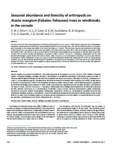
Chapter 2 7. Dorsal fin of temporarily captured and released bottlenose dolphin with radio transmitter mounted within bullet tag ……………….................. 38 8.
Geographic tracking area covered by aerial, vehicle and vessel………… 40
9.
Capture locations for all 24 radio tagged animals during 2005 and 2006 ………………………………………………………………………. 45
10a.
Utilization areas of individually tagged dolphins from 2005 ……………… 47
10b.
Utilization areas of individually tagged dolphins from 2006 ……………… 47
xiii
LIST OF FIGURES Figure
Page
11.
X05’s sighting history from photo identification and radio tracking effort during 2004, 2005, and 2006 ……...…………………………………………49
12.
Utilization areas of individually tagged dolphins excluded from discussion..………..……………………………………………………...50
13a.
Proportion of time tagged individuals from 2005 spent within St. Joseph Bay region ……………………………………………………….. 54
13b.
Proportion of time tagged individuals from 2006 spent within St. Joseph Bay region ……………………………………………………….. 54
xiv
CHAPTER 1. SEASONAL ABUNDANCE AND SITE-FIDELITY OF BOTTLENOSE DOLPHINS IN ST. JOSEPH BAY, FLORIDA INTRODUCTION In 1999, 2004, and 2005, along the Florida Panhandle, bottlenose dolphins (Tursiops truncatus) experienced three mass mortality events in which over 300 individuals died, in total (Anonymous 2004; pers. comm. NMFS Panama City). These events were identified as “Unusual Mortality Events” (UMEs) because of their distinct dissimilarity to normal stranding patterns (Marine Mammal Protection Act, 1972). The 1999 and 2004 UMEs appear to have been spatially and temporally correlated with blooms of Karenia brevis, the dinoflagellate known to cause red tide in Florida (Anonymous 2004). All three UMEs occurred over periods of multiple months, and impacted the St. Joseph Bay region, in Gulf County, Florida. Saint Joseph Bay was the geographic focus of the 2004 UME. The most recent abundance estimate of bottlenose dolphins within Saint Joseph Bay, based upon aerial surveys flown by National Oceanic and Atmospheric Administration (NOAA) in September-November 1994, is zero (Waring et al. 2000). This estimate is considered obsolete from a management perspective, and it clearly does not reflect changes that might have occurred from the UMEs. Thus, there exists a critical need for enhanced understanding of the abundance of dolphins residing in this region. Bottlenose dolphins are widely distributed throughout the coastal waters of the Gulf of Mexico (Hubard 1998; Irvine et al. 1981; Mullin 1988; Scott et al. 1989; Shane 1977; Shane 1990a; Weller 1998). Currently, groups of bottlenose dolphins that inhabit each bay and estuary in the northern Gulf region are defined
by NOAA as separate communities (Anonymous 2005). Wells et al. (1987) defined a community as a group of resident animals that share home ranges, display similar genetic features, and interact more frequently with each other than with dolphins in adjacent waters. To date, little is known about the bottlenose dolphin communities in the northern Gulf waters of the Florida Panhandle. Bottlenose dolphin abundance and distribution patterns may be correlated to changes in water temperature and productivity (Quinn and Brodeur 1991). For example, Barco et al. (1999) demonstrated that abundance of Atlantic coastal bottlenose dolphins along the nearshore waters of Virginia Beach was positively correlated to water temperature. Along the northern Gulf region, seasonal fluctuations in dolphin abundance have been observed. In San Luis Pass, Texas, some bottlenose dolphins move into Gulf of Mexico waters during fall/winter, and back into bays and estuaries during spring/summer (Maze 1997). Increased abundance of bottlenose dolphins during fall and winter has been observed in Aransas Pass, Texas (Shane 1977; Weller 1998). Spring and summer increases in dolphin abundance have been observed in Galveston Bay, Texas (Bräger 1993; Fertl 1994; Henningsen 1991), and Mississippi Sound (Hubard 1998). In contrast, a relatively stable, resident community of bottlenose dolphins has been identified in Sarasota Bay, Florida (Irvine et al. 1981; Wells 1986; Wells et al. 1987). Currently, seasonal movements of coastal dolphins in the St. Joseph Bay region of the Florida Panhandle are unknown. Understanding the seasonal movements of bottlenose dolphins along the Florida Panhandle is important when evaluating the impacts of the three recent
2
UMEs. These UMEs have occurred across multiple seasons; from August 1999 through February 2000, March through April 2004, and September 2005 through April 2006. If dolphins have high year-round site-fidelity in the St. Joseph Bay region, they were likely negatively affected by each UME. If dolphin abundance fluctuates seasonally, as suggested for other regions in the northern Gulf of Mexico, the effects of these UMEs may be more widespread among other dolphin groups only sighted seasonally in the St. Joseph Bay region. Estimating the number of individuals and detecting trends in abundance are critical steps in establishing effective management plans (Taylor and Gerrodette 1993). Systematic surveys and mark-recapture methods utilizing photographically-identified individuals have yielded insights into patterns of bottlenose dolphin abundance and site-fidelity in other geographic regions (e.g. Barco et al. 1999; Maze and Würsig 1999; Read et al. 2003; Seber 1982; Shane 1990a, 1990b, 1980; Wells 1986; Williams et al. 1993; Wilson et al. 1999; Würsig and Würsig 1977). There are many questions about the validity of using aerial survey data for determining abundance of inshore bottlenose dolphins. Markrecapture photo-identification surveys provide an improved approach for Florida panhandle abundance estimates. Thus, the goals of this study were to use photo-identification surveys to (1) estimate seasonal abundance, with both closed and robust population models in the programs MARK and CAPTURE (Rexstad and Burnham 1992; White et al. 1982), and (2) examine site-fidelity patterns of individuals using multiple photo-identification efforts. Ambient water temperature data were collected to investigate the relationship between dolphin
3
abundance and this environmental parameter. These techniques were used to investigate bottlenose dolphins that are currently residing in and around St. Joseph Bay, Florida, an area that has been affected by multiple UMEs.
METHODS Study Area St. Joseph Bay is centrally located along the Florida Panhandle. The study area includes the Gulf waters from Cape San Blas northwest to Crooked Island Sound, including the estuaries of Crooked Island Sound and St. Joseph Bay (Figure 1). St. Joseph Bay is approximately 21km long and 10km across at its widest. The depth inside the bay ranges from 1m or less in the southern quarter of the bay to 10-12m in the northwest region along St. Joseph Peninsula. The Gulf coastal waters to the northwest and south of St. Joseph Bay have a gradually changing depth, and sand bars are located approximately 500m offshore of all coastlines. The northern extent of the study site, Crooked Island Sound, is approximately 12km in length with a maximum width of 2km. The depth inside the sound ranges from 1m at the fringes to 6-7m at the entrance. The entrance to Crooked Island Sound has several sandbars that shift positions irregularly. The southern extent of the study site is Cape San Blas, at the tip of St. Joseph Peninsula, with varying depths from 1-7m due to shifting sandbars.
4
Figure 1. St. Joseph Bay and surrounding Gulf waters from Cape San Blas north to Crooked Island Sound.
5
Mark-recapture field methods Mark-recapture surveys were conducted during February/March, April, May, and July 2005, as well as February and September/October 2006. During each period, two surveys of the study area were completed using the following transect design. Contour transect surveys, extending from Cape San Blas northwest to the entrance of Crooked Island Sound, were used to cover the Gulf waters at distances of 0.5 km and 1.5 km from the coastline (Figure 2). Inside Crooked Island Sound, a contour transect at a distance of 0.5 km from the shoreline was implemented. St. Joseph Bay was divided into 18 east-west line transects, spaced 1 km apart (Figure 2). A contour transect following the shallow finger channels was used in the southern corner of the bay. All transects were completed in as short a period of time as possible, to allow for the assumption of a closed population (Read et al. 2003). The mean completion period of each mark-recapture survey was 4.1 + 0.8 S.D. days. The mark and recapture periods were separated by a mean of 1.2 + 0.4 S.D. days. All transects, which were selected at random using a random number selector in Microsoft Access (Microsoft Corp., Redmond, WA), were completed in a Beaufort Sea State (BSS) of 3 or less to optimize sightability. A dolphin sighting was recorded when any dolphin was encountered during a survey. Total number of animals, including neonates, and environmental data including salinity, water temperature, cloud cover, BSS, depth, and geographic location were recorded for each sighting. Characteristics used to identify neonates were a body size less than half of the adult, dark color,
6
Figure 2. Line and contour transects used for mark-recapture photo-identification surveys of bottlenose dolphins in February/March 2005, April 2005, May 2005, July 2005, February 2006, and September/October 2006.
7
floppy dorsal fin, high level of buoyancy, rostrum-first surfacings, and echelon swimming position (reviewed in Dearolf et al. 2000; Thayer et al. 2003). Digital photographs were obtained of all individuals in a sighting using a Nikon D-100 camera with 70-300m lens. All photographs from daily surveys were downloaded onto a laptop computer. Dorsal fin images were cropped (ACDSee 7.0, ACD Systems, British Columbia, Canada) and graded on both distinctiveness of the dorsal fin, and photographic quality, based on the methods of Urian et al. (1999). The distinctiveness (D) rating focused primarily on the nicks along the trailing edge of the dorsal fin and ranged from 1-3. Dolphins were given a D1 rating if their fin features were distinctive and most were still observable in poor quality photos. A D2 rating was given to individuals with intermediate features (at least two distinguishing fin characteristics). D3 animals were those with few to no distinguishing characteristics. The photographic quality (Q) rating focused on clarity, contrast, and angle of the fin to the photographer. A Q1 rating was given to a dorsal fin picture that was in perfect focus and that filled the field of the image. A Q2 rating was given when the image was still sharply focused but the fin occupied a smaller portion of the image. Q3 photos were those in which only a portion of a fin was included in the image or when the fin was not in sufficient focus. Two judges scored each image, one graded distinctiveness (BCB), the other graded quality (SMN).
8
A catalog of all fins was created in which each individual received a unique number based on the location of its distinctive markings along the trailing edge of its fin. A fin could be added to the catalog under two conditions. First, the fin had to have a photo rating of Q1 and a D1 or D2. This rating ensured that the animal would be correctly identified in future sightings. Second, the fin could enter the catalog if it was identified as a Q2 and D2 on two separate survey days. This condition guaranteed that there would be enough images to successfully identify the animal in future sightings. After completion of photo analysis, a ratio of distinctive to non-distinctive (“clean”) dolphins photographed in every sighting was determined to estimate the proportion of marked versus unmarked animals during each survey season- this is referred to as the distinctiveness rate. In this study, a mark is considered a photograph of an individual dolphin’s dorsal fin (Read et al. 2003; Urian and Wells 1996; Wells et al. 1996b; Williams et al. 1993; Wilson et al. 1999).
Mark-recapture data analysis
Abundance estimates using closed population models When photographic mark-recapture methods are used to study bottlenose dolphin populations, the four assumptions of the closed, mark-recapture model (Seber 1982) can be met if the sampling period is short (Read et al. 2003), as described below. (1) Demographically and geographically closed population - Bottlenose dolphins have low reproductive rates and high survival rates ensuring a low level of births
9
and deaths during a short sampling interval (Connor et al. 2000; Read et al. 2003; Wells et al. 1996a; Wells et al. 1997; Wells and Scott 1999; Wells et al. 1996b). Coastal bottlenose dolphin populations can display seasonal movement patterns on the Atlantic and Gulf coasts, preventing full geographic closure (e.g. Barco et al. 1999; Read et al. 2003; Torres et al. 2003; Wells 1991; Wells et al. 1996a; Wells et al. 1997). However, during a short sampling period, immigration and emigration in the region are likely to remain at a relatively low level (Read et al. 2003). For example, Read et al. (2003) utilized a sampling period of 24 days to ensure minimal movement of bottlenose dolphins into and out of the nearshore waters of North Carolina. (2) Homogeneity of capture probabilities - Heterogeneity for photo-identification studies would require that individual dolphins respond differently to boats. Coastal bottlenose dolphins encounter boats on a regular basis, and an approaching boat taking photographs is unlikely to change their behavior, allowing for homogeneity in capture probability (Hammond 1990; Read et al. 2003). (3) Marks are recognized on recapture - This assumption requires that the distinctive nicks and notches that identify an individual will be recognized upon resighting. Read et al. (2003) tested photographic quality and mark distinctiveness for all photographs taken during recapture surveys. By limiting dorsal fins to those with only intermediate or greater distinctiveness values and good to excellent photo-identification scores, Read et al. (2003) correctly identified all resighted individuals with a 95% confidence.
10
(4) Marks are not lost during the study – Although bottlenose dolphin dorsal fins can change in appearance over time (Wells and Scott 1990), nicks and notches along the trailing and leading edges of dorsal fins are considered long lasting, if not permanent marks (Whitehead et al. 2000; Wilson et al. 1999). Five closed population models were used to estimate the abundance of bottlenose dolphins in the St. Joseph Bay study area during each survey period. The first, the Chapman modification of the Lincoln-Petersen model, strictly follows the four assumptions of a closed population (Chapman 1951; Seber 1982; Thompson et al. 1998). It requires sampling without replacement, which means that once an animal is sampled during the recapture, it can not be counted again if resighted (Chapman, 1951; reviewed in Thompson et al., 1998). For each survey period, the sighting histories for all individuals were divided into two separate sampling occasions of equal survey effort, the mark (n1) and the recapture (n2). Each (n) refers to the total number of individuals identified during the mark and recapture sampling periods. The number of individuals seen in both the mark and recapture sampling occasions were then counted (m2). The abundance estimate (Nc), variance (var Nc), and standard error (SE) of the Chapman modification to the Lincoln-Petersen model were calculated as (Chapman 1951): (1)
(2)
(3)
Nc =
var Nc =
( n1 + 1)(n 2 + 1) −1 ( m 2 + 1)
( n1 + 1)( n 2 + 1)( n1 − m 2)( n 2 − m 2 ) ( m 2 + 1) 2 ( m 2 + 2)
SE = var Nc
11
The remaining closed population models used in this study permit the relaxing of one or more of the closed population assumptions. Each of the six survey seasons was divided into three periods of equal survey effort to increase the precision from a two-sample to three-sample model. As the number of sampling occasions increase, the variation between estimates decreases (Thompson et al. 1998). With less variation, more precise abundance estimates can be obtained (Thompson et al. 1998). Numerous models within the program CAPTURE (Rexstad and Burnham 1992; White et al. 1982) have been created to allow for heterogeneity in capture probabilities by individual (Mh), behavioral capture response (Mb), and capture/recapture time (Mt) (Thompson et al. 1998). These models have also been combined to form more complex models that incorporate more than one exception to the assumptions of a closed population model (e.g. Mth, Mtb, and Mbh) (Thompson et al. 1998). These models can be compared to the null model, Mo, which is similar to the Lincoln-Petersen model, and assumes that all individuals have an equal capture probability, and that marked animals have the same recapture probability as unmarked animals (Darroch 1958; reviewed in Otis et al. 1978). For each survey period, the abundance estimate and standard error were calculated in the program CAPTURE within the program MARK (Rexstad and Burnham 1992; White et al. 1982). Four models were selected to estimate abundance; Mo, Mh, Mt, Mth. The behavioral models (e.g., Mb, Mtb, Mbh) were rejected because they assume there is a behavioral response to capture. The behavioral models primarily are used in removal studies, where animals are
12
taken out of the study area after they are recaptured, and are, thus, not suitable for abundance estimates of bottlenose dolphins. Model Mh assumes each animal has its own capture probability and capture probabilities do not change over time (Burnham and Overton 1978, 1979; reviewed in Thompson et al. 1998). This model takes into account different capture probabilities that may occur due to demographic variations, such as age or sex of individual animals (Burnham and Overton 1978, 1979; reviewed in Thompson et al. 1998). Model Mt assumes capture probabilities vary by sample period but all animals have an identical capture probability within sampling period (Burnham and Overton 1978, 1979; Darroch 1958; reviewed in Otis et al. 1978). In this model, marked animals are considered to have the same capture probabilities as unmarked individuals. Model Mth is a combination of the Mt and Mh models allowing for animals to have their own capture probability and that capture probability varies with time. This model is useful since it generates an abundance estimate with a decreased number of closed population model assumptions. However, as the number of closed population assumptions are reduced, variance in abundance estimates is increased (Thompson et al. 1998).
Abundance estimates using robust population models Closed population models can allow for heterogeneity in capture probability and are useful in providing abundance estimates when there are limited data (Pine et al. 2003). However, due to the strict constraints of a closed population model, studies must be limited to a short period of time (reviewed in
13
Pine et al. 2003). The Jolly-Seber, or open population model, allows for variation in survival/emigration and births/immigration to obtain abundance estimates (Jolly 1965; Seber 1965; Thompson et al. 1998). However, abundance estimates are not as reliable in an open model as in a closed model for two reasons. First, by having fewer closed population assumptions, the abundance estimates are less precise (Thompson et al. 1998). Second, the open population model relies solely on Model Mt for abundance estimation, and does not include capture heterogeneity (Thompson et al. 1998). The robust design model (Pollock 1982) uses characteristics of closed population abundance estimates and open population survival/emigration estimates (Kendall et al. 1997; reviewed in Pine et al. 2003; Pollock 1982; Thompson et al. 1998). This approach allows for abundance estimates to be determined during multiple, short term periods with closed population models (Mo, Mh, Mt, Mth) (reviewed in Pine et al. 2003; Pollock 1982) and uses the JollySeber open population model to estimate survivorship, emigration rates, and capture-recapture probabilities between the short term survey periods (reviewed in Pine et al. 2003; Pollock 1982). Three separate robust design models were used to determine abundance (Kendall et al. 1997). The “No Emigration” model assumes there is no emigration or immigration between survey periods. The “Random Emigration” model sets emigration and immigration equal to each other across survey periods. In random emigration, an animal is assumed to randomly leave and return to the study area on a recurrent basis (reviewed in Pine et al. 2003). The “Markovian
14
Emigration” model permits unequal emigration and immigration rates across survey periods (Kendall et al. 1997). This model assumes that an animal “remembers” that is has left the study area, and returns based on a timedependent function (reviewed in Pine et al. 2003).
Photo-identification site-fidelity methods Bottlenose dolphin photo-identification efforts in the St. Joseph Bay region began in April 2004 following the UME with a preliminary study to obtain genetic samples through biopsy darting. To date there have been 138 days of photoidentification effort, covering thirteen months between April 2004 and October 2006. Photo-identification effort included mark-recapture surveys (this study), biopsy dart sampling, and radio tracking of individuals that were investigated during two capture-release health assessment studies carried out by NOAA and its partners, in April 2005 and July 2006 (Chapter 2). Due to the constraints of population modeling, seasonal abundance estimates were derived solely from the mark-recapture survey data, as previously described. However, in assessing site-fidelity, all photo-identification effort was used. To define a site-fidelity index for individual dolphins in the St. Joseph Bay region, the total number of sightings of each cataloged animal was determined from all photo-identification effort. During each survey period, each individual was grouped into one of five bins based on its total number of sightings. To determine the correct binning during each survey period, a density estimator was utilized based on Freeman and Diaconis (1981). This density estimator was
15
used to statistically determine bin size as opposed to arbitrarily separating the number of sightings into equally spaced divisions. For each survey period, the 25th and 75th quartiles were calculated for the total number of sightings of all identifiable individuals. The two quartiles were then subtracted to determine the interquartile range (IQR). The IQR was then multiplied by two and divided by the cube root of the total number of individuals sighted (n) during the survey period to determine the bin size. BIN SIZE =
(4)
2 * ( IQR) 3 n
Each individual sighted during a given survey period was placed into the bin that included all of the individual’s sightings throughout the three years of photoidentification effort. A single factor analysis of variance (ANOVA) was used to identify if site-fidelity varied by season. A Kolmogorov-Smirnov two-sample test was then used to determine if sighting distributions also varied by season (Sokal and Rohlf 1995).
Water temperature data Surface water temperature data were obtained from the National Data Buoy Center (Stennis Space Center, MS). The water temperature data used in this study were from Station PCBF-1 in Panama City Beach, FL, approximately 19 km NW of the St. Joseph Bay photo-identification region. Average water temperatures were determined for the exact days of survey effort during each survey period. These averages were then plotted against abundance estimates determined from the Lincoln-Petersen model.
16
RESULTS Mark-recapture abundance estimates Between April 2004 and October 2006, a total of 305 individual bottlenose dolphins were identified in the St. Joseph Bay region of the Florida Panhandle. The discovery curve of new individuals increased steeply until May 2005 and more gradually thereafter (Figure 3). The largest number of identifiable individuals was sighted during May 2005, which included 129 animals sighted from previous surveys and 73 newly identifiable animals (Figure 3). The number of identifiable animals sighted during a survey season ranged from 47 to 202 (Table 1). The mean rate of distinctiveness across all seasons was 0.81 + .07 S.D. (Table 1). The number of identifiable individuals and the distinctiveness rate were used to estimate the total number of individuals (marked and unmarked) during each survey period (Table 1). Closed population models (Lincoln-Petersen, Mo, Mh, Mt, and Mth) were used to estimate dolphin abundance during each survey period (Table 2, Figure 4a). All models estimated the highest abundances in May 2005 followed by September/October 2006, and the lowest abundances in July 2005 and February 2006. Robust design models were used to estimate abundance during each survey period, incorporating variation in emigration/survivorship, and capture/recapture probability (Table 3, Figure 4b). These models showed similar temporal patterns of abundances as the closed population models.
17
350
300
Number of individuals
250
200
# of previously identified individuals # of new individuals
150
# of individuals in catalog
100
50
0 Apr 04
May 04
Dec 04
Feb 05
Mar 05
Apr 05
May 05
Jun 05
Jul 05 Nov 05
Feb Jul 06 Aug 06 06
Sep 06
Oct 06
Survey month
Figure 3. Number of individuals sighted during all photo-identification efforts and discovery curve for bottlenose dolphins in the St. Joseph Bay region.
18
LP
Mo
Mh
Mt
Mth
600
Number of Individuals
500 400 300 200 100 0 Feb/Mar-05
Apr-05
May-05
Jul-05
Feb-06
Sep/Oct-06
Survey Period
Figure 4a. Closed population abundance estimates [Lincoln-Petersen (LP), Mo, Mh, Mt, and Mth] with standard error during each survey period. Markovian
Random
No Emigration
600
Number of Individuals
500 400 300 200 100 0 Feb/Mar-05
Apr-05
May-05
Jul-05
Feb-06
Sep/Oct-06
Survey Period
Figure 4b. Robust model, abundance estimates with standard error of bottlenose dolphins in the St. Joseph Bay region during each survey period; Markovian, Random Emigration, and No Emigration.
19
Field Season: Feb/Mar2005 Number of Identified 122 (distinctively marked) dolphins sighted Mark/Distinctiveness 0.88 Rate Estimate of Total 139 Marked + Unmarked Dolphins
Apr-05
May-05
Jul-05
Feb-06
Sep/Oct2006
144
202
83
47
176
0.79
0.85
0.85
0.68
0.84
183
238
98
69
210
Table 1. Number of identified animals sighted, distinctiveness rate, and estimate of total number of dolphins during each mark-recapture survey season. Field Feb/MarSeason: 2005 LP 158 + 16 Mo 147 + 11 Mh 188 + 26 Mt 157 + 16 Mth 242 + 65
Apr-05
May-05
Jul-05
Feb-06
240 + 40 232 + 31 307 + 57 237 + 36 282 + 79
313 + 10 279 + 21 362 + 43 286 + 26 410 + 89
104 + 13 115 + 15 127 + 21 101 + 12 105 + 16
113 + 28 98 + 19 125 + 33 95 + 20 105 + 39
Sep/Oct2006 237 + 20 303 + 37 388 + 63 295 + 39 337 + 79
Table 2. Abundance estimates with standard error for each survey period using closed population models (Lincoln-Petersen, Mo, Mh, Mt, and Mth). Field Season: Markovian Random No Emigration
Feb/Mar2005 153 + 14 153 + 14 265 + 27
Apr-05
May-05
Jul-05
Feb-06
240 + 33 228 + 26 299 + 30
276 + 21 275 + 19 460 + 42
104 + 12 121 + 16 178 + 21
81 + 11 110 + 19 126 + 16
Sep/Oct2006 295 + 36 272 + 27 376 + 36
Table 3. Abundance estimates with standard error for each survey period using robust design models (Markovian, Random Emigration, No Emigration).
20
Photo-identification site-fidelity For each survey period, all identified individuals were grouped into one of five sighting bins (i.e. site fidelity indices): (1 – 8), (9 – 17), (18 – 26), (27 – 35), and (36+). To identify if site-fidelity indices varied across seasons, histograms were plotted from one survey period within each season; spring (May 2005), summer (July 2005), fall (September/October 2006), and winter (February 2006) (Figures 5a – 5d). In May 2005 and September/October 2006, greater than 50% of the individuals were sighted only one to eight times. In contrast, during July 2005 and February 2006, over 50% of the individuals were sighted between 9 – 17 and 18 – 26 times. The results from the ANOVA suggested site-fidelity did change seasonally in the St. Joseph Bay region (p < .01). However, during the seasons in which sighting distributions would have been expected to be similar, May 2005 and September/October 2006, and July 2005 and February 2006, the Kolmogorov-Smirnov test determined all distributions to be significantly different.
Water temperature data A positive correlation between dolphin abundance and water temperature was observed during the spring months (February/March, April, and May 2005) (Figure 6). At the upper and lower temperature thresholds for the region, during mid-summer and winter (July 2005, and February 2006), abundance estimates were at their lowest values. During the fall (September/October 2006), as water temperature began to decrease, abundance estimates were elevated.
21
70.0
Frequency sighted (%)
60.0 50.0 40.0 30.0 20.0 10.0 0.0 (1-8)
(9-17)
(18-26)
(27-35)
(36+)
Number of sightings
Figure 5a. Frequency of individuals sighted during May 2005 survey period. 70.0
Frequency sighted (%)
60.0 50.0 40.0 30.0 20.0 10.0 0.0 (1-8)
(9-17)
(18-26)
(27-35)
(36+)
Number of sightings
Figure 5b. Frequency of individuals sighted during July 2005 survey period. 70.0
Frequency sighted (%)
60.0 50.0 40.0 30.0 20.0 10.0 0.0
(1-8)
(9-17)
(18-26)
(27-35)
(36+)
Number of sightings
Figure 5c. Frequency of individuals sighted during September/October 2006 survey period. 70
Frequency sighted (%)
60 50 40 30 20 10 0 (1-8)
(9-17)
(18-26)
(27-35)
(36+)
Number of sightings
Figure 5d. Frequency of individuals sighted during February 2006 survey period.
22
Average Water Temp
35
300
30
250
25
200
20
150
15
100
10
50
5
0
0
o
350
Temperature ( C)
Number of individuals
Abundance estimate (LP)
Feb/Mar- Apr-05 May-05 05
Jul-05
Feb-06 Sep/Oct06
Survey Period
Figure 6. Water temperature data in relation to abundance estimates from the Lincoln-Petersen model (LP).
23
DISCUSSION The goals of this study were to estimate dolphin abundance and describe site-fidelity patterns across seasons in a geographic region recently affected by several UMEs. Overall, the closed population models produced similar abundance estimates throughout all survey periods (Table 2, Figure 4a). The similarities between the Lincoln-Petersen and null model are expected since these two models strictly follow the assumptions of a closed population. It is interesting that Model Mt, which permits capture probabilities to vary across sample period, but not across individuals, produced abundance estimates that were very similar to these two models. Abundance estimates derived from models Mh and Mth tended to be higher than those of other models during the spring and fall survey periods, but similar to them in summer and winter. These models permit each individual to have its own capture probability, but this probability does not change across survey periods. Data on site-fidelity patterns (discussed below) demonstrate that individual dolphin availability within the region does vary across seasons. Many dolphins sighted in spring and fall are unlikely to be seen in the region in summer and winter. Thus, the increased abundance estimates in spring and fall from these models may be attributed to individual differences in capture probability across survey periods or may be attributed to the violation of the models’ assumptions. Abundance estimates determined from the “Markovian” and “Random” models were similar within each survey season (Table 3, Figure 4b). Both of
24
these models allow for immigration and emigration to occur across survey periods. In contrast, the “No Emigration” model, which prohibits immigration or emigration across survey sessions, generated higher abundance estimates than the other two robust models. Again, this pattern was particularly evident during periods with the highest abundance levels (May 2005 and September/October 2006). During these periods, overall site-fidelity indices are low suggesting an influx of individuals into the study area and thereby violation of this model’s assumption. Irrespective of how abundance was estimated, whether from direct counts of dolphins from photo-identification, or from each of the closed or open population models, each demonstrated that abundance varied across survey periods. Dolphin numbers increased between February/March 2005 and May 2005 survey periods. The abundance estimates declined precipitously between May and July 2005, and remained low in February 2006. Abundance estimates were then elevated again during September/October 2006. These data strongly suggest spring and fall movements of dolphins into the St. Joseph Bay region, similar to patterns seen in other study sites within the northern Gulf of Mexico (Bräger 1993; Fertl 1994; e.g. Henningsen 1991; Hubard 1998). The sighting history data, which are temporally correlated with the abundance estimates, provide insight into site-fidelity patterns in the St. Joseph Bay region. Beginning in February/March and continuing through April 2005, there was a significant increase in the number of individuals that displayed low indices of site-fidelity. In May 2005, when dolphin abundance estimates were highest, the percentage of individuals with low site-fidelity (1-8 sightings) was
25
also highest (Figure 5a). In contrast, in July 2005 and February 2006, when abundance estimates were lowest, the majority of individuals sighted were those with moderate to high indices of site-fidelity (9 - 17, and 18 - 26 sightings) (Figure 5b and 5d). During September/October 2006 the percentage of individuals with low site-fidelity (1-8 sightings) increased again as overall abundance increased (Figure 5c). These results suggest that during spring and fall most dolphins sighted are visitors to the St. Joseph Bay region. In contrast, bottlenose dolphins seen in the winter and summer months are more likely to be sighted year-round. Coastal bottlenose dolphin communities that have been studied in other regions tend to be composed of approximately 60 to 150 individuals (Wells 1991; Williams et al. 1993; Wilson et al. 1999). For example, the bottlenose dolphin community in Sarasota Bay, Florida, has an estimated community size of approximately 155 individuals (Wells 1991; Wells, pers. comm.). In the St. Joseph Bay region, during winter and summer, when the majority of dolphins display moderate to high site-fidelity indices, abundance estimates ranged from 89 to 158 individuals. These results suggest that individuals sighted during winter and summer months may form a St. Joseph Bay dolphin community. Dolphin abundance increased in association with an increase in water temperature during spring and with a decrease in water temperature during fall (Figure 6). Thus, seasonal changes in water temperature in spring and fall are correlated with the influx of animals into the study area. Barco et al. (1999) also found a relationship between dolphin abundance and water temperature along the coast of Virginia. These authors hypothesized that this relationship was likely
26
based on changes in prey abundance but found no positive correlation. However, Barco et al. (1999) noted several difficulties that prevented adequate sampling of dolphin prey availability. In contrast to fall and spring, abundance is lowest during winter and summer when water temperatures are at their peaks. These patterns suggest that temperature is likely not important in determining abundance of animals with high site-fidelity to the St. Joseph Bay region. Future research is needed in the St. Joseph Bay region to help determine potential causes of these changes in seasonal abundance.
Unusual Mortality Events and future management Along the Atlantic coast of the United States, between June 1987 and March 1988, bottlenose dolphins experienced an unusual mortality event resulting in 742 strandings (Scott et al. 1988). There have been approximately ten years of research, since this event, investigating the recovery of the Atlantic coastal bottlenose dolphin stocks(s) potentially impacted from this UME (Hohn 1997; McLellan et al. 2002; Read et al. 2003; Urian et al. 1999). Currently, however, the stock structure and overall UME impact are still not completely understood (McLellan et al. 2002; Waring et al. 2000). Because there had been little research carried out on bottlenose dolphins along the Florida Panhandle prior to the three UMEs, the data from this study are the first to describe seasonal abundance estimates and site-fidelity patterns in this region. The 2004 UME may have had the greatest local impact on the St. Joseph Bay region, as 70% of the mortalities (75 individuals) occurred within or
27
just outside of St. Joseph Bay (Anonymous 2004). The 2004 UME was also of the shortest duration, spanning approximately one month between March and April. The results from this study suggest that the 2004 UME occurred at a time of year when local abundance within the region may have been increasing (Figure 4a and 4b). Thus, both individuals with high site-fidelity in the St. Joseph Bay region, as well as dolphins moving into the region, may have been impacted by this event. UMEs that occur along this region of the Florida Panhandle in spring and fall may have a much wider regional effect than those that occur in summer and winter when abundance levels are lower. UMEs that occur during summer and winter will likely have a greater effect on individuals forming a resident St. Joseph Bay dolphin community. In the St. Joseph Bay region, dolphin abundance increases during the spring and fall. The majority of individuals sighted during these time periods are those with low site-fidelity. In contrast, during the winter and summer, abundance estimates are lower and individuals demonstrate higher site-fidelity. Future research is necessary to determine if the results of this study are similar to other regions of the Florida Panhandle. Systematic surveys similar to the mark-recapture surveys conducted in this study, along other regions of the Florida Panhandle would be valuable. Similarly, continued analyses of genetic samples from biopsy darting live individuals as well as stranded animals would provide additional insight into northern Gulf stock structure. Determining movement patterns of individuals with both high and low site-fidelity to the St. Joseph Bay region, and identifying the direct factors (foraging, reproductive, etc.)
28
that cue seasonal abundance increases in the St. Joseph Bay region would provide a better understanding of community structure of coastal bottlenose dolphins along the entire Florida Panhandle.
29
REFERENCES 1972. Marine Mammal Protection Act. ANONYMOUS. 2004. Interim Report on the Bottlenose dolphin (Tursiops truncatus) Unusual Mortality Event Along the Panhandle of Florida MarchApril 2004. ANONYMOUS. 2005. NOAA Stock Assessment Report; Bottlenose dolphin (Tursiops truncatus): Gulf of Mexico Bay, Sound, and Estuary Stocks. BARCO, S. G., W. M. SWINGLE, W. A. MCLELLAN, R. N. HARRIS, AND D. A. PABST. 1999. Local abundance and distribution of bottlenose dolphins (Tursiops truncatus) in the nearshore waters of Virginia Beach, Virginia, Marine Mammal Science 15:394-408. BRÄGER, S. 1993. Diurnal and seasonal behavior patterns of bottlenose dolphins (Tursiops truncatus), Marine Mammal Science 9:434-440. BURNHAM, K. P., AND W. S. OVERTON. 1978. Estimation of the size of a closed population when capture probabilities vary among animals, Biometrika 65:625-633. BURNHAM, K. P., AND W. S. OVERTON. 1979. Robust estimation of population size when capture probabilities vary among animals, Ecology 60:927-936. CHAPMAN, D. G. 1951. Some properties of the hypergeometric distribution with application to zoological censuses, Univ. Calif. Publ. Stat. 1:131-160. CONNOR, R. C., R. S. WELLS, J. MANN, AND A. J. READ. 2000. The bottlenose dolphin: Social relationships n a fission-fusion society, Pp. 91126 in Cetacean societies: Field studies of dolphins and whales (J. Mann, R. C. Connor, P. L. Tyack and H. Whitehead, eds.). University of Chicago Press, Chicago. DARROCH, J. N. 1958. The multiple recapture census: I. Estimation of a closed population, Biometrika 45:343-359. DEAROLF, J. L., W. A. MCLELLAN, R. M. DILLAMAN, D. J. FRIERSON, AND D. A. PABST. 2000. Precocial development of axial locomotor muscle in bottlenose dolphins (Tursiops truncatus), Journal of Morphology 244:203215. FERTL, D. C. 1994. Occurence, movements, and behavior of bottlenose dolphins (Tursiops truncatus) in association with the shrimp fishery in Galveston Bay, Texas, M. Sc. thesis, Texas A&M University. FREEDMAN, D., AND P. DIACONIS. 1981. On the histogram as a density estimator: L2 theory, Zeitschrift fur Wahrscheinlichkeitstheorie 57:453-476. HAMMOND, P. S. 1990. Capturing whales on film-estimating cetacean population parameters from individual recognition data, Mammalian Review 20:17-22. HENNINGSEN, T. 1991. Zur Verbreitung und Okologie des GroBen Tummlers (Tursiops truncatus) in Galveston, Texas, Diploma thesis, ChristianAlbrechts-Universitat, Kiel, Germany. HOHN, A. A. 1997. Design for a multiple method approach to determine stock structure of bottlenose dolphins in the mid-Atlantic, NOAA Technical Memorandium NMFS-SEFSC-401.
30
HUBARD, C. W. 1998. Abundance, distribution and site fidelity of bottlenose dolphins in Mississippi Sound, Mississippi, M. Sc. thesis, University of Alabama. IRVINE, A. B., M. D. SCOTT, R. S. WELLS, AND J. H. KAUFMANN. 1981. Movements and activities of the Atlantic bottlenose dolphin, Tursiops truncatus, near Sarasota, Florida., Fishery Bulletin 79:671-688. JOLLY, G. M. 1965. Explicit estimates from capture-recapture data with both death and immigration-stochastic model, Biometrika 52:225-247. KENDALL, W. L., J. D. NICHOLS, AND J. E. HINES. 1997. Estimating temporary emigration using capture-recapture data with Pollock's robust design, Ecology 78:563-578. MAZE, K. S. 1997. Bottlenose dolphins of San Luis Pass, Texas: Occurrence patterns, site fidelity, and habitat use, M.Sc. thesis, Texas A&M University. MAZE, K. S., AND B. WÜRSIG. 1999. Bottlenose dolphins of San Luis Pass, Texas: Occurance patterns, site-fidelity, and habitat use, Aquatic Mammals 25.2:91-103. MCLELLAN, W. A., A. S. FRIEDLAENDER, J. G. MEAD, C. W. POTTER, AND D. A. PABST. 2002. Analysing 25 years of bottlenose dolphin (Tursiops truncatus) strandings along the Atlantic coast of the USA: do historic records support the coastal migratory stock hypothesis?, Journal of Cetacean Resource Management 4:297-304. MULLIN, K. D. 1988. Comparative seasonal abundance and ecology of bottlenose dolphins (Tursiops truncatus) in three habitats of the northcentral Gulf of Mexico, Ph. D. dissertation, Mississippi State University. OTIS, D. L., K. P. BURNHAM, G. C. WHITE, AND D. R. ANDERSON. 1978. Statistical inference from capture data on closed populations, Wildlife Monographs 62:1-135. PINE, W. E., K. H. POLLOCK, J. E. HIGHTOWER, T. J. KWAK, AND J. A. RICE. 2003. A review of tagging methods for estimating fish population size and components of mortality, Fisheries 28:10-23. POLLOCK, K. H. 1982. A capture-recapture design robust to unequal probability of capture, Journal of Wildlife Management 46:757-760. QUINN, T., AND R. BRODEUR. 1991. Intra-specific variation in the movement patterns of marine mammals, American Zoologist 31:231-241. READ, A. J., K. W. URIAN, B. WILSON, AND D. M. WAPLES. 2003. Abundance of bottlenose dolphins in the bays, sounds, and estuaries of North Carolina, Marine Mammal Science 19:59-73. REXSTAD, E. A., AND K. P. BURNHAM. 1992. User's guide for interactive program CAPTURE, Colorado Coop. Fish and Wildl. Res. Unit, Colorado State University, Fort Collins. SCOTT, G. P., D. M. BURN, AND L. J. HANSEN. 1988. The dolphin die-off; long term effects and recovery of the population, Proc. Oceans 88:819-823. SCOTT, G. P., D. M. BURN, L. J. HANSEN, AND R. E. OWEN. 1989. Estimates of bottlenose dolphin abundance in the Gulf of Mexico from regional aerial surveys, CRD 88/89-07.
31
SEBER, G. A. F. 1965. A note on the multiple-recapture census, Biometrika 52:249-259. SEBER, G. A. F. 1982. The estimation of animal abundance and related parameters. MacMillan, New York. SHANE, S. 1977. The population biology of the Atlantic bottlenose dolphin, Tursiops truncatus, in the Aransas Pass area of Texas, M. Sc. thesis, Texas A&M University. SHANE, S. H. 1980. Occurence, movements, and distribution of bottlenose dolphins, Tursiops truncatus, in southern Texas, Fisheries Bulletin 78:593601. SHANE, S. H. 1990a. Behavior and ecology of the bottlenose dolphin at Sanibel Island, Florida, Pp. 245-265 in The bottlenose dolphin (S. Leatherwood and R. R. Reeves, eds.). Academic Press, San Diego. SHANE, S. H. 1990b. Comparison of bottlenose dolphin behavior in Texas and Florida, with a critique of methods for studying dolphin behavior, Pp. 541558 in The bottlenose dolphin (S. Leatherwood and R. R. Reeves, eds.). Academic Press, San Diego. SOKAL, R. R., AND F. J. ROHLF. 1995. Assumptions of analysis of variance, chapter 13, Pp. 434-439 in Biometry. W H Freeman & Co. TAYLOR, B. L., AND T. GERRODETTE. 1993. The uses of statistical power in conservation biology: The vaquita and Northern spotted owl, Conservation Biology 7:489-500. THAYER, V. G., A. J. READ, A. S. FRIEDLAENDER, D. R. COLBY, AND A. A. HOHN. 2003. Reproductive seasonality of Western Atlantic bottlenose dolphins off North Carolina, U.S.A, Marine Mammal Science 19:617-629. THOMPSON, W. L., G. C. WHITE, AND C. GOWAN. 1998. Monitoring Vertebrate Populations, San Diego, CA. TORRES, L. G., P. E. ROSEL, C. D'AGROSA, AND A. J. READ. 2003. Improving management of overlapping bottlenose dolphin ecotypes through spatial analysis and genetics, Marine Mammal Science 19:502514. URIAN, K. W., A. A. HOHN, AND L. J. HANSEN. 1999. Status of the photoidentification catalog of coastal bottlenose dolphins of the western North Atlantic: Report of a workshop of catalog contributors, NOAA Technical Memorandium NMFS-SEFSC-425. URIAN, K. W., AND R. S. WELLS. 1996. Bottlenose dolphin photo-identification workshop. , Final contract report to the National Marine Fisheries Service, Southeast Fisheries Science Center, Charleston, SC. Contract No. 40EUNF-500587. NMFS Technical Memo. NMFS-SEFSC-393. WARING, G. T., J. M. QUINTAL, AND S. L. SWARTZ. 2000. NOAA Technical Memorandum NMFS-NE-162: U.S. Atlantic and Gulf of Mexico Marine Mammal Stock Assessments. U.S. Department of Commerce. WELLER, D. W. 1998. Global and regional variation in the biology and behavior of bottlenose dolphins, Ph. D. dissertation, Texas A&M University.
32
WELLS, R. S. 1986. Population structure of bottlenose dolphins: behavioral studies along the central west coast of Florida, Contract Report (Contract No. 45-WCNF-5-00366) to the National Marine Fisheries Service, Southeast Fisheries Center, Miami, Fla. WELLS, R. S. 1991. The role of long-term study in understanding the social structure of a bottlenose dolphin community, Pp. 199-255 in Dolphin societies: discoveries and puzzles (K. Pryor and K. S. Norris, eds.). University of California Press, Berkley. WELLS, R. S., M. K. BASSOS, K. W. URIAN, W. J. CARR, AND M. D. SCOTT. 1996a. Low-level monitoring of bottlenose dolphins, Tursiops truncatus, in Charlotte Harbor, Florida: 1990-1994, NOAA Tech. Mem. NMFS-SEFSC384 WELLS, R. S., ET AL. 1997. Low-level monitoring of bottlenose dolphins, Tursiops truncatus, in Pine Island Sound, Florida: 1996. , Final Contract Report to National Marine Fisheries Service, Southeast Fisheries Science Center, Miami, FL. Contr. No. 40-WCNF601958. WELLS, R. S., AND M. D. SCOTT. 1990. Estimating bottlenose dolphin population parameters from individual identification and capture-release techniques, Report of International Whaling Commission:407-415. WELLS, R. S., AND M. D. SCOTT. 1999. Bottlenose dolphin, Tursiops truncatus, Pp. 137-182 in Handbook of marine mammals (S. H. Ridgway and R. Harrison, eds.). Academic Press, New York. WELLS, R. S., M. D. SCOTT, AND A. B. IRVINE. 1987. The social structure of free-ranging bottlenose dolphins, Pp. 247-305 in Current Mammalogy (H. Genoways, ed.). Plenum Press, New York. WELLS, R. S., K. W. URIAN, A. J. READ, M. K. BASSOS, W. J. CARR, AND M. D. SCOTT. 1996b. Low-level monitoring of bottlenose dolphins, Tursiops truncatus, in Tampa Bay, Florida: 1988-1993, NOAA Tech. Mem. NMFSSEFSC-385. WHITE, G. C., D. E. ANDERSON, K. P. BURNHAM, AND D. L. OTIS. 1982. Capture-recapture and removal methods for sampling closed populations, Rep. No. LA-8787-NERP. WHITEHEAD, H., J. CHRISTAL, AND P. L. TYACK. 2000. Studying cetacean social structure in space and time: Innovative techniquesin Cetacean societies: Field studies of dolphins and whales (J. Mann, R. C. Connor, P. L. Tyack and H. Whitehead, eds.). University of Chicago Press, Chicago. WILLIAMS, J. A., S. M. DAWSON, AND E. SLOOTEN. 1993. The abundance and distribution of bottlenose dolphins (Tursiops truncatus) in Doubtful Sound, New Zealand, Canadian Journal of Zoology 71:2080-2088. WILSON, B., P. S. HAMMOND, AND P. M. THOMPSON. 1999. Estimating size and assessing trends in a coastal bottlenose dolphin population, Ecological Applications 9:288-300. WÜRSIG, B., AND M. WÜRSIG. 1977. The photographic determination of group size, composition, and stability of coastal porpoises (Tursiops truncatus), Science 198:755-756.
33
CHAPTER 2. INDIVIDUAL UTILIZATION AREAS AND SITE-FIDELITY PATTERNS OF BOTTLENOSE DOLPHINS IN ST. JOSEPH BAY, FLORIDA INTRODUCTION Bottlenose dolphins (Tursiops truncatus) along the Florida Panhandle have experienced three unusual mortality events (UMEs) in the past seven years (1999, 2004, and 2005) resulting in a total of more than 300 dolphin deaths (NMFS, pers. comm., 2006; Anonymous 2004). St. Joseph Bay, in Gulf County, Florida was the geographic focus of the 2004 mortality event. Because no current estimate of dolphin abundance existed for the St. Joseph Bay region (Anonymous 2005), photo-identification mark-recapture surveys were initiated in 2005 (Balmer, Chapter 1). These surveys demonstrated that although dolphins were present year-round, their abundance changed seasonally. Abundance estimates were highest in spring (313 + 10) and fall (237 + 20) and lowest in summer (104 + 13) and winter (113 + 28) (based upon Lincoln-Petersen, Pine et al. 2003; Thompson et al. 1998). These results suggested different, seasonal ranging patterns of individuals in the St. Joseph Bay region. Patterns of sitefidelity also varied with season. In spring and fall most dolphins displayed low site-fidelity indices, while in summer and winter, most displayed high site-fidelity indices. It is known that bottlenose dolphins can exhibit highly variable distribution and movement patterns (e.g. Scott et al. 1990; Shane et al. 1986; Wells 1986; Wells and Scott 1999). Some individuals are residents with defined home ranges, while others are migratory or even nomadic (Barco et al. 1999; Kenney 1990; Shane et al. 1986; Tanaka 1987; Wells et al. 1987; Williams et al. 1993;
Wilson et al. 1999). The results of Balmer (Chapter 1) suggest that there are likely year-round residents, as well as seasonal visitors to the St. Joseph Bay region. Currently, though, there are no data to determine movement patterns of individual bottlenose dolphins along this portion of the Florida Panhandle in any season. A means of estimating a population’s distribution and establishing future management plans is to monitor the movements of individual animals within that group (Macdonald et al. 1979; Westgate and Read 1998). Radio telemetry techniques have been used successfully to identify individual animal movement patterns (e.g. Evans 1971; Irvine et al. 1981; Leatherwood and Evans 1979; Norris and Dohl 1980; Perrin 1975; Read and Gaskin 1985; Watkins et al. 1999), and to define, and determine overlap among, individual utilization areas (UAs) (Bradshaw and Bradshaw 2002). A utilization area is the geographic region in which an animal conducts its normal activities (resting, foraging, predator avoidance, etc.) during the course of a study period. The term UA was selected over home range because it is a more conservative description of an individual’s movement patterns encompassing the period of time during the study. Home range is the area that an individual animal conducts its normal activities such as resting, foraging, mating, and caring for young (Burt 1943). However, this term has been applied to individual’s activities over periods of time that encompass a greater percentage of an individual’s life (Anders et al. 1998; Anderson and Rongstad 1989; Barrett 1984; Cochrane et al. 2006; Horner and Powell 1990; McCleery et al. 2006; McGee et al. 2006; Parish and Kruuk 1982).
35
The recent UMEs that have impacted the St. Joseph Bay region have occurred across multiple seasons (Anonymous 2004). There are also seasonal differences in the abundance and site-fidelity patterns of bottlenose dolphins in this region (Balmer, Chapter 1). However, individual dolphin movement patterns within and outside this region, and how these may vary across seasons, has not previously been determined. Thus, the first goal of this study was to radio track bottlenose dolphins near St. Joseph Bay to determine their UAs across two seasonal transitions. The radio tracking occurred from April 18 – July 25, 2005 and July 17 – October 1, 2006. Dolphins were radio tagged during NOAA-sponsored health assessment events and subsequently tracked daily by vessel, vehicle, and plane to obtain individual locations for the next several months. The second goal was to develop an index of site-fidelity for each radio tagged dolphin using data from all photo-id efforts in the region (Balmer, Chapter 1). The UAs and individual indices of sitefidelity were then compared across seasons.
METHODS Utilization areas (UAs) In April 2005 and July 2006, NOAA sponsored multi-agency, bottlenose dolphin health assessments in the St. Joseph Bay region, authorized under NMFS permit numbers 522-1569-01 and 522-1527-00 and UNCW IACUC permit number 2004-012. The two goals of this study were to (1) carry out a detailed
36
health examination of each bottlenose dolphin handled and (2) deploy radio transmitters on a subset of individuals. Bottlenose dolphins in and around St. Joseph Bay, Florida were temporarily captured and restrained using practices similar to those implemented by the Sarasota Dolphin Research Program (Wells et al. 2004). Each individual was freezebranded on the dorsal fin and/or body with a letter (“X”) and two digit number (“01, 02, 03,” etc.). Even numbers were given to males and odd numbers to females. A VHF radio transmitter (MM130, Backmount Transmitter, Advanced Telemetry Systems, Inc., Isanti, MN) was mounted in a modified plastic casing with a one-hole attachment, known as a bullet tag (Trac Pac, Ft. Walton Beach, FL). Prior to tag attachment, the dorsal fin was cleaned with ethanol and a chlorohexiderm scrub. At the tag attachment point, a local anesthetic (lidocaine 2% with epinephrine) was used. The hole for tag attachment was made near the dorsal fin’s trailing edge using a sterile 5 mm biopsy punch. The tag was attached to the dorsal fin using a ¼” Delrin pin, threaded for ½ “ on each end, with non-stainless steel (corrosible) nuts on each side of the dorsal fin (Figure 7). The VHF transmitters were tested prior to the health monitoring events and at sea level had a range of approximately 7 - 8 km. Transmitter range from aircraft was estimated to be over 15 km. Post health assessment, radio tracking was conducted with the goal of locating each tagged animal once every two days. The primary tracking platform was a 7 m long center-console vessel equipped with 2-3, four-element Yagi antennae (Telonics Inc., Mesa, AZ) fixed to individual 3 m long aluminum masts.
37
Photo by S. Hofmann
Figure 7. Dorsal fin of temporarily captured and released bottlenose dolphin with radio transmitter mounted within bullet tag.
38
Approximately 90 km of coastline and 7 km offshore were covered per day during vessel tracking (Figure 8). When weather conditions were too poor to track by vessel (Beaufort Sea State > 3), animal locations were triangulated from a landbased vehicle. Vehicle tracking covered approximately 120 km of coastline and 7 km offshore per day (Figure 8). Since there were no prior data on dolphin movement patterns in this region, it was important to ascertain if individuals were leaving the areas covered by vessel or vehicle. Six aerial surveys were flown during the 2005 tracking period in a Cessna O-2A “Skymaster.” To cover both estuarine and coastal waters, the aircraft stayed approximately 2 km offshore of the coastline and had a radio signal range of approximately 15 km offshore. Aerial tracking covered approximately 260 km of coastline per day (Figure 8). Once a tagged animal was located visually by vessel a latitude/longitude position was taken with a Garmin 72 GPS (Garmin Inc., Olathe, KS). During vehicle tracking, a dolphin’s position was determined via triangulation. A handheld, three-element folding antenna (Telonics Inc., Mesa, AZ) along with a prismatic compass (Suunto, FitzWright Ltd., Langley, B.C., Canada) were used to obtain a bearing of an individual’s location. Three or more bearings that varied by more than 30 degrees were obtained within 30 minutes, ideally. These bearings were plotted on a nautical chart to approximate the animal’s location. Locations of tagged animals were also determined using “H” antennas mounted on the struts of the Cessna O-2A “Skymaster.” A switch box inside the cabin of the plane allowed for selection between the right and left antenna. Once a signal was heard, the “Skymaster” would begin wide circles that decreased in size as
39
Figure 8. Geographic tracking area covered by aerial, vehicle, and vessel. “L” brackets displayed the maximum east and west coverage for each type of tracking. Approximate offshore distances for radio signal reception by each tracking method are noted above.
40
signal strength increased. Once signal strength was at its maximum, a latitude/longitude position was taken with a Garmin 72 GPS. At the end of each tracking day, each tagged animal’s location was entered in the software program MN DNR Garmin (Department of Natural Resources, St. Paul, MN). A sighting history for each tagged animal for the duration of the radio tracking period was plotted in ArcView GIS 3.3 (ESRI, Redlands, CA). For each individual, the minimum number of tag transmission days was calculated. Ideally, this number was obtained by sighting an individual either without its radio tag attached, or with the radio tag still attached but nonfunctional, the day after a sighting of that animal with a functional tag. However, in most cases an individual was not observed the day after the last known transmission date. For these individuals an average final transmission date was calculated by counting the number of days between the last sighting with a functional tag and first sighting without a functional tag and dividing by two. Bradshaw and Bradshaw (2002) defined utilization areas (UAs) for individually radio tagged honey possums (Tarsipes rostratus) that were intensively monitored for only ten days. The bottlenose dolphins radio tagged in this study were tracked for a maximum of three months. Tracking of individuals ceased due to one of the following constraints: tag migration out of dorsal fin, tag battery failure, logistical constraints (i.e. hurricanes), or fewer than three individuals with functioning tags remaining during tracking period. A radio tagged dolphin’s UA was estimated by calculating the distance of shoreline between the farthest northwest and southeast locations, and multiplying that distance by a
41
constant distance offshore (3 km). This distance was chosen because no tagged individual was found farther than 3 km offshore. For odd-shaped shoreline contours, bays, and land masses the shortest distance of land was used to measure that region of the UA. All distance measurements were obtained using the measuring tool in ArcView GIS 3.3. To visually display UAs, an “L” bracket was drawn in ArcView GIS 3.3 between the maximum northwest and southeast sightings of each individual. All bays, estuaries, and 3 km offshore are included in UAs. UAs were compared to the geographic region utilized by Balmer during the mark-recapture photo-id surveys (see Chapter 1, Figure 1), which will be referred to as the St. Joseph Bay photo-id region. The measuring tool in ArcView GIS 3.3 was also used to calculate the maximum distance each individual was sighted from its original tagging location. UAs were not calculated for tagged individuals with fewer than five sightings to prevent bias in UA size and range to all other tagged individuals.
Site-fidelity indices From April 2004 through October 2006, 138 days (comprising 13 months) of photo-identification effort have occurred in the St. Joseph Bay region (Balmer, Chapter 1). Photo-identification effort included the radio tracking study described here, mark-recapture surveys (Balmer, Chapter 1), genetic sampling through biopsy darting, and capture-release health assessments. A site-fidelity index for each radio tagged individual was defined as the proportion of time each dolphin was sighted within the St. Joseph Bay photo-id region. This proportion was
42
calculated as the number of months each individual was sighted, divided by the total number of months the individual could possibly have been sighted. This method requires that dolphins have individually distinctive dorsal fins. A proportion of radio tagged dolphins did not have distinctive fins prior to their tagging. Thus, the site-fidelity indices calculated for these individuals may not be representative of their true site-fidelity. Balmer (Chapter 1) used the same photo-identification data set from 20042006 to identify site-fidelity. However, Balmer (Chapter 1) focused on site-fidelity patterns of all individuals sighted during each survey period where abundance estimates were determined, thus a broad scale index. In contrast, site-fidelity indices of radio tagged individuals is more fine scale, concentrating on the proportion of time each individual was sighted within the St. Joseph Bay region.
RESULTS Utilization areas (UAs) Twenty-four individual dolphins, eleven females and twelve males, were radio tagged during April 18-28, 2005 and July 17-28, 2006 (Table 4, Figure 9). Tracking locations, as well as locations from all photo-identification sightings during the tracking period, were used to calculate utilization areas. Utilization areas (UAs) for radio tagged individuals ranged from 35 to 316 km2 (Table 4). During the 2005 tracking period, the average number of tag transmission days, as well as average UAs, were higher than in 2006 (Table 4),
43
Dolphin
Sex
Radio Tagging Date
X04 X03 X05 X08 X09 X13
M F F M F F
19-Apr-05 20-Apr-05 20-Apr-05 25-Apr-05 25-Apr-05 28-Apr-05
X05 X10
F M
19-Jul-06 19-Jul-06
X12 X06 X14 X16 X23 X25 X27 X20 X22 X24 X29
M M M M F F F M M M F
19-Jul-06 20-Jul-06 20-Jul-06 20-Jul-06 21-Jul-06 25-Jul-06 25-Jul-06 27-Jul-06 28-Jul-06 28-Jul-06 28-Jul-06
Date of Last Radio Signal 8-Jul-05 3-May-05 17-Jul-05 25-Jul-05 5-Jul-05 5-Jul-05 2005 Mean + S.D.: 17-Sep-06 18-Aug-06
Min. # days transmitting
Estimated utilization area (km2)
Max. distance sighted from capture location (km)
83 14 91 94 74 69
129 113 125 170 316 205
24 25 27 37 96 67
71 + 29
176 + 76
46 + 29
61 30
131 131
19 19
15 11 22 17 12 75 75 61 75 29 30
131 131 73 35 168 151 151 159 44 130 153
19 30 17 7 24 39 39 41 10 33 35
35 + 27
122 + 43
26 + 11
49 + 30
134 + 59
31 + 20
2-Aug-06 30-Jul-06 10-Aug-06 5-Aug-06 1-Aug-06 1-Oct-06 1-Oct-06 17-Sep-06 1-Oct-06 27-Aug-06 26-Aug-06 2006 Mean + S.D.: 2005 + 2006 Mean + S.D.:
Table 4. Tracking summary for individuals radio tagged during 2005 and 2006.
44
Figure 9. Capture locations for all 23 radio tagged animals during 2005 and 2006. *X05 was handled and radio tagged in both 2005 and 2006.
45
but, individuals with smaller UAs did not necessarily have fewer number of tag transmissions. Bottlenose dolphins radio tagged within the St. Joseph Bay region demonstrated three differing UA patterns- those extending outside of the St. Joseph Bay photo-id region, those overlapping this region, and those within the region (Figure 10). During the 2005 tracking period, all three UA patterns were displayed. In contrast, during 2006, only two UA patterns were displayed, those partially overlapping and those completely within the St. Joseph Bay region. Radio tagged individuals displayed varying degrees of UA overlap during the study periods. In 2005, six tagged individuals had overlapping UAs with a minimum of two (X09 and X13) and a maximum of four (X04 and X05) other tagged animals (Figure 10a). Some dolphins had UAs that did not overlap despite their proximity within the study area (e.g. X03 and X08, X05 and X09, and X04 and X13). In 2005, X09 and X13 were not detected for 20 or more days within the vessel and vehicle survey areas and were located by aerial surveys well outside of the study area (Figure 10a). These two individuals had the largest UAs and maximum distances from capture locations of the 2005 tagged animals (Table 4). X04 and X05 were the only two individuals with UAs completely within the St. Joseph Bay photo-id region. In contrast to the 2005 tracking period, all individuals radio tagged in 2006 displayed UA overlap with all other tagged animals (Figure 10b). Four dolphins
46
Figure 10a. Utilization areas of individually tagged dolphins from 2005. All individuals were observed in bays, sounds, or within 3 km of coastline. Stippled region identifies the St. Joseph Bay photo-id region (Balmer, Chapter 1).
*X05, X06, X10, and X12 had identical utilization areas. **X25 and X27 had identical utilization areas (X27 dependant calf of X25). Figure 10b. Utilization areas of individually tagged dolphins from 2006. All individuals were observed in bays, sounds, or within 3 km of coastline. Stippled region identifies the St. Joseph Bay photo-id region (Balmer, Chapter 1). 47
[X05 (which had also been radio tagged in 2005), X06, X10, and X12] had identical UAs. Only two dolphins (X23, X29) had UAs extending outside of the St. Joseph Bay photo-id region. X05, an adult female, was handled and radio tagged during both the 2005 and 2006 tracking period. Her radio tracking locations as well as prior (2004) and subsequent photo-identification survey locations have allowed for her movement patterns to be more intensively followed than all other individuals in the region with 86 sightings from 2004 through 2006. All of her locations for the past three years of data were plotted in ArcView GIS 3.3 (Figure 11). Five radio tagged individuals (X01, X02, X11, X15, and X18) will be described here separately because their tracking records were unlike those of other dolphins (Figure 12, Table 5). X01 and X02, had relatively small UAs, 72 km2 and 87 km2 respectively. However, both individuals’ UAs were largely outside of the St. Joseph Bay photoid region. X01 and X02 were tagged together at the NW extent of this region during the April 2005 health assessment, and were only observed during the radio tracking period. Behavioral observations demonstrated that X01 and X02 begged for food from other vessels in a region just outside of the St. Joseph Bay photo-id region. All sightings during the radio tracking period were within this region. Thus, behavioral observations suggest that these individuals’ movements were influenced by human activity. X01 stranded dead in November 2005 in the same region of all prior sightings (NMFS Panama City, pers. comm.) and X02 has not been sighted during subsequent photo-identification surveys.
48
Figure 11. X05’s sighting history from photo identification and radio tracking effort during 2004, 2005, and 2006.
49
Figure 12. Utilization areas of individually tagged dolphins excluded from discussion. All individuals were observed in bays, sounds, or within 3 km of coastline.
50
Date of Last Radio Signal
Min. # days transmitting
Estimated utilization area (km2)
Max. distance sighted from capture location (km)
Dolphin
Sex
Radio Tagging Date
X01
F
18-Apr-05
7-Jun-05
53
72
19
X02
M
18-Apr-05
27-Jun-05
73
87
21
X11 X15 X18
F F M
28-Apr-05 17-Jul-06 21-Jul-06
18-May-05 17-Jul-06 28-Jul-06
21 1 8
186 -
32 -
Table 5. Tracking summary for five individuals with unusual tracking records. “-“ Dash indicates values not determined.
51
X01 and X02’s tracking data will not be further discussed. X11, an adult female, was radio tracked for 21 days post health assessment, before tag transmission failure. During this time period, her body condition deteriorated rapidly. Behavioral observations indicated that X11’s surfacings became progressively more lethargic in conjunction with her poor physical condition. Because of this individual’s decline in health, and disappearance from the aerial survey region, her tracking data will not be further discussed. X15 and X18 were both radio tagged during 2006. X15 was never resighted post-capture, and X18 was monitored for only eight days post-capture, until tag transmission failure. For these reasons, X15 and X18’s tracking data will not be further discussed.
Site-fidelity indices The mean proportion of time that individual dolphins spent within the St. Joseph Bay photo-id region varied between 2005 (0.53 + 0.36 S.D.) to 2006 (0.76 + 0.16 S.D ) (Table 6, Figure 13). In 2005, the individuals with the lowest indices of site-fidelity (0.11) were radio tagged (X09 and X13). Individuals radio tagged in 2005 displayed both the lowest (0.11, X09 and X13) and the highest (1.0, X05) indices of site-fidelity observed during the study. Two of individuals had site-fidelity indices equal to or greater than 0.75. Nine of the thirteen individuals tagged in 2006 had site fidelity indices equal to or greater than 0.75. However, three of these individuals (X23, X27, and X29) had non-distinctive fins
52
Dolphin
# of survey months identified
X03 X04 X05 X08 X09 X13
7 8 13 7 1 1
X05 X06 X10 X12 X14 X16 X20 X22 X23* X24 X25 X27* X29*
13 7 8 9 10 10 9 11 3 5 11 4 3
Total # of possible survey months sighted 9 13 13 13 9 9 2005 Mean + S.D.: 13 9 13 13 13 13 13 13 4 13 13 4 4 2006 Mean + S.D.:
Amount of time individual sighted in St. Joseph Bay region 0.78 0.62 1.00 0.54 0.11 0.11 0.53 + 0.36 1.00 0.78 0.62 0.69 0.77 0.77 0.69 0.85 0.75 0.38 0.85 1.00 0.75 0.76 + 0.16
Table 6. Proportion of time that individuals tagged during 2005 and 2006 spent within the St. Joseph Bay region. * X23, X27, and X29 were non-distinctive individuals prior to radio tagging, thus site-fidelity indices on these individuals may be misrepresentative, since there have been no photo-identification surveys, post 2006 radio tracking.
53
Proportion of time sighted within St. Joseph Bay region
1.00
0.80
0.60
0.40
0.20
0.00 X03
X04
X05
X08
X09
X13
Animal ID
Figure 13a. Proportion of time 2005 tagged individuals spent within St. Joseph Bay region.
Proportion of time sighted within the St. Joseph Bay region
1.00
0.80
0.60
0.40
0.20
0.00 X05
X06
X10
X12
X14
X16
X20
X22
X23*
X24
X25
X27*
X29*
Animal ID
Figure 13b. Proportion of time 2006 tagged individuals spent within St. Joseph Bay region. * X23, X27, and X29 were non-distinctive individuals prior to radio tagging, thus site-fidelity indices on these individuals may be misrepresentative, since there have been no photo-identification surveys, post 2006 radio tracking.
54
prior to radio-tagging and no photo-identification effort has occurred post 2006 tracking. Thus, site-fidelity indices for these individuals may not be representative of their true site-fidelity to the St. Joseph Bay region.
DISCUSSION Utilization areas (UAs) Radio tracking of individuals provides short term, intensive monitoring, which aids in determining local movement patterns of animals (e.g. Evans 1971; Irvine et al. 1981; Leatherwood and Evans 1979; Norris and Dohl 1980; Perrin 1975; Read and Gaskin 1985; Watkins et al. 1999) and determination of utilization areas (Bradshaw and Bradshaw 2002). This study utilized short-term radio tracking to characterize dolphin utilization areas (UAs) and individual indices of site-fidelity within a region of the Florida Panhandle that has experienced multiple Unusual Mortality Events over the past seven years. Balmer (Chapter 1) found that dolphin abundance within the St. Joseph Bay region increased in spring (February/March to May) and fall (September/October) and that animals sighted in winter (February) and summer (July) had higher indices of site-fidelity. These results would suggest that individuals radio tagged during different seasons may display different movement patterns and indices of site-fidelity. Dolphins in this study were radio tracked from April through July 2005 and July through October 2006, which permitted investigation of UAs across seasonal transitions.
55
The St. Joseph Bay radio tracking data demonstrated that UAs vary by individual and season. Two animals (X09 and X13) tagged in April 2005, had the largest utilization areas of all radio tagged individuals, extending largely outside of the St. Joseph Bay photo-id region. These individuals also had most (X09) or all (X13) sightings outside of the St. Joseph Bay area. These results suggest that individuals sighted only in spring during photo-identification surveys (Balmer Chapter 1) may have extended movement patterns both to the east and west of St. Joseph Bay. In contrast, during the July 2006 tracking period, eleven individuals had UAs that were completely within the St. Joseph Bay photo-identification region. These results suggest that many individuals sighted in summer during photo-id surveys (Balmer, Chapter 1) likely remain within the area for the entire season. Four individuals, two from 2005 (X03 and X08), and two from 2006 (X23 and X29), demonstrated UAs that included area both within and outside of the St. Joseph Bay photo-id region. These results suggest that the St. Joseph Bay photo-id region does not encompass these individuals’ seasonal UAs.
Site-fidelity indices Balmer (Chapter 1) demonstrated that increased abundance of dolphins in spring corresponded to overall decreased site-fidelity indices and decreased in abundance during summer coincided with overall increased site-fidelity indices in the St. Joseph Bay photo-id region. These results suggest that individuals radiotagged in April and July would display different indices of site-fidelity. During
56
spring, the mean index of site-fidelity for radio tagged individuals was lower than during summer. The two individuals with the lowest site-fidelity indices (X09 and X13) were both radio tagged in April. However, individuals with higher sitefidelity indices were also radio tagged during spring (X03 and X05). Thus, during spring individuals with both low and high site-fidelity indices are within the St. Joseph Bay region. Balmer (Chapter 1) suggested that the low abundance estimates and high indices of site-fidelity during winter and summer may be indicative of a St. Joseph Bay dolphin community. During July 2006, the majority of radio tagged individuals had high indices of site-fidelity and UAs primarily within the St. Joseph Bay photo-id region. These results suggest that these individuals may be part of the St. Joseph Bay dolphin community.
Unusual Mortality Events and future management This study provided an analysis of movement patterns and site-fidelity indices of individual dolphins in a region of the Florida Panhandle recently affected by multiple Unusual Mortality Events (UMEs). Short-term intensive monitoring during summer demonstrated that individuals radio tagged during this time period had UAs predominantly inside the St. Joseph Bay region. These results, in conjunction with the high indices of site-fidelity of these individuals, suggest that certain dolphins remain within the St. Joseph Bay region for multiple seasons. Thus, UMEs that occur during any time period in the St. Joseph Bay region are likely to affect these animals. In contrast, individuals radio tagged in
57
spring displayed variable indices of site-fidelity, and some individual UAs extended far outside of the St. Joseph Bay region. Thus, UMEs that occur during spring may affect both individuals with low and high indices of site-fidelity, and may have wider regional effects than those that occur in summer. Future research is needed to identify movement patterns of individuals throughout all seasons in the St. Joseph Bay region. Determining movement patterns of individuals with high indices of site-fidelity to the St. Joseph Bay region, and those that are only sighted during the spring and fall would provide a better understanding of community structure of coastal bottlenose dolphins along the entire Florida Panhandle. It will also be important to relate movement patterns to genetics in order to identify stock structure in the region.
58
REFERENCES ANDERS, A. D., J. FAABORG, AND F. R. I. THOMPSON. 1998. Postfledging dispersal, habitat use, and home-range size of juvenile wood thrushes, Auk 115:349-358. ANDERSON, D. E., AND O. J. RONGSTAD. 1989. Home-range estimates of red-tailed hawks based on random and systematic relocations, Journal of Wildlife Management 53:802-807. ANONYMOUS. 2004. Interim Report on the Bottlenose dolphin (Tursiops truncatus) Unusual Mortality Event Along the Panhandle of Florida MarchApril 2004. ANONYMOUS. 2005. NOAA Stock Assessment Report; Bottlenose dolphin (Tursiops truncatus): Gulf of Mexico Bay, Sound, and Estuary Stocks. BARCO, S. G., W. M. SWINGLE, W. A. MCLELLAN, R. N. HARRIS, AND D. A. PABST. 1999. Local abundance and distribution of bottlenose dolphins (Tursiops truncatus) in the nearshore waters of Virginia Beach, Virginia, Marine Mammal Science 15:394-408. BARRETT, M. W. 1984. Movements, habitat use, and predation on pronghorn fawns in Alberta, Journal of Wildlife Management 48:542-550. BRADSHAW, S. D., AND F. J. BRADSHAW. 2002. Short-term movements and habitat use of the marsupial honey possum (Tarsipes rostratus), J. Zool., Lond. 258:343-348. BURT, W. H. 1943. Territoriality and home range concepts as applied to mammals, Journal of Mammalogy 24:346-352. COCHRANE, J. C., J. D. KIRBY, I. G. JONES, M. L. CONNER, AND R. J. WARREN. 2006. Spatial organization of adult bobcats in a longleaf pinewiregrass ecosystem in southwestern Georgia, Southeastern Naturalist 5:711-724. EVANS, W. E. 1971. Orientation behavior of delphinids: radio telemetric studies, Ann. N.Y. Acad. Sci. 188:142-160. HORNER, M. A., AND R. A. POWELL. 1990. Internal structure of home ranges of black bears and analyses of home range overlap, Journal of Mammalogy 71:402-410. IRVINE, A. B., M. D. SCOTT, R. S. WELLS, AND J. H. KAUFMANN. 1981. Movements and activities of the Atlantic bottlenose dolphin, Tursiops truncatus, near Sarasota, Florida., Fishery Bulletin 79:671-688. KENNEY, R. D. 1990. Bottlenose dolphins off the northeast United States, Pp. 369-386 in The bottlenose dolphin (S. Leatherwood and R. R. Reeves, eds.). Academic Press, San Diego. LEATHERWOOD, S., AND W. E. EVANS. 1979. Some recent uses and potentials of radiotelemetry in field studies of cetaceans, Pp. 1-31 in Behavior of marine mammals (W. E. Winn and B. L. Olla, eds.). Plenum Press, New York.
59
MACDONALD, D. W., F. G. BALL, AND N. G. HOUGH. 1979. The evaluation of home range size and configuration using radio tracking data, Pp. 405-424 in A handbook on biotelemetry and radio tracking (C. J. Amlaner and D. W. Macdonald, eds.). Pergamon Press, Oxford. MCCLEERY, R. A., R. R. LOPEZ, AND N. J. SILVY. 2006. Movements and habitat use of the Key Largo Woodrat, Southeastern Naturalist 5:725-736. MCGEE, B. K., W. B. BALLARD, K. L. NICHOLSON, B. L. CYPHER, P. R. I. LEMONS, AND J. F. KAMLER. 2006. Effects of artificial escape dens on swift fox populations in northwest Texas, Wildlife Society Bulletin 34:821827. NORRIS, K. S., AND T. P. DOHL. 1980. The structure and function of cetacean schools, Pp. 211-261 in Cetacean behavior: Mechanisms and functions (L. M. Herman, ed.), Wiley, N.Y. PARISH, T. A., AND H. KRUUK. 1982. The uses of radio tracking combined with other techniques in studies of badger ecology in Scotland, Pp. 291-299 in Telemetric studies of vertebrates (C. L. Cheeseman and R. B. Mitson, eds.). Academic Press, London. PERRIN, W. F. 1975. Distribution and differentiation of populations of dolphins of the genus Stenella in the eastern tropical Pacific, J. Fish. Res. Bd. Can. 32:1059-1067. PINE, W. E., K. H. POLLOCK, J. E. HIGHTOWER, T. J. KWAK, AND J. A. RICE. 2003. A review of tagging methods for estimating fish population size and components of mortality, Fisheries 28:10-23. READ, A. J., AND D. E. GASKIN. 1985. Radio tracking the movements and activities of harbor porpoises, Phocoena phocoena (L.), in the Bay of Fundy, Canada, Fishery Bulletin 83:543-552. SCOTT, M. D., R. S. WELLS, AND A. B. IRIVNE. 1990. A long-term study of bottlenose dolphins on the west coast of Florida, Pp. 235-244 in The bottlenose dolphin (S. Leatherwood and R. R. Reeves, eds.). Academic Press, San Diego. SHANE, S., R. S. WELLS, AND B. WÜRSIG. 1986. Ecology, behavior, and social organization of the bottlenose dolphin: a review, Marine Mammal Science 2:34-63. TANAKA, S. 1987. Satellite radio tracking of bottlenose dolphins, Nippon Suisan Gakkaishi 53:1327-1338. THOMPSON, W. L., G. C. WHITE, AND C. GOWAN. 1998. Monitoring Vertebrate Populations, San Diego, CA. WATKINS, W. A., ET AL. 1999. Sperm whale surface activity from tracking by radio and satellite tags, Marine Mammal Science 15:1158-1180. WELLS, R. S. 1986. Structural aspects of dolphin societies, Ph. D. dissertation, University of California, Santa Cruz. WELLS, R. S., ET AL. 2004. Bottlenose dolphins as marine ecosystem sentinels: developing a health monitoring system, EcoHealth 1:246-254. WELLS, R. S., AND M. D. SCOTT. 1999. Bottlenose dolphin, Tursiops truncatus, Pp. 137-182 in Handbook of marine mammals (S. H. Ridgway and R. Harrison, eds.). Academic Press, New York.
60
WELLS, R. S., M. D. SCOTT, AND A. B. IRVINE. 1987. The social structure of free-ranging bottlenose dolphins, Pp. 247-305 in Current Mammalogy (H. Genoways, ed.). Plenum Press, New York. WESTGATE, A. J., AND A. J. READ. 1998. Applications of new technology to the conservation of porpoises, Marine Technology Society Journal 31:7081. WILLIAMS, J. A., S. M. DAWSON, AND E. SLOOTEN. 1993. The abundance and distribution of bottlenose dolphins (Tursiops truncatus) in Doubtful Sound, New Zealand, Canadian Journal of Zoology 71:2080-2088. WILSON, B., P. S. HAMMOND, AND P. M. THOMPSON. 1999. Estimating size and assessing trends in a coastal bottlenose dolphin population, Ecological Applications 9:288-300.
61