JOURNAL OF GEOPHYSICAL RESEARCH, VOL. 115, A11304, doi:10.1029/2009JA015063, 2010
Seasonal and hemispheric variations of the total auroral precipitation energy flux from TIMED/GUVI Xiaoli Luan,1 Wenbin Wang,1 Alan Burns,1 Stanley Solomon,1 Yongliang Zhang,2 and Larry J. Paxton2 Received 2 November 2009; revised 17 March 2010; accepted 25 May 2010; published 5 November 2010.
[1] The auroral hemispheric power (HP) has been calculated from the averaged energy flux derived from Far‐ultraviolet emission observations made by the global ultraviolet imager (GUVI) instrument on board the Thermosphere Ionosphere Mesosphere Energetics and Dynamics (TIMED) satellite during 2002–2007. This HP was used to study how variations in seasonal and hemispheric asymmetries changed with changing geomagnetic activity. Our results showed that there were persistent seasonal and hemispheric differences in quiet conditions. There were HP differences of about 1–3 GW between the summer and winter seasons in each hemisphere and also between the two hemispheres during each solstice period for low geomagnetic activity (Kp ≤ 3). The summer‐winter asymmetry was 4%–35% when HP was low. These summer‐winter differences became negligible when geomagnetic activity was moderate to active. Similarly, there were also HP differences of about 2 GW between local summers of the two hemispheres during geomagnetically quiet conditions (Kp < 3) but not during higher Kp conditions. The hemispheric asymmetries between the two summer solstices were about 10%–20% during quiet conditions, whereas there was no apparent hemispheric asymmetry between the two winter solstices under all Kp 1–5 conditions. Solar illumination effects were probably the primary cause of the seasonal and hemispheric variations of the auroral hemispheric power for these geomagnetically quiet conditions. During moderate and active conditions the conductivities were driven more by the production of ionization due to precipitation, so the precipitation was more symmetric. Citation: Luan, X., W. Wang, A. Burns, S. Solomon, Y. Zhang, and L. J. Paxton (2010), Seasonal and hemispheric variations of the total auroral precipitation energy flux from TIMED/GUVI, J. Geophys. Res., 115, A11304, doi:10.1029/2009JA015063.
1. Introduction [2] Aurorae are mostly produced by precipitating electrons that are accelerated by the interaction between the magnetosphere and the ionosphere in the region 3000–12,000 km above the surface of the Earth [e.g., Newell et al., 2001]. Charged particles in the magnetosphere are constrained to precipitate into both hemispheres at high latitudes along geomagnetic field lines. Studies [e.g., Newell et al., 1996, 1998; Liou et al., 1997, 2001; Petrinec et al., 2000; Lyatsky et al., 2001; Shue et al., 2001] indicated that there are hemispheric differences and seasonal asymmetries in the auroral precipitation, which are probably related to the different ionospheric seasonal and hemispheric conditions, such as ionospheric conductance and current. The seasonal variations of the solar zenith angle and the consequent seasonal 1 High‐Altitude Observatory, National Center for Atmospheric Research, Boulder, Colorado, USA. 2 Applied Physics Laboratory, Johns Hopkins University, Maryland, USA.
Copyright 2010 by the American Geophysical Union. 0148‐0227/10/2009JA015063
changes in ionospheric conductivity affect auroral precipitation differently during day and night. The daytime hot spot of strong precipitation at 1500 magnetic local time (MLT) increases with increasing solar EUV and consequently with increasing ionospheric conductivity [Liou et al., 1997, 2001]. However, the nightside discrete aurorae have been found to be more common under the winter/darkness conditions than under the summer/sunlit conditions [Newell et al., 1996, 1998; Liou et al., 1997, 2001; Lyatsky et al., 2001; Hamrin et al., 2005; Ohtani et al., 2009]. Newell et al. [1998] analyzed precipitating electron auroral data from the DMSP satellites and found that the occurrence number of relatively intense auroras was anticorrelated with solar EUV in the presence of solar illumination but was uncorrelated with solar activity in the absence of solar illumination. Hence, there is observational evidence for the seasonal dependence of auroral precipitation and the impact of solar illumination on the occurrence of discrete aurora. These dependences have usually been attributed to the effects of sunlight. Newell et al. [1998] suggested that the ionospheric conductivity feedback mechanism caused the variation in auroral activity with solar illumination, whereas many other existing theories can also
A11304
1 of 15
A11304
LUAN ET AL.: VARIATIONS OF ENERGY FLUX FROM TIMED/GUVI
be used to predict the relationship between solar illumination and intense auroral arcs [Newell et al., 2001, and the references therein]. [3] Most previous studies have concentrated on auroral features in separate parts (i.e., specific MLTs) of the auroral oval, instead of the total precipitation energy budget. Since the seasonal effects on the aurorae are different between magnetic daytime and nighttime, it is also valuable to know the difference in the total hemispheric energy flux of the auroral precipitation between summer and winter. A few studies have indicated that the hemispherically integrated auroral precipitation energy flux (i.e., hemispheric power (HP)) might have a strong asymmetry between summer and winter. Barth et al. [2004] used data from the Student Nitric Oxide Explorer, together with a model of thermospheric photochemical processes influencing the observed density of nitric oxide, to deduce the precipitation energy flux of electron aurora. They found a clear minimum around midsummer with a maximum winter‐to‐summer ratio of ∼3.8– 6.5. On the other hand, Emery et al. [2008] showed that the hemispheric power was favored in summer for low HP conditions (20 GW) conditions, on the basis of about 30 years observations of NOAA/DMSP satellites since 1978. Using the same NOAA satellites data as Emery et al. [2008] did, Liu et al. [2008] showed that the averaged hemispheric power in winter was higher than that in summer by less than 10%. These few studies have shown varying summer‐winter differences in the auroral precipitation energy flux. Thus, the summer‐winter difference of hemispheric power needs further investigation. The summer‐winter difference in auroral precipitation is of great interest, since it suggests that there might be hemispheric differences in the total precipitation energy deposited during both the June and December solstice periods. [4] There is also a need to separate the seasonal variations of hemispheric power from its geophysical activity variations and possible hemispheric asymmetry, which has not been done before due to limited observations. The auroral precipitation energy flux has been reported to have a close correlation with geomagnetic activity, solar wind velocity, and the interplanetary magnetic field (IMF) [Liou et al., 1998; Emery et al., 2008, 2009; Luan et al., 2009]. It has also been suggested that the conjugacy of the aurorae might be affected by auroral electric fields, field‐aligned currents, particle acceleration and precipitation processes, plasma density, conductivity, and solar wind‐magnetosphere interactions as well as the configuration of geomagnetic field lines [Sato et al., 1998]. Separating auroral hemispheric dependences from their seasonal variations will improve our understanding of the magnetosphere‐ionosphere (M‐I) coupling under various geophysical conditions. [5] In this work, quantitative comparisons of the hemispheric power (HP) between summer and winter under various geomagnetic activity conditions and between Northern and Southern hemispheres have been carried out. We will introduce the GUVI database and analysis method in section 2. Then in section 3, we will present the averaged pattern of the auroral precipitation energy flux and compare hemispheric power for three cases: (1) between summers (winters) of the two hemispheres; (2) between summer and winter in each hemisphere; and (3) between the Northern
A11304
and Southern hemispheres in each solstice period for different geomagnetic activity conditions (Kp index levels from 1 to 5). In section 4 we will discuss the possible mechanisms that produce the observed seasonal and hemispheric differences in auroral hemispheric power.
2. Data and Analysis Method 2.1. Data Introduction [6] The hemispheric power (HP) is calculated from the averaged energy flux of auroral electron precipitation derived from TIMED/GUVI observations. This HP is hemispherically integrated from the averaged energy flux of all regions in the auroral oval from 50° to 90° magnetic latitude (MLAT) and 0– 24 MLT. This method is different from the semi‐empirical method of deriving NOAA/DMSP satellite‐based HP, which is obtained by fitting a single satellite path to statistical patterns of the precipitation energy flux [Emery et al., 2008, 2009]. The auroral N2 Lyman‐Birge‐Hopfield small (LBHs) 140.0–150.0 nm and Lyman‐Birge‐Hopfield long (LBHl) 165.0–180.0 nm emissions were observed simultaneously from TIMED/GUVI. These FUV radiances were used to estimate mean energy and energy flux through an auroral model (Boltzman Three Constituent‐B3C, see Daniell [1993]) and an airglow model (Atmospheric Ultraviolet Radiance Integrated Code, AURIC, see Strickland et al. [1983]) [Strickland et al., 1999; Zhang and Paxton, 2008]. In the post‐ processed FUV radiance data, the contribution from the photoelectron‐excited dayglow N2 LBH emissions has been removed from sunlit areas using a reference dayglow model, which is constructed during magnetically quiet periods (Kp = 0) under certain solar EUV conditions. The reference daylow patterns are dependent on solar zenith angle, GUVI look angle, and solar EUV flux. To adjust solar EUV variations of the reference dayglow, a scale factor was applied to the reference dayglow table. The minimum difference between this scaled dayglow and the GUVI data can then be determined for each TIMED/GUVI orbit [Zhang and Paxton, 2008]. Therefore, the dayglow was removed independently for each GUVI orbit by minimizing the difference between the orbital dayglow and a table based on GUVI dayglow over hundreds of days. This assures that the dayglow removing is not biased. The slant radiance correction was also applied to the TIMED/ GUVI through B3C/AURIC runs, which might not be perfect. However, here we average hundreds of auroral images at each MLT sector, and the slant radiance effect should go away. [7] The TIMED/GUVI uses a cross‐track scanning photometer design, and it has much higher effective sensitivity than the IMAGE WIC or POLAR Ultraviolet Imager (UVI) sensors, thus provide better spatial and temporal resolution for a local area [Christensen et al., 2003; Paxton et al., 2003]. GUVI data has been calibrated to the best knowledge. Any systematic error does not depend on seasons and hemispheres. Case studies have shown good agreement in energy fluxes between TIMED/GUVI and DMSP along a single satellite path, except for some short time variations [Zhang and Paxton, 2008]. The post‐processed, dayglow‐ removed images can be obtained online from a public Web site (http://guvi.jhuapl.edu). The resolution of energy flux on this Web site is about 0.44° × 0.44° in Magnetic Latitude (MLAT) and Magnetic Longitude (MLON) or 40 × 40 km on average.
2 of 15
A11304
LUAN ET AL.: VARIATIONS OF ENERGY FLUX FROM TIMED/GUVI
A11304
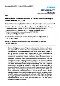
Figure 1. Examples of auroral precipitation energy flux images before (left) and after (right) noise was deleted by image checking for the TIMED/GUVI orbit 7840 around 23:00 UT at day 140, 2003 in the Northern Hemisphere. [8] In this work, GUVI observations from February 2002 to October 2007 were used. During this period, over 55,000 images (28–30 images per day) were available. This large quantity of data has allowed us to unambiguously separate seasonal and hemispheric variations of the precipitation with geomagnetic activity. The energy flux inferred from the FUV data might have uncertainties in some individual images. For weak aurora (Kp = 0, 1), the original emission count rate is low, which may arouse high percentage error. If the original emission data error was 50%, the averages of ∼100 auroral images covering the same MLT sectors would reduce the percentage error to 3% within a grid of 40 × 40 km. In the present study, we use averaged values from a large amount of observational images, which tends to cancel out possible random uncertainties of the FUV technique. 2.2. Further Noise Removing [9] One of the challenges in this study was to further remove the residual, bright dayglow emission under sunlit conditions, especially under geomagnetically quiet conditions, when the noise due to dayglow could cause errors in estimating the total auroral hemispheric power. This noise is significant in most of the originally published GUVI energy flux images during summer daytime, even after the primary dayglow removal procedure described above was applied (see Figure 1, left, for an example). In this work, extra steps were adopted to further reduce this residual dayglow as well as some other random noises. A major procedure was to delete scattered noise points (or “pixels”) by checking images for each orbit. To delete residual dayglow, we assumed that electron precipitation (both weak and intense) occurred continuously in a particular location and then checked each image bin (0.5 h × 1° in MLT and MLAT) to see how much signal occurred in it. If the illuminated points were insufficient (i.e., no larger than ∼44% of the total “pixels” or points in a bin, which is equivalent to a condition of no larger than 4 “pixels” of a total of 9 “pixels” at MLAT 80° and no larger than 14 “pixels” of a total of 33 “pixels” at MLAT 60°), these points were considered as noise and set to
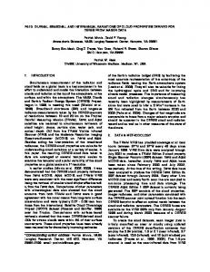
zero. Figure 1 shows an example of auroral precipitation energy flux images before and after noise was deleted by image checking for TIMED/GUVI orbit 7840 around 23:00 UT on day 140, 2003 in the Northern Hemisphere. Most of the scattered noise points outside the auroral illumination region were deleted without losing any information about the auroral precipitation itself. Note that the binned image unit of 0.5 h × 1.0° in MLT and MLAT was small enough to allow even the thinnest part of the auroral oval, just after noon around MLAT 70°, to be completely kept after noise had been deleted (Figure 1). This process removed most of the noise in the auroral region, since the auroral illumination oval was usually a thin and small part of the total auroral region in the daytime sector, as shown in Figure 1. [10] Figure 2a (left) shows comparisons for MLT = 12 and Kp = 1 conditions in the northern summer between the originally derived energy fluxes and those with noise reduced by applying our noise‐deleting procedures. The originally derived energy fluxes here refer to the fluxes from GUVI images published on the Web site. These original images were processed using the primary dayglow emission reduction [Zhang and Paxton, 2008] that was described in section 2.1. From Figure 2a, we see that, when our noise reduction procedure was used, the energy flux was reduced to near zero at MLATs lower than 70°, where no aurora occurred, and that noise in the polar cap was also much reduced. Thus, our noise deletion method was effective. Figure 2a also shows that the baseline noise was estimated to be between 0.1 and 0.2 erg/s/cm2 for MLAT 50°–90°. This baseline was at its largest near the MLT 12 sector but was much reduced in regions away from this sector; it reached a minimum in the nighttime region. Figure 2b gives the absolute differences between Hemispheric Power (HP) calculated using the original data and that calculated with noise deleted (i.e., the hemispherically integrated energy flux induced by noise) in local summers and local winters in both hemispheres. The error in hemispheric power caused by noise was between ∼5–7 GW in summer and ∼2–4 GW in winter in both hemispheres. Note that the noise level was
3 of 15
A11304
LUAN ET AL.: VARIATIONS OF ENERGY FLUX FROM TIMED/GUVI
A11304
Figure 2. Comparison between the originally derived energy flux and those with noise deleted: (a) auroral energy fluxes under conditions of MLT = 12 and Kp = 1 in the northern summer. (b) The absolute differences of hemispheric power (HP) between the originally derived auroral patterns and those with noise being deleted in the summer and winter in both hemispheres, respectively. the same between the Northern and Southern hemispheres in the same season for each Kp level. There was a trend of increasing noise level with increasing Kp indices, which was due to the fact that generally higher geomagnetic activity and stronger solar radiation occurred around solar maximum (2002–2004) than solar minimum (2005–2007), and thus, higher dayglow noise levels occurred under higher Kp conditions. 2.3. Data Bin Method [11] The final, averaged energy flux in each 0.5 h × 0.5° bin after the noise‐deleting procedure was used in our analysis here. To calculate the total hemispheric power, the data were binned into 8 levels of the Kp index from 0 to 7. At each Kp level, the data were binned using three adjacent Kp values. For instance, the Kp 1 level included all data when Kp values were 0.7, 1.0, and 1.3, respectively. Under each Kp level, the hemispheric power (i.e., the total energy flux over the whole auroral oval in one hemisphere) was then calculated by hemispherically integrating the averaged energy flux from each bin according to the area of each bin. In this study the hemispheric power was integrated within the 50°–90° MLAT and 0–24 MLT intervals. Our analysis was carried out in both the June and December solstice seasons in each hemisphere. The June/December solstice seasons included a period of 90 days that was centered at each solstice day to obtain a good MLT and MLAT coverage of the auroral precipitation. [12] Figure 3 illustrates the orbit count number (the number of times the bin was imaged) in each solstice season of both hemispheres for different Kp levels (Kp = 1–5). The orbit counts were mostly more than 400 for Kp = 1–3 and above 200 for Kp = 4 and above 100 for Kp = 5. The orbit counts in most auroral regions were only about 25 for Kp = 6 and about 5 for Kp = 7 (not shown here). The uneven orbit counts during magnetic daytime and nighttime in each season were caused by the orbit position of the TIMED
satellite. Because of small HP for Kp = 0 and low observational sample counts for high Kp (Kp = 6, 7), we have concentrated on conditions from Kp 1 to 5 in the present work.
3. Results [13] In this section we calculate the hemispheric power from the averaged pattern of the auroral energy flux (section 3.1) and quantitatively compare the hemispheric power under three conditions: (1) between the local summers (winters) of the two hemispheres (section 3.2), (2) in each hemisphere between the summer and winter seasons (section 3.3), (3) interhemispherically around each solstice period between the Northern and Southern hemispheres (section 3.4). In addition, the winter‐summer difference is also compared for different MLT regions (section 3.5). When the patterns of both the absolute and percentage difference are considered, we refer to their absolute values regardless of their sign, if not otherwise specified. 3.1. Hemispheric Power and Standard Deviations [14] Figure 4 gives the averaged patterns of the auroral energy flux in magnetic latitude and local time coordinates, corresponding to each condition in Figure 3. These statistical patterns of auroral energy flux showed all the locations where precipitation could occur, whereas the real auroral oval would move within locations shown by the averaged values. Higher averaged precipitation energy flux occurred at locations where there was either more intense precipitation or a higher occurrence frequency of precipitation or both. Note that the units of ergs/s/cm2 that we used in this study are the same as mW/m2. The hemispheric power under each condition is listed in Table 1a, varying between 2.4 and 172.5 GW for Kp values from 0 to 7. HP increased greatly with the Kp index in all the solstice seasons and both hemispheres from Kp 1 to 5. As shown in Table 1a, HP varied from 9.2 to 66.6 GW in the
4 of 15
A11304
LUAN ET AL.: VARIATIONS OF ENERGY FLUX FROM TIMED/GUVI
A11304
Figure 3. The observational orbit counts under different Kp conditions (Kp = 1–5) in the June solstice and December solstice in both the Northern (left two) and Southern (right two) hemispheres. northern summer and from 10.9 to 67.9 GW in the southern summer. Similarly, in winter, HP varied from 8.1 to 65.0 GW in the Northern Hemisphere and from 7.7 to 68.9 GW in the Southern Hemisphere. [15] The hemispheric power (HP), calculated from the averaged pattern of Figure 4, represented the averaged total energy flux in each season over each hemisphere. A direct calculation of variations of HP for each Kp level is not available, since under real conditions the precipitation occurs only in part of the total averaged oval in Figure 4. To estimate the standard deviation of the hemispheric power, we did a statistical study of the hemispheric power for all days from 2002 to 2007. In each case, the auroral ovals were completed by images from both the northern and southern hemispheric observations under each Kp level within 3 h. Therefore, in each case, one auroral oval included 2–4 superposed images since the TIMED/GUVI orbit period is about 1.5 h. Figure 5 shows statistical results of this superposition, including (a) an example of a completed auroral oval from images observed from both hemispheres in Kp 3 conditions (Kp = 2.7) within 5.7–8.2 UT hours on day 72, 2003;
(b) the averaged hemispheric power with standard deviations under Kp 1–5 conditions; and (c) the corresponding case counts. For Kp 1–5, the averaged HP was 8.3, 17.9, 29.4, 46.4, and 67.6 GW, with standard deviations (sHP) of 4.2, 6.8, 9.1, 13.0, and 18.2 GW, respectively. Note that the averaged HP from individual cases was in very good agreement with that from the binned data (see Table 1a) at each Kp level, which indicates that the averaged HP integrated from averaged energy flux in individual bins is equivalent to that from global auroral oval. [16] The large variations of HP come mainly from large variations of brightness due to precipitation in each MLT sector as well as the variations of locations where the precipitation occurs. In the present study, additional large fluctuations of HP were produced by variations of geomagnetic activity for each Kp level as well as the coarse time resolution of the Kp index. Because of a close correlation between the hemispheric power and the Kp index, the hemispheric power fluctuated with small changes in the Kp indices in each Kp level, especially at high Kp levels. Under Kp 1–5 conditions, the standard deviation of the Kp indices
5 of 15
A11304
A11304
LUAN ET AL.: VARIATIONS OF ENERGY FLUX FROM TIMED/GUVI
Figure 4. Averaged electron energy fluxes at different Kp levels in each solstice season of both the northern (two left frames) and southern (two right frames) hemispheres. at each Kp level varied between 0.2 and 0.25, which caused corresponding HP deviations of 2.0–5.8 GW from Kp 1 to 5. However, these variations due to geomagnetic activity would not affect the averaged value of HP, since the averaged Kp indices in all seasons/hemispheres were balanced for each Kp level when Kp was less than 5, as shown in Table 1b. For Kp 5, there was a slightly higher averaged Kp index (by ∼0.08) in the June solstices than in the December solstices. Other HP variations are expected due to the coarse time resolution of the Kp index. It was possible that the Kp index might not reflect the actual geomagnetic activity for some images. This source of fluctuations of HP should occur randomly, and thus would not affect the averaged values of HP for each Kp level when there were sufficient observational samples, especially for Kp 1–4. We have tested that the magnitude of HP and the standard deviations of HP from the case study changed little (mostly ≤ 0.7 GW for HP and ≤ 0.3 GW for sHP) from the value we listed in the above during either the solstice or equinoctial period and also during different parts of the solar cycle (2002–2004 as opposed to 2005–2007). Further, as we will discuss in
section 4.1, there were generally persistent seasonal/hemispheric variations in HP, although the absolute magnitude of the seasonal/hemispheric asymmetry in HP was smaller than the standard deviation of HP at each Kp level. 3.2. Hemispheric Differences in Each Season [17] The top frames in Figure 6 show the absolute and percentage hemispheric power (HP) differences (northern minus southern HP) between the northern summer (June solstice) and southern summer (December solstice), whereas Table 1a. Hemispheric Power in June and December Solstice Seasons in Both the Northern and Southern Hemispheres for Kp 0–7a Season/Kp
0
1
2
3
4
5
6
7
Jun/NH (summer) Dec/NH (winter) Jun/SH (winter) Dec/SH (summer)
3.6 3.0 2.4 4.8
9.2 8.1 7.7 10.9
18.4 17.2 17.7 20.0
30.2 28.8 29.2 30.5
46.1 46.9 46.1 44.8
66.6 65.0 68.9 67.9
84.2 97.5 87.9 97.8
137.0 172.5 147.1 150.8
6 of 15
a
Units are in GW.
A11304
A11304
LUAN ET AL.: VARIATIONS OF ENERGY FLUX FROM TIMED/GUVI
Figure 5. An estimate of the standard deviations of the hemispheric power from case study: (a) an example of a completed auroral oval image observed from both hemispheres under similar Kp conditions within 3 h on day 72, 2003; (b) the averaged hemispheric power with standard deviations; and (c) the corresponding case counts under different Kp conditions. the bottom frames give the differences for the winter seasons. The percentage difference was the ratio of the absolute difference between the Northern and Southern Hemisphere to the averaged HP over both hemispheres. The same methods have been applied to other similar comparisons in this study. The right frames in Figure 6 show that, in winter, there were nearly no percentage differences between the two hemispheres from Kp 1 to 5. The absolute differences between the two winters were near zero for Kp ≤ 3, 0.8 GW for Kp 4, and 3.9 GW for Kp 5, whereas these differences in HP were negligible at higher Kp. In summer the HP in the Southern Hemisphere was larger by 1.6–1.7 GW than its Northern Hemisphere counterpart for Kp lower than 3. The percentage difference was about 20% for Kp = 1 and 10% for Kp = 2. However, the absolute differences of 1.3 GW between the two summers under Kp 4–5 conditions were negligible relative to the HP under these same conditions. Therefore, there were no clear HP differences between the two summer hemispheres from Kp 3 to 5. The percentage differences of Hp between the hemispheres in summer decreased with increases of the Kp index and hence geomagnetic activity. 3.3. Seasonal Variations in Each Hemisphere [18] Figure 7 shows the differences of the hemispheric power between the June and December solstices in the Northern and Southern hemispheres, respectively. In each hemisphere, the HP was higher by 1.1–3.2 GW in summer than in winter for geomagnetically undisturbed conditions (Kp ≤ 3), whereas there was no clear difference for moderately disturbed conditions (Kp = 4 and 5) relative to the HP in the same conditions. For Kp from 1 to 3, the percentage difference decreased
from about 13% to 5% in the northern hemisphere, and from about 35% to 4% in the Southern Hemisphere. The percentage difference in the Southern Hemisphere was 22% higher than that in the Northern Hemisphere at Kp = 1 but only 5% higher at Kp = 2. Thus, the summer‐winter asymmetry was larger in percentage in the Southern Hemisphere than in the Northern Hemisphere for low Kp conditions. Note that similar magnitudes of summer‐winter differences in HP occurred under Kp 4 and 5 as those under Kp ≤ 3 conditions in both hemispheres, but the large HP under higher Kp conditions ensured that there were no apparent percentage differences. 3.4. Seasonal/Hemispheric Variation Between the Two Hemispheres [19] Figure 8 gives both the absolute and percentage differences of hemispheric power between the Northern and Southern hemispheres in the same period (e.g., either June solstice or December solstice, northern minus southern HP). Similar to the seasonal variations in one hemisphere, HP in the same solstice period had obviously higher values in the summer hemisphere under geomagnetically quiet conditions Table 1b. Averaged Kp Index in June and December Solstice Seasons in Both the Northern and Southern Hemispheres for Kp 0–7 Conditions Season/Kp
0
1
2
3
4
5
6
7
Jun/NH (summer) Dec/NH (winter) Jun/SH (winter) Dec/SH (summer)
0.25 0.14 0.25 0.14
1.00 0.98 1.00 0.98
1.99 2.01 2.00 2.01
2.97 3.00 2.97 3.00
3.94 3.96 3.95 3.95
4.98 4.91 4.99 4.90
5.91 5.91 5.91 5.90
7.00 6.88 7.05 6.92
7 of 15
A11304
LUAN ET AL.: VARIATIONS OF ENERGY FLUX FROM TIMED/GUVI
A11304
Figure 6. Differences of hemispheric Power between the Northern and Southern hemispheres in each solstice season. (left) the absolute hemisphere power differences and (right) the percentage differences. (Kp ≤ 3), whereas no clear trend occurred for geomagnetically disturbed conditions when the HP was high. For Kp ≤ 3, the hemispheric differences were between 0.7 and 1.5 GW in June and between 1.7 and 2.8 GW in December. As Kp increased from 1 to 3, the percentage difference decreased from 20% to 4% for the June solstice, whereas it was reduced from about 30% to 5% for the December solstice. Thus, for all Kp levels from 1 to 3, the percentage difference between the two hemispheres in the December solstice was higher than that in the June solstice. For instance, the percentage
difference was about 12% higher in the December solstice than in the June solstice for Kp = 1 and about 10.5% higher for Kp = 2, which was consistent with the results in section 3.2 that showed the hemisphere power was greater in the southern summer than in the northern summer. 3.5. Summer‐Winter Difference in Different MLT Sectors [20] Figure 9 shows the absolute and percentage differences of the area‐integrated energy flux (part of the hemi-
Figure 7. Hemispheric power differences June minus December solstice between June and December solstices in each hemisphere. (left) Absolute hemisphere power differences and (right) percentage differences. 8 of 15
A11304
LUAN ET AL.: VARIATIONS OF ENERGY FLUX FROM TIMED/GUVI
A11304
Figure 8. Differences of hemispheric power Northern minus Southern between Northern and Southern hemispheres in the same period (e.g., June solstice and December solstice). (left) Absolute hemisphere power differences and (right) percentage differences.
spheric power) between the winter and summer in the Northern Hemisphere in different MLT sectors for Kp levels from 1 to 5. The results are presented in sectors of premidnight (2000–0000 MLT), postmidnight (0000–0400 MLT), morning/dawn (0400–0800 MLT), daytime (0900–1500 MLT), and evening/dusk (1600–2000 MLT), respectively. [21] In Figure 9, the most prominent feature was the generally higher energy flux in winter than in summer for most Kp levels in the MLT 2000–0000 sector, where most of the discrete aurorae occur. This result is consistent with previous studies, which showed that the discrete aurorae were suppressed by solar EUV radiation under summer/ sunlight conditions [Newell et al., 1996, 1998; Liou et al., 1997, 2001; Hamrin et al., 2000, 2005; Lyatsky et al., 2001; Shue et al., 2001]. From Figure 9, there is a generally increasing winter‐summer asymmetry with the Kp index in the 2000–0000 MLT sector when Kp was less than 5. This result is also consistent with the results of Shue et al. [2001], which showed that there was an anticorrelation between the solar produced ionospheric conductivity and the auroral brightness at 23 MLT and 65° MLAT. In this sector, they reported that the auroral brightness was stronger under southward IMF Bz conditions than under all Bz conditions. In both the daytime (0900–1500 MLT) and dusk (1600– 2000 MLT) sectors, there was a constantly higher integrated energy flux in the summer than in the winter from Kp 1 to 5, whereas there were only significant percentage differences between summer and winter for lower Kp conditions. The solar illumination effect during daytime was generally consistent with the observation from Polar UVI [Liou et al., 1997, 2001]. Both their and our observations showed afternoon (∼1500 MLT) hot spots under summer/sunlit
conditions; but these hot spots did not occur under winter/ dark conditions (Figure 4). [22] In Figure 9, the results show no clear trend for summer‐winter asymmetry with increases of Kp in the morning/dawn (0400–0800 MLT) sector. The bright auroral emissions from midnight to the morning side in both the winter and summer (Figure 4) suggest that TIMED/GUVI captured the features associated with hard electron auroral precipitation. This hard precipitation has been detected by X‐ray observations on the POLAR satellite [Anderson et al., 2000; Petrinec et al, 2000] and also DMSP observations [Newell et al., 2009] from the late evening to the late morning hours (2100−0900 MLT). Newell et al. [2009] suggested that this stronger diffuse precipitation is caused by electrons from the nightside plasma sheet that convect eastward because of the E × B drift. The ion aurora that was seen in TIMED/GUVI observations [Zhang and Paxton, 2008] might also contribute to the bright winter emissions there, since, in the MLT hours from midnight to dawn, the ion precipitating energy flux was about 15%–40% higher in winter than in summer [Newell et al., 2005]. [23] The winter‐summer difference in the Southern Hemisphere was similar to that in the Northern Hemisphere for the above discussed MLT sectors (not presented here), except that the values of absolute differences were larger for the daytime (0900–1500 MLT), morning/dawn (0400– 0800 MLT), and evening/dusk (1600–2000 MLT) sectors. This increased difference was due to larger summer precipitation in the Southern Hemisphere than in the Northern Hemisphere. Hence, the percentage difference in these sectors was much larger in the Southern Hemisphere than in the Northern Hemisphere for lower Kp conditions (Kp ≤ 3).
9 of 15
A11304
LUAN ET AL.: VARIATIONS OF ENERGY FLUX FROM TIMED/GUVI
A11304
Figure 9. The (left) absolute and (right) percentage differences of the hemispheric power (HP) between winter and summer in the Northern Hemisphere in different MLT sectors from Kp 1 to 5. From the top to bottom, it shows the results during premidnight (2000–0000 MLT), postmidnight (0000–4000 MLT), daytime (9000–1500 MLT), morning/dawn (4000–8000 MLT), and evening/dusk (1600–2000 MLT) hours, respectively.
3.6. Contributions of Energy Fluxes From Different Sectors to the Total Hemispheric Power [24] Figure 10 shows the percentage ratio of the integrated energy flux in the nighttime (2100−0300 MLT) and daytime (0900–1500 MLT) sectors to the total hemispheric power at different Kp levels for different seasons in each hemisphere. In winter, the results show nearly constant percentage ratios in both the daytime (∼5%) and nighttime (∼50%) sectors in each hemisphere for all Kp levels. In summer, the percentage ratio increased during nighttime and decreased during daytime with increasing Kp to near the constant levels that occurred in winter, thus at higher Kp (≥4) values, the percentage contribution of the energy flux in the same sector became similar in different seasons and hemispheres, which was consistent with the disappearance of the seasonal and hemispheric differences of HP shown earlier (Figures 5–7). At higher Kp values, roughly the same energy percentage
occurred for all seasons and hemispheres in each sector, which indicated that there was little or no effect of solar illumination on the seasonal and hemispheric differences of HP. It also suggested that the auroral precipitation energy flux increased with Kp in similar ways for different MLT sectors from low to higher Kp levels in winter.
4. Discussion 4.1. Extent of Summer‐Winter Difference [25] The results from Figures 6–8 show absolute differences of about 1–3 GW between the summer and winter seasons or hemispheres and also differences of about 2 GW between northern and southern summers under low geomagnetic activity conditions. These differences were smaller than the magnitudes of the estimated standard deviations of HP under each Kp level of 1–3. However, for these low Kp
10 of 15
A11304
LUAN ET AL.: VARIATIONS OF ENERGY FLUX FROM TIMED/GUVI
Figure 10. The percentage of the integrated energy flux in the nighttime (2100−0300 MLT) and daytime (0900– 1500 MLT) regions to the total hemispheric power under different Kp levels in each season and hemisphere. conditions, the imaging times in all the auroral oval regions were above 400; thus, the averaged HP would not be affected by the large deviations of HP. More important, the magnitude and trend of the summer‐winter differences were persistent for all different conditions of Kp 1–3 (Figures 7–8); thus, they were not affected by the relatively large random variations of HP due to the coarse time resolution of the Kp index. Further, as we mentioned in section 3.1, the averaged HP and its standard deviations remain constant when the observational samples are large enough. For similar reasons, the small differences between the two summers under Kp < 3 were also real. Because of the low background HP during geomagnetically quiet conditions, the differences in HP between the summers of the two hemispheres resulted in percentage differences of 10%–20% for Kp 1–2, and the differences between summer and winter seasons or hemispheres resulted in percentage differences of 4%–35% for Kp 1–3. The above percentage differences decreased with increasing Kp. The magnitude and trend of the summer‐ winter differences when Kp was 4 were also persistent from Figures 7–8. When Kp was 4, the absolute HP was slightly larger in winter than in summer, suggesting a reversal of the summer‐winter difference trend from geomagnetically quiet to moderately disturbed conditions. Note that the summer‐ winter trend in absolute differences of HP when Kp was 5 was random for different comparisons in Figures 7–8, which suggested that the averaged HP when Kp was 5 may have been affected by the relatively small sample size. When Kp was 5, the winter HP in the northern hemispheres may have been underestimated in comparison with the absolute variation trend of Kp 4 (Figures 6–9). However, the effects of relatively fewer samples when Kp was 5 should not have been significant, since the percentage differences were similar between Kp 4 and 5 conditions for all of the comparisons in Figures 6–8. Overall, there were no significant absolute summer‐winter differences in auroral hemispheric power for Kp 4–5 conditions, whereas TIMED/
A11304
GUVI observations showed persistent summer‐winter differences in magnetically quiet conditions, although in absolute terms these represent relatively small changes in HP. [26] Our results for the summer‐winter difference of hemispheric power were similar to those of Liou et al. [2001] for geomagnetically quiet conditions, when the larger daytime precipitation energy fluxes in the summer were considered. During 2000−0000 MLT, the winter‐summer asymmetry in the integrated energy flux was 3%–10% for Kp 1–4 conditions (Figure 9). The results of Liou et al. [2001] showed that the winter‐to‐summer ratio of the energy flux was 5 ergs/s/cm2, defined by Newell et al. [1996]) occurring in winter was only ∼6% according to observations from DMSP satellites during 1984–1992. This probability was calculated by dividing the number of spectra taken in a bin that showed signs of electron acceleration by the total number of spectra taken in that bin. In fact, a recent study using DMSP observations over one solar cycle showed that the diffuse auroral energy flux made up 71%–84% of the total precipitation energy budget under both low and active solar wind driving conditions [Newell et al., 2009]. Therefore, for both geomagnetic quiet and disturbed conditions, the much larger proportion of diffuse auroral energy flux in the total precipitation power limits the extent of winter‐summer differences in hemispheric power caused by the discrete auroral precipitation. [29] Under geomagnetically disturbed conditions, our results did not show the significant winter‐summer asymmetry of 20%–40% in hemispheric power that was seen in NOAA and DMSP satellites observations [Emery et al., 2008]. This significant asymmetry, with higher hemispheric power in winter than in summer, should require much larger winter‐summer asymmetry ratios in the nighttime sector [Emery et al., 2008], which is not supported by the present study and some previous work [Liou et al., 1997, 2001; Newell et al., 2009]. Our results did show that the precipitation energy flux was higher in winter than in summer in both the premidnight and postmidnight sectors, where the precipitation was mostly attributed to diffuse aurorae [Newell et al., 2009]. However, this nighttime winter‐
11 of 15
A11304
LUAN ET AL.: VARIATIONS OF ENERGY FLUX FROM TIMED/GUVI
summer asymmetry was no higher than 10% (Figure 9). There have been observations that exhibited higher occurrence frequency of diffuse aurora during magnetic nighttime in darkness compared to sunlight [Hamrin et al., 2005], whereas there were some suggestions of higher electron precipitation in summer than in winter in the late morning sector because of the increased regions 1 and 2 currents in sunlight [Liou et al., 1997, 2001; Shue et al., 2001]. 4.2. Cause of Summer‐Winter Differences Under Low Kp Conditions [30] Although the mechanisms causing the summer‐winter difference of the discrete aurora are still under debate, the suppressing effect of solar illumination on relatively intense auroral precipitation during premidnight has been reported in various studies [e.g., Newell et al., 1996, 1998, and 2001; Liou et al., 1997, 2001; Lyatsky et al., 2001; Ohtani et al., 2009]. Our results show different solar illumination effects on the auroral precipitation energy flux, not only between magnetic daytime and night time but also between different Kp levels. Because there were no obvious hemispheric differences under dark conditions, the summer‐winter difference of the HP for lower Kp values can be largely attributed to the effects of solar illumination. The effect of solar illumination on auroral precipitation can be related to its effect on the conductance and the resultant currents and electron acceleration because the photoelectrons that contribute to the ionospheric conductivity are controlled by solar EUV radiation. Solar‐driven ionospheric conductance changes as a function of solar zenith angle and the solar EUV flux [Rasmussen et al., 1988]; hence, the ionospheric conductance is dramatically changed from summer to winter. Under lower geomagnetic activity conditions, the solar radiation induced conductance is the dominant part of total ionospheric conductance at high latitudes; thus, the intensity of the solar illumination has a significant effect on the total precipitation energy flux. Hardy et al. [1987] estimated that, at high latitudes in summer, the ratio of aurora‐produced, height‐integrated Pedersen conductivity to that of the solar‐ produced conductivity varies diurnally between 0.4 and 0.49 at local noon when Kp = 2; the ratio becomes larger around the winter solstice. [31] There are a few additional processes that can lead to the differences in the solar‐EUV produced conductivity between the northern and southern hemispheres besides seasonal effects. The most important fact is that the southern magnetic pole lies at a lower geographic latitude than the northern pole does because of the eccentricity of the dipole, resulting in larger diurnal variations of the solar zenith angle and greater ionospheric conductance on average in the southern auroral oval region [Hurtaud et al., 2007]. In addition, the magnetic field strength is stronger at the northern magnetic pole than that at the southern pole, resulting in a larger conductance in the Southern Hemisphere for comparable solar zenith angles [Hurtaud et al., 2007]. Also, the differences in HP between summers in the northern and southern hemispheres may have additional contributions from the change of the Sun‐Earth distance. There is a 3% variation in Sun‐Earth distance between January and July, which leads to about 7% more solar radiation flux being received by the Earth in the December solstice than in the June solstice.
A11304
[32] Auroral activity responds to solar illumination in different ways between magnetic daytime and nighttime. The solar illumination effect on the auroral precipitation energy flux can be further demonstrated by the averaged area‐integrated energy flux binned by universal time. Figure 11 gives an example of this flux for Kp = 2 in both hemispheres (NH and SH) in the solstice season for the daytime sector (0900–1500 MLT) and for the discrete aurora region at night (2100–0100 MLT). Results in summer and winter in both hemispheres are presented. In the daytime, larger energy fluxes occurred in summer than in winter in both hemispheres, whereas, at night, larger overall energy fluxes occurred in winter in both hemispheres. Note that the precipitation energy flux was larger in the southern December/summer than in northern June/summer during most of the day due to the greater background solar illumination. However, for lower Kp indices, the magnitude of the integrated energy flux of summer exceeding that in winter in the magnetic daytime and dusk sectors, outweighed that of winter exceeding summer in the magnetic nighttime sector (Figures 9 and 11). This resulted in greater net hemispheric power in the summer season/hemisphere than in the winter season/hemisphere. [33] Results from Liou et al. [2001] using POLAR/UVI showed that the number flux of auroral precipitation was lower in the dark hemisphere than in the sunlit hemisphere for all MLT regions. They suggested that the increase of dayside auroral power in summer might be associated with the large‐ scale upward field‐aligned currents, which peak in summer, as well as large increases in the electron number flux. The suppression of the nightside auroral power in summer was also associated with a large decrease in the electron energy. There have been many studies that discuss the ionospheric feedback with relatively intense auroral precipitation under dark (winter) conditions, when the solar‐produced conductivity and electron density are low [e.g., Newell et al., 1996, 1998, and 2001; Liou et al., 1997, 2001; Lyatsky et al., 2001; Ohtani et al., 2009]. The energy flux in both the noon time and discrete aurora sectors showed obvious UT time variations, which is of interest for future work. 4.3. Why Does Summer‐Winter Difference Disappear Under Higher Kp Conditions [34] Our results showed that the seasonal and hemispheric differences in total hemispheric power, which are associated with different solar illumination conditions when Kp ≤ 3, disappeared when the Kp index was larger than 3. This result is in contrast to the significant seasonal asymmetry derived from NOAA and DMSP satellites observation [Emery et al., 2008]. The disappearing of the seasonal and hemispheric differences at higher Kp levels can be explained by the stronger auroral precipitation energy flux at these higher Kp levels, in addition to the dominant contribution of the diffuse aurora to the hemispheric power under active solar wind driving conditions [Newell et al., 2009]. First, the total hemispheric power increased greatly and nonlinearly with Kp as Kp became larger than 3, as shown in Table 1a. This increase of hemispheric power would increase the proportion of auroral‐induced ionospheric conductance and decrease the relative role of the solar EUV produced conductance. As assumed by Hardy et al. [1987] and Hurtaud et al. [2007], the integrated Pedersen conductivity was proportional to the square root of the hemispheric power.
12 of 15
A11304
LUAN ET AL.: VARIATIONS OF ENERGY FLUX FROM TIMED/GUVI
A11304
Figure 11. Diurnal variations of the averaged area integrated energy fluxes under Kp = 2 condition in both hemispheres (NH and SH) in solstice seasons: (a) during the daytime sector (0900–1500 MLT) and (b) for discrete aurora region (2100–0100 MLT). Figures 6–7 suggest that there was a change in the trend of the absolute winter‐summer differences in hemispheric power for low (≤3) to higher (= 4) Kp indices. Second, the sharply increased hemispheric power at higher Kp values would decrease the percentage difference between summer and winter if the absolute difference in hemispheric power between summer and winter was the same at high Kp as it was at low Kp. In Figure 9, the absolute difference of integrated energy flux between the summer and winter hemisphere remained about the same level for Kp 1–5 on the daytime and dusk sides of the auroral oval, whereas the percentage difference decreased with increasing Kp index. Figure 10 shows that, when Kp values were higher than 3, the auroral precipitation contributed at roughly the same ratio to the total HP for all seasons in each sector of the daytime (9–15 MLT) and the nighttime (21−03 MLT), which indicated that the relative difference in the hemispheric power between summer and winter and between summers in Northern and also Southern hemispheres disappeared. [35] It is worth noting that, although the averaged total energy deposited in both hemispheres due to auroral precipitation was the same under geomagnetically disturbed conditions, the time evolution and geographic distribution of the auroral precipitation energy flux could be different between two hemispheres [Sato et al., 1998; Østgaard et al., 2003 and 2004; Stubbs et al., 2005]. Our results at each Kp level were averaged over all UT times and integrated from the entire auroral oval from MLAT 50–90 and MLT 0–24 in each hemisphere; thus, they smoothed out UT effects and possible effects due to different geomagnetic morphologies in the two hemispheres.
4.4. Seasonal Variations of the Hemispheric Power and Geomagnetic Activity [36] The GUVI results showed that, when Kp was higher than 3, the seasonal/hemispheric variations of the hemispheric power disappeared. However, since there was a high correlation between geomagnetic activity and hemispheric power because of their same origin in the solar wind/IMF [Emery et al., 2009; Luan et al., 2009], any seasonal variations of geomagnetic activity should be accompanied by similar variations in the hemispheric power. As shown in Table 1a, the amount of increase in the hemispheric power with Kp index was much larger than the amount of difference between the summer and winter seasons even under low Kp index conditions. The GUVI observations were conducted during the declining phase of solar cycle 23, when the geomagnetic activity was generally higher in the December solstice than in the June solstice and the seasonal variation of the hemispheric power had the same trend [Luan et al., 2009]. Therefore, it is important to examine the seasonal/hemispheric variations of the hemispheric power under the same geomagnetic activity conditions and to study how variations in seasonal and hemispheric asymmetries changed with changing geomagnetic activity.
5. Summary and Conclusions [37] Using TIMED/GUVI observations during 2002– 2007, the seasonal variations in the auroral hemispheric power (HP) have been separated from hemispheric and geomagnetic activity dependencies. For each of the geomagnetic activity levels of Kp 1–5, the seasonal and hemispheric variations of the auroral hemispheric power have
13 of 15
A11304
LUAN ET AL.: VARIATIONS OF ENERGY FLUX FROM TIMED/GUVI
been investigated. The main points of the present work can be summarized as: [38] 1. There were almost no hemispheric differences in HP between the local winters of both hemispheres under similar geomagnetic activity conditions. [39] 2. Under geomagnetically quiet conditions, the hemispheric power showed summer‐winter differences in each hemisphere and interhemispherically and also showed northern summer (June solstice) to southern summer (December solstice) differences. Under these conditions, the hemispheric power was higher in the summer season/ hemisphere than in the winter season/hemisphere and higher in the southern summer than in the northern summer. [40] 3. The relative differences between two local summers and between the summer and winter season/hemisphere were within the order of 0%–35% for Kp 1–3; these differences decreased with increasing Kp indices. These seasonal/ hemispheric variations in the hemispheric power disappeared during geomagnetically disturbed conditions (Kp = 4 and 5). [41] 4. Under lower Kp conditions (≤3), the differences of hemispheric power between summer and winter and between local summers in the two hemispheres were probably caused by different solar illumination conditions. For Kp ≤ 3, although larger precipitation energy flux was favored under winter/dark conditions in the nighttime discrete aurora sector, much larger energy fluxes were associated with solar illumination/sunlit in summer for daytime MLT sectors. [42] 5. Our results also showed that the amount of increase in the hemispheric power with the Kp index was much larger than the differences between the summer and winter seasons even under low Kp conditions. [43] Acknowledgments. We are grateful for discussion with Art Richmond and Barbara Emery in HAO, NCAR. This research is supported by NASA grants NNH08AH37I, NNX08AQ91G, and NNX09AI04G, and in part by the Center for Integrated Space Weather Modeling (CISM) which is funded by the STC program under agreement ATM‐0120950. The National Center for Atmospheric Research is sponsored by the NSF. The GUVI data used here are provided through support from the NASA MO&DA program. [44] Robert Lysak thanks the reviewers for their assistance in evaluating this paper.
References Anderson, P. C., D. L. McKenzie, M. J. Brittnacher, M. W. Chen, M. Hairston, and M. F. Thomsen (2000), Global storm time auroral X‐ray morphology and timing and comparison with UV measurements, J. Geophys. Res., 105(A7), 15,757–15,777, doi:10.1029/1999JA000355. Barth, C. A., D. N. Baker, and S. M. Bailey (2004), Seasonal variation of auroral electron precipitation, Geophys. Res. Lett., 31, L04809, doi:10.1029/2003GL018892. Christensen, A. B., et al. (2003), Initial observations with the Global Ultraviolet Imager (GUVI) in the NASA TIMED satellite mission, J. Geophys. Res., 108(A12), 1451, doi:10.1029/2003JA009918. Daniell, R. E., Jr. (1993), Modeling of optical signatures of electron spectra in the ionospheric heating experiments, in Proceedings and Program for the Seventh International Ionospheric Effects Symposium, p. 6B/5/1, SRI‐Int, Arlington, Va, USA. Emery, B. A., V. Coumans, D. S. Evans, G. A. Germany, M. S. Greer, E. Holeman, K. Kadinsky‐Cade, F. J. Rich, and W. Xu (2008), Seasonal, Kp, solar wind, and solar flux variations in long‐term single‐pass satellite estimates of electron and ion auroral hemispheric power, J. Geophys. Res., 113, A06311, doi:10.1029/2007JA012866. Emery, B. A., I. G. Richardson, D. S. Evans, and F. J. Rich (2009), Solar wind structure sources and periodicities of auroral electron power over three solar cycles, J. Atmos. Terr. Phys., 71(10/11), 1157, doi:10.1016/ j.jastp.2008.08.005.
A11304
Hamrin, M., M. André, P. Norqvist, and K. Rönnmark (2000), The importance of a dark ionosphere for ion heating and auroral arc formation, Geophys. Res. Lett., 27(11), 1635–1638. Hamrin, M., P. Norqvist, K. Rönnmark, and D. Fellgård (2005), The importance of solar illumination for discrete and diffuse aurora, Ann. Geophys., 23, 3481–3486. Hardy, D. A., M. S. Gussenhoven, R. Raistrick, and W. J. McNeil (1987), Statistical and functional representations of the pattern of auroral energy flux, number flux, and conductivity, J. Geophys. Res., 92(A11), 12,275–12,294, doi:10.1029/JA092iA11p12275. Hurtaud, Y., C. Peymirat, and A. D. Richmond (2007), Modeling seasonal and diurnal effects on ionospheric conductances, region‐2 currents, and plasma convection in the inner magnetosphere, J. Geophys. Res., 112, A09217, doi:10.1029/2007JA012257. Liou, K., P. T. Newell, C.‐I. Meng, M. Brittnacher, and G. Parks (1997), Synoptic auroral distribution: A survey using Polar ultraviolet imagery, J. Geophys. Res., 102(A12), 27,197–27,205, doi:10.1029/97JA02638. Liou, K., P. T. Newell, C.‐I. Meng, M. Brittnacher, and G. Parks (1998), Characteristics of the solar wind controlled auroral emissions, J. Geophys. Res., 103(A8), 17,543–17,557, doi:10.1029/98JA01388. Liou, K., P. T. Newell, and C.‐I. Meng (2001), Seasonal effects on auroral particle acceleration and precipitation, J. Geophys. Res., 106(A4), 5531–5542, doi:10.1029/1999JA000391. Liu, X.‐C., G.‐X. Chen, W.‐Y. Xu, A.‐M. Du, Y.‐Y. Wu, B. Chen, Y. Wang, and X.‐D. Zhao (2008), Relationships of the auroral precipitating particle power with AE and Dst indices, Chinese J. Geophys., 51(4), 686–693. Luan, X., W. Wang, A. G. Burns, S. C. Solomon, Y. Zhang, and L. J. Paxton (2009), Unusual declining phase of solar cycle 23: Weak semiannual variations of auroral hemispheric power and geomagnetic activity, Geophys. Res. Lett., 36, L22102, doi:10.1029/2009GL040825. Lyatsky, R. L., P. T. Newell, and A. Hamza (2001), Solar illumination as cause of the equinoctial preference for geomagnetic activity, Geophys. Res. Lett., 28(12), 2353–2356, doi:10.1029/2000GL012803. Newell, P. T., C.‐I. Meng, and K. M. Lyons (1996), Suppression of discrete aurorae by sunlight, Nature, 381, 766–767. Newell, P. T., C.‐I. Meng, and S. Wing (1998), Relation to solar activity of intense aurorae in sunlight and darkness, Nature, 393, 342–344. Newell, P. T., R. A. Greenwald, and J. M. Ruohoniemi (2001), The role of the ionosphere in aurora and space weather, Rev. Geophys., 39(2), 137–149. Newell, P. T., S. Wing, T. Sotirelis, and C.‐I. Meng (2005), Ion aurora and its seasonal variations, J. Geophys. Res., 110, A01215, doi:10.1029/ 2004JA010743. Newell, P. T., T. Sotirelis, and S. Wing (2009), Diffuse, monoenergetic, and broadband aurora: The global precipitation budget, J. Geophys. Res., 114, A09207, doi:10.1029/2009JA014326. Ohtani, S., S. Wing, G. Ueno, and T. Higuchi (2009), Dependence of premidnight field‐aligned currents and particle precipitation on solar illumination, J. Geophys. Res., 114, A12205, doi:10.1029/2009JA014115. Østgaard, N., S. B. Mende, H. U. Frey, L. A. Frank, and J. B. Sigwarth (2003), Observations of non‐conjugate theta aurora, Geophys. Res. Lett., 30(21), 2125, doi:10.1029/2003GL017914. Østgaard, N., S. B. Mende, H. U. Frey, T. J. Immel, L. A. Frank, J. B. Sigwarth, and T. J. Stubbs (2004), Interplanetary magnetic field control of the location of substorm onset and auroral features in the conjugate hemispheres, J. Geophys. Res., 109, A07204, doi:10.1029/2003JA010370. Paxton, L. J., D. Morrison, and D. J. Strickland et al. (2003), The use of far ultraviolet remote sensing to monitor space weather, Adv. Space Res., 31(I4), 813–818. Petrinec, S. W., L. Imhof, D. L. Chenette, and J. Mobilia, and T. J. Rosenberg (2000), Dayside/nightside auroral X‐ray emission differences—Implications for ionospheric conductance, Geophys. Res. Lett., 27(20), 3277–3279, doi:10.1029/2000GL000056. Rasmussen, C. E., R. W. Schunk, and V. B. Wickwar (1988), A photochemical equilibrium model for ionospheric conductivity, J. Geophys. Res., 93(A9), 9831–9840, doi:10.1029/JA093iA09p09831. Sato, N., T. Nagaoka, K. Hashimoto, and T. Saemundsson (1998), Conjudacy of isolated auroral arcs and nonconjugate auroral breakups, J. Geophys. Res., 103(A6), 11,641–11,652, doi:10.1029/98JA00461. Shue, J.‐H., P. T. Newell, K. Liou, and C.‐I. Meng (2001), The quantitative relationship between auroral brightness and solar EUV Pedersen conductance, J. Geophys. Res., 106(A4), 5883–5894, doi:10.1029/ 2000JA003002. Strickland, D. J., J. Bishop, J. S. Evans, T. Majeed, P. M. Shen, R. J. Cox, R. Link, and R. E. Huffman (1999), Atmospheric Ultraviolet Radiance Integrated Code (AURIC): Theory, software architecture, inputs, and selected results, J. Quant. Spectrosc. Radiat. Transfer, 62(6), 689–742.
14 of 15
A11304
LUAN ET AL.: VARIATIONS OF ENERGY FLUX FROM TIMED/GUVI
Strickland, D. J., J. R. Jasperse, and J. A. Whalen (1983), Dependence of auroral FUV emissions on the incident electron spectrum and neutral atmosphere, J. Geophys. Res., 88(A10), 8051–8062, doi:10.1029/ JA088iA10p08051. Stubbs, T. J., R. R. Vondrak, N. Østgaard, J. B. Sigwarth, and L. A. Frank (2005), Simultaneous observations of the auroral ovals in both hemispheres under varying conditions, Geophys. Res. Lett., 32, L03103, doi:10.1029/2004GL021199.
A11304
Zhang, Y., and L. J. Paxton (2008), An empirical Kp‐dependent global auroral model based on TIMED/GUVI FUV data, J. Atmos. Terr. Phys., 70(8/9), 1231–1242. A. Burns, X. Luan, S. Solomon, and W. Wang, High Altitude Observatory, National Center for Atmospheric Research, Boulder, CO 80301, USA. (
[email protected]) L. J. Paxton and Y. Zhang, Applied Physics Laboratory, Johns Hopkins University, 11100 Johns Hopkins Road, Laurel, MD 20723, USA.
15 of 15