Seasonal variation of biogenic VOC emissions ...

GEOPHYSICAL RESEARCH LETTERS, VOL. 30, NO. 23, 2186, doi:10.1029/2003GL018432, 2003

Seasonal variation of biogenic VOC emissions above a mixed hardwood forest in northern Michigan T. Karl,1 A. Guenther,1 C. Spirig,2 A. Hansel,3 and R. Fall4 Received 15 August 2003; revised 23 September 2003; accepted 28 October 2003; published 3 December 2003.

[1] Fluxes of biogenic volatile organic compounds (VOCs) were measured at a hardwood forest in northern Michigan (UMBS, Prophet research site) over the course of the growing and senescing season. Methanol, acetaldehyde, acetone and isoprene were found to be the most abundant biogenic VOCs with maximum fluxes (mixing ratios in ppbv) of 2.0 mg m 2 h 1 (21.0), 1.0 mg m 2 h 1 (2.7), 1.6 mg m 2 h 1 (5.6) and 7.6 mg m 2 h 1 (6), respectively. The emission patterns show distinct seasonal changes and indicate a spring peak for methanol due to rapid leaf expansion and a fall peak for acetone and acetaldehyde most likely attributed to senescing and decaying biomass; isoprene emissions peaked as expected in the summer. We estimate potential source strengths of 8.9 Tg (C) y 1 methanol, 2.7 Tg (C) y 1 acetaldehyde and 7.0 Tg (C) y 1 acetone for deciduous temperate forests, which is a substantial contribution to the global atmospheric VOC INDEX TERMS: 0315 Atmospheric Composition and budget. Structure: Biosphere/atmosphere interactions; 0322 Atmospheric Composition and Structure: Constituent sources and sinks; 0365 Atmospheric Composition and Structure: Troposphere— composition and chemistry. Citation: Karl, T., A. Guenther, C. Spirig, A. Hansel, and R. Fall, Seasonal variation of biogenic VOC emissions above a mixed hardwood forest in northern Michigan, Geophys. Res. Lett., 30(23), 2186, doi:10.1029/ 2003GL018432, 2003.

1. Introduction [2] VOCs (volatile organic compounds) have a large influence on levels of oxidants such as ozone (O3) and hydroxyl radical (HO). Oxygenated VOCs (oVOCs), for example acetone, can also influence the chemistry in the upper troposphere [McKeen et al., 1997]. In addition, acetone and acetaldehyde can be converted to acetylperoxy radicals by atmospheric oxidation and lead to formation of PAN (peroxyacetic nitric anhydride) type compounds, which act as relatively long-lived temporary reservoirs for nitrogen oxides (NOx) [Roberts et al., 2002]. [3] An estimated 1150 Tg of carbon [Guenther et al., 1995] is emitted into the atmosphere every year in the form of biogenic VOCs from vegetation, but large uncertainties exist in estimates of the magnitude of oVOC fluxes, and in the influence of the growing season on these fluxes. Heikes

et al. [2002] for example reviewed the current understanding of the global methanol budget and estimated a global source strength of 340 Tg yr 1. The portion derived from primary biogenic sources was close to the upper limit of previous estimates of 280 Tg yr 1, which were considered highly uncertain. A second recent assessment using a compartment model for predicting the methanol budget [Galbally and Kirstine, 2002] constrained primary biogenic sources only poorly between 31 and 210 Tg y 1. Although, many observations on the atmospheric abundance of acetone exist, the overall budget uncertainties resemble that of methanol. This can at least be partially attributed to the fact that only a few studies attempted to measure fluxes (biogenic fluxes in particular) directly [Baker et al., 2001; Schade and Goldstein, 2001; Karl et al., 2002b]. Thus, not entirely surprising, Singh et al. [2001] concluded that current global atmospheric chemistry transport models (CTM) are unable to simulate the abundance of many oVOCs, and suggested ‘‘the presence of large, diffuse, and hitherto unknown sources of oxygenated VOCs.’’ Jacob et al. [2002] tried to elucidate different sources of ubiquitous acetone on the basis of inverse modeling using a global CTM. The authors included a comprehensive summary of previous studies on the acetone source strengths, which increased almost linearly from 40 Tg y 1 to 95 Tg y 1 with publication date (1994 – 2002) [see references in Jacob et al., 2002]. This trend seems to be directly related to the number of observational studies available at the time and reflects the necessity of additional measurements in order to accurately constrain the acetone budget. [4] Temperate ecosystems comprise about 8 – 9% of the global terrestrial surface and represent a potentially large source for oVOCs. To our knowledge the only comprehensive seasonal study on biogenic oVOC emissions has been conducted above an evergreen ponderosa pine plantation [Schade and Goldstein, 2001]. Here we present results from another major temperate ecosystem (mixed deciduous hardwood forest) over the course of the 3 main vegetative seasons (spring, summer, fall). We show that oVOC emissions are larger than considered in current emission inventories and seem to be underestimated in various budget analyses.

2. Results and Discussion 1 Atmospheric Chemistry Division, National Center for Atmospheric Research, Boulder, Colorado, USA. 2 Eidgenoessische Technische Hochschule, Zurich, Switzerland. 3 Institut fu¨r Ionenphysik, Universita¨t Innsbruck, Austria. 4 CIRES, University of Colorado, Boulder, Colorado, USA.

Copyright 2003 by the American Geophysical Union. 0094-8276/03/2003GL018432$05.00

SDE

[5] We used proton-transfer reaction mass spectrometry (PTR-MS) for continuous disjunct eddy covariance measurements of VOCs [Karl et al., 2002b] at the Prophet Tower (at the University of Michigan Biological Station, UMBS), during fall (September – November) 2001 and spring/summer (April – July) 2002. The site is situated in the transition zone between the mixed hardwood and boreal

2

- 1

SDE

2-2

KARL ET AL.: BIOGENIC VOC EMISSIONS ABOVE MIXED HARDWOOD FOREST

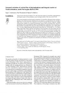
Figure 1. Diurnal VOC fluxes observed during the 3 seasons—spring 2002 (left panel), summer 2002 (middle panel) and fall 2001 (right panel). The gray patched area shows the range of observed fluxes, the blue line is the mean flux for the corresponding season. Isoprene together with measurements of ambient temperature/light levels and biological observations (bud break, leaf stage) were used as a means for distinguishing between the three characteristic seasons: fall, spring and summer. forests. Bigtooth aspen (Populus grandidentata) and trembling aspen (Populus tremuloides) dominate within the footprint of the tower and are the major source for isoprene [Curtis et al., 2002]. The major VOCs detected by PTR-MS were methanol (m/z 33+), acetaldehyde (m/z 45+), acetone (m/z 59+), and isoprene (m/z 69+). The system was run in a flux mode for 30% of the time in fall; for the rest it scanned over a wide range of masses in order to survey any significant presence of unknown VOCs related to senescence. In spring/summer 2001 100% of the measurement time was used for flux measurements. Confirmation of these assignments was also obtained by occasional cartridge sampling and subsequent GC analysis. Tracer compounds for biomass burning (CH3CN) and primary anthropogenic emissions (benzene, toluene) were also assessed, and were in general low with mean mixing ratios in 2001 (2002) around 0.14 (0.21) ppbv, 0.07 (0.06) ppbv and 0.06 (0.07) ppbv, respectively. [6] Methanol: The upper panels in Figure 1 show methanol fluxes in fall (Sept – Nov) 2001 (right), spring (April – May) 2002 (left) and early summer (May – July) 2002 (middle). Isoprene emissions (not shown) together with biological (leaf stage, bud break) and meteorological observations (temperature, light levels) were used as a proxy to distinguish the three characteristic seasons. Only periods with no rainfall were used. The gray patched area depicts the range of observed fluxes with maximum values up to 2.0 mg m 2 h 1 in spring. This mean midday flux of about 1 mg m 2 h 1 in spring and summer are lower than previous observations of fluxes between 2 – 5 mg m 2 h 1

above a ponderosa pine plantation [Schade et al., 2001] and a subalpine coniferous forest [Baker et al., 2000; Karl et al., 2002b]. These conifer forest observations were associated with similar or lower midday temperatures, 12– 18C for the subalpine forest and 17– 23C for the pine plantation, than were observed at the broadleaf forest indicating that the higher emissions were not the result of higher temperatures. The current U.S. EPA biogenic emission model, BEIS 3.11, predicts emissions of 0.27 to 0.56 mg m 2 h 1 for conifer forests with above canopy temperatures between 15 and 23C and emissions of 0.17 to 0.74 mg m 2 h 1 for a broadleaf forest with above canopy temperature ranging from 17 to 33C. These predictions are a factor of 2 – 3 lower than observed for the broadleaf forest. The BEIS 3.11 predictions are based on the Guenther et al. [2000] leaf level emission factors, the Guenther et al. [1995] emission algorithms and the Geron et al. [1994] foliar densities. Mean observed concentrations in fall, spring and summer were 4, 8 and 10 ppbv respectively, with peak maximum concentrations up to 21 ppbv in summer 2002, comparable to values reported by Goldan et al. [1995] above a pine forest plantation in western Alabama and Riemer et al. [1998] during the Southern Oxidant Study. [7] Methanol fluxes followed a logarithmic temperature dependence in the form of Ef x exp(b(T-Ts) (with Ef, basal emissionrate, b, an empirical temperature exponent, Ts, standard temperature 30C) (Table 1). Due to temperature differences between fall 2001 (average T: 13C, maximum T: 24C) and spring/summer 2002 (average T: 17C, maximum T: 33C) fluxes were normalized to a standard temperature (Ts) of 30C allowing for a seasonal intercomparison. Normalized fluxes in spring were 1.7 times higher than in fall. This argues for a significant seasonal dependence with peak emissions during the growing season. A methanol pulse in spring correlates well with a sharp increase of leaf area index (LAI) caused by a late start of bud break in May 2002. [P. Curtis, personal communication]. These results are consistent with the current understanding of methanol production in live plant tissue: formation during cell expansion through demethylation of pectin [Galbally and Kirstine, 2002]. These authors used net ecosystem primary productivity (NPP) to upscale methanol emissions from plants and assumed that 0.10% of NPP is converted to methanol for type I plants (trees). Estimated NPP for the Prophet site was inferred from a detailed biometric study for the years 1999 – 2001 yielding 639 g m 2 y 1 [Curtis et al., 2002]. Assuming that plant growth is minor in fall (setting the part attributed to plant growth to zero for the fall data and taking the combination of the part associated with plant growth and decaying material on the ground for the spring/summer dataset), we apportion 0.084 – 0.10% (C) NPP to demethylation of pectin and 0.116– 0.140% (C) NPP to processes other than cell wall expansion. Our estimate for plant growth falls surprisingly close to the emission factor (0.10%) used by Galbally and Kirstine [2002], however it indicates that the part associated with other processes seems to be significantly underestimated. Warneke et al. [1999] reported emission factors related to plant decay for methanol and gave a best estimate of 0.01 – 0.02% (g(C) gdw 1). They noted, however, that methanol emissions could be much higher up to several milligrams per gram (dw) (e.g., up to 0.188% g(C)


2-3

SDE

Table 1. Summary of Seasonal VOC Emission Patterns Observed at the Prophet Tower in 2001 and 2002 Mixing Ratio 01 mean (max) Mixing Ratio 02 mean (max) Fluxes 01: mean (max) Fluxes 02: mean (max) Ef EPA BEIS 3: max @ 30C Ef 01 b 01 b 02 Ef 02 Ef01 / Ef02 Ci/MeOH ratio: 01 (02) % NPP (% NEE) Source strength [Tg (C) y 1]

Methanol

Acetaldehyde

Acetone

Isoprene

4.2 (15.6)

0.4 (1.6)

1.2 (3.1)

0.1 (1.0)

7.7 (21.0)

0.4 (2.7)

1.9 (5.6)

0.5 (6.0)

0.5 (1.5)

0.3 (1.0)

0.5 (1.6)

0.6 (0.3)

0.9 (2.0)

0.2 (0.7)

0.3 (1.2)

1.0 (7.6)

0.77

0.04

0.07

0.6 (8.4)

0.87 1.50

0.043 0.072 0.58 -

0.20 (0.8) – 0.24 (1.0) 8.9 (6.3 – 11.6)

1.50 0.32

0.123 0.051

4.72 0.02 (0.04) – 0.12 (0.22) 0.1 (0.3) – 0.2 (0.7) 2.7 (2.0 – 3.4)

2.10 0.85

0.099 0.119

2.47 0.22 (0.17) – 0.70 (0.31) 0.1 (0.4) – 0.3 (1.1) 7.0 (3.8 – 10.1)

0.4 (1.6) – 0.8 (3.2) -

a Fluxes (mixing ratios) are reported in mg m 2 h 1 (ppbv). Ef 01, Ef 02 are emission rates (mg m 2 h 1) at a standard temperature of 30 C, b01 (b02) [K 1] is the temperature exponent as described in the text. NEE (net ecosystem exchange), NPP (net primary production). Source strength estimates are based on temperate deciduous and mixed forests defined by the WWF. (www.worldwildlife.org/wildworld)

for 5 mg of methanol per gram dry weight). Assuming that roughly 50% of NPP goes to above ground detritus in temperate ecosystems [Curtis et al., 2002], this would yield emissions up to 0.09% (C) NPP due to decomposition. Considering the influence of other sources (soil, bark) our value for methanol emissions from these sources (0.116 – 0.140% (C) NPP) is somewhat higher, but not completely inconsistent with the previously reported range. The total fraction of methanol emitted from this ecosystem (0.23 ± 0.02% NPP) is much larger than estimated by Galbally and Kirstine [2002] inferring that the upper limit of the biogenic methanol source strength is still poorly constrained as suggested by Heikes et al. [2002]. [8] Acetaldehyde: Acetaldehyde fluxes are shown in Figure 1 center panels. Mean midday fluxes are around 0.27 mg m 2 h 1 in fall (left panel) 0.20 mg m 2 h 1 in spring (middle panel) and 0.3 mg m 2 h 1 in early summer 2002 (right panel) with maximum values up to 1.0 mg m 2 h 1. The U.S. EPA BEIS 3.11 model, described above, underestimates by more than one order of magnitude with predicted acetaldehyde emissions of 0.008 to 0.034 mg m 2 h 1 for a broadleaf forest with above canopy temperature ranging from 17 to 33 C. In addition, our measurements show that the basal emission rate was significantly enhanced in fall (Table 1: Ef01/Ef02 = 4.7) and varied over the seasons. [9] There have been several reports of the release of acetaldehyde from tree leaves under various physiological conditions, including during normal photosynthesis and transpiration [Kesselmeier, 2001], after root flooding [Kreuzwieser et al., 2000], and following light-dark transitions [Holzinger et al., 2000; Karl et al., 2002a]. On a biochemical level, the best understood of these processes is acetaldehyde release that results from the oxidation of ethanol arising in anoxic tissues. Due to the absence of flooding it seems unlikely that the ethanol oxidation mechanism is responsible for the enhanced acetaldehyde emissions in fall 2001. Plant decay may cause higher basal emission rates due to litter fall in autumn. However, Warneke et al. [1999] showed that the acetaldehyde head-

space concentrations from decaying biomaterial were 20– 50 times lower than those of acetone. Since acetaldehyde fluxes observed at the Prophet site were roughly in the same order of magnitude as acetone fluxes, plant decay alone is unlikely to account for the observed enhancement in fall. We draw attention to an alternative production mechanism for acetaldehyde in leaves of woody plants, mentioned above: bursts after light-dark transitions [Karl et al., 2002a] that result from metabolism of accumulated cytosolic pyruvate. In addition, considerable acetaldehyde emissions during crop harvesting (a disruptive process similar to senescence) have been reported recently [deGouw et al., 1999; Karl et al., 2002b]. It seems possible that processes of these types contribute to the increased basal emission rates observed in fall 2001. [ 10 ] Acetone: The concentration range for acetone (Table 1) with maximum values up to 5.6 ppbv in summer 2002 is comparable to that reported by Goldan et al. [1995] and Riemer et al. [1998] at forested sites. Similarly, we observed a rather tight correlation between acetone and methanol with a mean ratio of 0.23 in spring/summer 2002 (range: 0.17 – 0.31) (Goldan: 0.27; Riemer: 0.21), suggesting common sources of acetone and methanol. Assuming the local vegetation is the dominant source of methanol and acetone, this correlation makes sense. Acetone fluxes in spring/summer were roughly a third of methanol (Figure 1), thus the concentration ratio (cacetone/cmethanol) between methanol and acetone would be expected to be close to 0.18 ( = 32/ 58 1/3). The bulk of the fall concentration ratios can be bound between 0.22 and 0.7. The ratio between fluxes of methanol and acetone in fall ranged between 0.5 and 1, which would yield concentration ratios between 0.27 – 0.55. [11] The increased basal emission rate of 2.10 mg m 2 h 1 in fall indicates a substantial enhancement in the late season. Again, BEIS3 substantially underestimates acetone emissions (Table 1). Our data can be compared to emission factors suggested by Warneke et al. [1999] who reported a lower limit of 1.0 x 10 4 g gdw 1, but estimated potential emission factors up to 1.0 10 3 g gdw 1. The acetone yield would therefore be close to 0.03% (C) NPP

SDE

2-4


with 50% of NPP going to aboveground detritus. Assuming a lower limit of 30 days of decaying biomass per year, our best estimate (0.19% (C) NPP) for the forest in Michigan would give a lower limit of 0.036% (C) NPP. Emission factors for decaying plant material reported by Warneke et al., [1999] might therefore be a lower limit for temperate deciduous ecosystems. Our measurements contrast an inverse modeling study on the global acetone budget by Jacob et al., [2002], who scaled the global source strength of decaying biomass down from 9 to 11.2 Tg y 1. The total best estimate (9.5 Tg y 1) for deciduous ecosystems alone inferred from this study is at least a factor of 5 higher than the global total reported by Jacob et al. [2002]. The absence of a large decaying biomass response in their modeling study might be related to the fact that emissions from decomposition follow an exponential temperature dependence. [12] Isoprene: Isoprene emissions at the Prophet tower dominate biogenic VOCs and have been investigated extensively [see Apel et al., 2001 and references within]. Our peak values in early summer 2002 up to 7.6 mg m 2 h 1 (not shown) are comparable to fluxes measured independently [S. Presseley, personnal communication]. Based on our measurements we estimate that total isoprene emissions can account for up to 0.83% (C) NPP (639 g m 2). [13] Total biogenic VOCs from this site: Taking environmental data from 2001 together with our observations we estimate that up to 5.2– 9.9 g (C) m 2 y 1 (0.81 –1.56% (C) NPP) can potentially be lost in form of the four VOCs investigated in this work, with isoprene comprising about half of the total. Using the WWF Terrestrial Ecoregions of the World database (www.world-wildlife.org/wildworld) we estimate the total source strength of methanol, acetone and acetaldehyde for deciduous ecosystems (12 million km2) to be on the order of 8.9 Tg (C) y 1 (12.4 Tg y 1), 2.7 Tg (C) y 1 (5.0 Tg y 1) and 7.0 Tg (C) y 1 (11.2 Tg y 1) respectively. If these estimates are valid, we can conclude that the Earth’s temperate forests are substantial contributors to the atmospheric budget of these oVOCs. [14] Acknowledgments. The National Center for Atmospheric Research is sponsored by the National Science Foundation. This work was also supported in part by NSF grant ATM-0003225, NOAA grant NA06GP0483 and by an Interagency Agreement (DW49939559) from U.S. Environmental Protection Agency. We especially thank M. A. Carroll for use of the Prophet tower facility, P. Curtis, H. P. Schmid and S. Presseley for sharing unpublished results, and the staff of the UMBS research site for their support of this work.

References Apel, E. C., D. D. Riemer, A. Hills, W. Baugh, J. Orlando, I. Faloona, D. Tan, W. Brune, B. Lamb, H. Westberg, M. A. Carroll, T. Thornberry, and C. D. Geron, Measurement and interpretation of isoprene fluxes and isoprene, methacrolein, and methyl vinyl ketone mixing ratios at the Prophet site during the 1998 intensive, J. Geophys. Res., 107, 4034, 2001. Baker, B., A. Guenther, J. Greenberg, and R. Fall, Canopy Level Fluxes of 2-metyl-3-buten-2-ol, acetone and methanol by a portable relaxed eddy accumulation system, Environ. Sci. Technol., 35, 1701 – 1708, 2001. Curtis, P. S., P. J. Hanson, P. Bolstad, C. Barford, J. C. Randolph, H. P. Schmid, and K. B. Wilson, Biometric and eddy-covariance based estimates of annual carbon storage in five eastern North American deciduous forests, Agric. Forest Meteorol., 113, 3 – 9, 2002.

de Gouw, J. A., C. J. Howard, T. G. Custer, and R. Fall, Emissions of volatile organic compounds from cut grass and clover are enhanced during the drying process, Geophys. Res. Lett., 26, 811 – 814, 1999. Galbally, I. E., and W. Kirstine, The production of methanol by flowering plants and the global cycle of methanol, J. Atmos. Chem., 43, 195 – 229, 2002. Geron, C., A. Guenther, and T. Pierce, An improved model for estimating emissions of volatile organic compounds from forests in the eastern United States, J. Geophys. Res., 99, 12,773 – 12,792, 1994. Goldan, P. D., W. C. Kuster, F. C. Fehsenfeld, and S. A. Montzka, Hydrocarbon measurements in the southeastern United States: The Rural Oxidants in the Southern Environment (ROSE) program 1990, J. Geophys. Res., 100, 35,945 – 35,963, 1995. Guenther, A., C. N. Hewitt, D. Erickson, R. Fall, C. Geron, T. Graedel, P. Harley, L. Klinger, M. Lerdau, W. A. McKay, T. Pierce, B. Scholes, R. Steinbrecher, R. Tallamraju, J. Taylor, and P. Zimmerman, A global model of natural volatile organic compound emissions, J. Geophys. Res., 100, 8873 – 8892, 1995. Guenther, A., C. Geron, T. Pierce, B. Lamb, P. Harley, and R. Fall, Natural emissions of non-methane volatile organic compounds, carbon monoxide, and oxides of nitrogen from North America, Atmos. Environ., 34, 2205 – 2230, 2000. Heikes, B. G., et al., Atmospheric methanol budget and ocean implication, Global Biogeochem. Cycles, 16, 1133 – 1146, 2002. Holzinger, R., L. Sandoval-Soto, S. Rottenberger, P. J. Crutzen, and J. Kesselmeier, Emissions of VOCs from Quercus ilex L. measured by PTR-MS under different environmental conditions, J. Geophys. Res., 100, 20,573 – 20,579, 2000. Jacob, D. J., B. D. Field, E. M. Jin, I. Bey, Q. Li, J. A. Logan, R. M. Yantosca, and H. B. Singh, Atmospheric budget of acetone, J. Geophys. Res., 107, 4100, 2002. Karl, T., A. Curtis, T. Rosenstiel, R. Monson, and R. Fall, Transient releases of acetaldehyde from tree leaves-products of a pyruvate overflow mechanism?, Plant Cell Environ, 25, 1121 – 1131, 2002a. Karl, T. G., C. Spirig, J. Rinne, C. Stroud, P. Prevost, J. Greenberg, R. Fall, and A. Guenther, Virtual disjunct eddy covariance measurements of organic compound fluxes from a subalpine forest using proton transfer reaction mass spectrometry, Atmos. Chem. Phys., 2, 279 – 291, 2002b. Kesselmeier, J., Exchange of short-chain oxygenated volatile organic compounds (VOCs) between plants and the atmosphere: A compilation of field and laboratory studies, J. Atmos. Chem., 39, 219 – 233, 2001. Kreuzwieser, J., F. Ku¨hnemann, A. Martis, H. Rennenberg, and W. Urbau, Diurnal pattern of acetaldehyde emission by flooded poplar trees, Physiol. Plant., 108, 79 – 86, 2000. McKeen, S. A., T. Gierczak, J. B. Burkholder, P. O. Wennberg, T. F. Hanisco, E. R. Keim, R. S. Gao, S. C. Liu, A. R. Ravishankara, and D. W. Fahey, The photochemistry of acetone in the upper troposphere: A source of odd-hydrogen radicals, Geophys. Res. Lett., 3177 – 3180, 1997. Riemer, D., et al., Observations of nonmethane hydrocarbons and oxygenated volatile organic compounds at a rural site in the southeastern United States, J. Geophys. Res., 103, 28,111 – 28,128, 1998. Roberts, J. M., F. Flocke, C. A. Stroud, D. Hereid, E. Williams, F. Fehsenfeld, W. Brune, M. Martinez, and H. Harder, Ground-based measurements of peroxycarboxylic nitric anhydrides (PANs) during the 1999 Southern Oxidants Study Nashville Intensive, J. Geophys. Res., 107, 4554, 2002. Schade, G. W., and A. H. Goldstein, Fluxes of oxygenated volatile organic compounds from a ponderosa pine plantation, J. Geophys. Res., 106, 3111 – 3123, 2001. Singh, H. B., Y. Chen, A. Staudt, D. Jacob, D. Blake, B. Heikes, and J. Snow, Evidence from the Pacific troposphere for large global sources of oxygenated organic compounds, Nature, 410, 1078 – 1081, 2001. Warneke, C., T. Karl, H. Judmaier, A. Hansel, A. Jordan, W. Lindinger, and P. J. Crutzen, Acetone, methanol, and other partially oxidized volatile organic emissions from dead plant matter by abiological processes: Significance for atmospheric HOx chemistry, Global Biogeochem. Cycles, 13, 9 – 17, 1999.

R. Fall, CIRES, University of Colorado, Boulder, CO 80309-0216, USA. A. Hansel, Institut fu¨r Ionenphysik, Universita¨t Innsbruck, Austria. T. Karl, and A. Guenther, Atmospheric Chemistry Division, National Center for Atmospheric Research, Boulder, CO, USA. C. Spirig, Eidgenoessische Technische Hochschule, Zurich, Switzerland.