Sensor Validation using Bayesian Networks Ole J. Mengshoel USRA/RIACS NASA Ames Research Center Moffett Field, CA 94035
[email protected]
Adnan Darwiche Computer Science Department University of California Los Angeles, CA 90095
[email protected]
Abstract One of NASA’s key mission requirements is robust state estimation. Sensing, using a wide range of sensors and sensor fusion approaches, plays a central role in robust state estimation, and there is a need to diagnose sensor failure as well as component failure. Sensor validation techniques address this problem: given a vector of sensor readings, decide whether sensors have failed, therefore producing bad data. We take in this paper a probabilistic approach, using Bayesian networks, to diagnosis and sensor validation, and investigate several relevant but slightly different Bayesian network queries. We emphasize that onboard inference can be performed on a compiled model, giving fast and predictable execution times. Our results are illustrated using an electrical power system, and we show that a Bayesian network with over 400 nodes can be compiled into an arithmetic circuit that can correctly answer queries in less than 500 microseconds on average.
1. Introduction The problem of faulty sensors is commonplace in aerospace, leading to a need for sensor validation [2] [1]. Essentially, the sensor validation problem is this: given a vector of sensor readings, decide whether one or more sensors have failed and are therefore producing bad data. Much previous work on sensor validation and failure detection within aerospace has emphasized airand spacecraft control in a continuous setting [21] [18]. Many systems of interest to the aerospace community, for example rocket engines [2] [1] [11] and electrical power systems [3] [12] [19], are either discrete or hybrid (both continuous and discrete) and involve substantial uncertainty. Our focus here is on such systems, and in particular we emphasize those that can be formalized using multivariate discrete random
Serdar Uckun Intelligent Systems Division NASA Ames Research Center Moffett Field, CA 94035
[email protected]
variables represented as Bayesian networks [24]. Our contribution is three-fold. First, we develop a Bayesian network framework for reasoning in which we represent both sensor faults and component faults. Second, we carefully discuss different probabilistic queries that are useful for sensor validation and diagnosis. Third, we investigate the efficient implementation of these ideas, such that they can be implemented and deployed on aerospace vehicles. We take a Bayesian approach to sensor validation [2]. Specifically, our approach is based on developing a Bayesian network (BN) [24] model of an aerospace vehicle or a sub-system of such a vehicle. These models represent the health modes of sensors explicitly, and contain random variables for capturing other aspects of the system (including the health status of other system components). Our approach complements other technologies used in aerospace, including limit checks, redundancy-based voting, and other analytical redundancy methods. Specifically, we advocate an analytical technique that fuses information from multiple sensors in a Bayesian manner, and takes into account relationships between sensors and other system components. To solve the sensor validation problem exactly, we dynamically provide input to the BN using sensor readings and commands and pose a MAP (maximum a posteriori hypothesis) query over the health of sensor variables only [17]. This should be distinguished from alternative approaches formulated within probabilistic frameworks, for instance (i) a MAP computation over the health variables of all system components; (ii) a MPE (most probable explanation) computation over all non-observed system variables; and (iii) a marginal probability computation over each non-observed variable, which can easily be used to find the most likely values (MLVs) of health variables of interest. There are subtle differences between these queries with implications for the decision making process. Our Bayesian framework correctly handles multiple
sensor failures, since it supports reasoning about the joint probability distribution over the health of all sensors; traditional approaches typically depend on marginal probabilities over individual sensor health variables. At the same time, our framework allows us to clearly state and investigate a range of probabilistic queries, both MAP and approximate (but potentially more efficient) probabilistic queries. Finally, we investigate how our approach is supported by efficient algorithms. We report on experiments using an electrical power system [19], and show that a Bayesian network with over 400 nodes can be compiled into an arithmetic circuit that correctly answers queries in less than 500 microseconds on average. The rest of this paper is organized as follows. In Section 2 we discuss related research. Section 3 introduces our Bayesian network framework for sensor validation and diagnosis; we also consider different probabilistic queries. In Section 4 we motivate and illustrate our approach by means of the Mars Polar Lander and electrical power systems. In Section 5 we provide experimental results before concluding in Section 6.
2. Related Work Sensor validation can be considered to be part of the larger effort of improving reliability and safety through the use of redundancy, which can be classified into hardware redundancy, analytical redundancy, and hybrid redundancy [18]. On the hardware side, techniques such as duplex, triplex, or higher hardware redundancy along with voting system are used. Analytical redundancy techniques, further discussed below, can be classified into quantitative methods and qualitative methods. Finally, hybrid methods combine hardware and analytical redundancy. Bayesian networks represent analytical (probabilistic or deterministic) relationships between different states of components and systems, and can therefore be regarded as an analytical redundancy approach. We consider Bayesian and non-Bayesian approaches, and emphasize in this paper the Bayesian approach [24] [2] [16] [6] [20] [7] [17] [15] [13] [14]. We distinguish between work that explicitly represents, using random variables, system health [2] [16] [11] [6] versus work that does not [20] [7]. We now discuss related research, turning first to sensor validation using BNs in aerospace. Bickmore investigates rocket engine sensor data validation [2]. He presents an approach in which a bipartite Bayesian network is constructed from an undirected sensor validation network. Using temperature and pressure
sensors, the approach was successfully tested on space shuttle main engine (SSME) data. More extensive and realistic tests were later performed on a fault tolerant flight computer [1]. Liu and Zhang also developed sensor validation and fault diagnosis techniques for SSME [11]. Theirs is a multi-step approach, involving these steps: Data acquisition, parameter estimation, fault detection, and fault diagnosis. A bipartite BN model – consisting of 9 nodes for sensor readings, 9 sensor health nodes, and 5 component health nodes – is used in the fault diagnosis step only. They report encouraging simulation results, but note that the fault detection module causes a few false and missed alarms. In the area of sensor fusion using BNs, Rehg, Murphy and Fieguth develop, using computer vision algorithms, a speaker detection approach that uses Bayesian networks [20]. They use four “soft sensors”, namely off-the-shelf computer vision algorithms that process skin color, skin texture, frontal face, and mouth motion, and fuse their output by means of a BN. Promising experiments illustrate the benefit of speaker detection using BNs. Hansen et al. discuss sensor fusion using dynamic Bayesian networks (DBNs) [7]. (DBNs are generalizations of Markov chains and hidden Markov models and are used to reason about dynamic processes.) They observe that simple state controllers do not handle faulty sensors, and investigate how DBN sensor fusion can be applied to climate control in buildings. This climate control application uses temperature and humidity sensors; actuation is done by means of ventilation, heating, or cooling. The expectation-maximization (EM) algorithm is used for DBN parameter estimation, and the Boyen-Koller algorithm [23] for computation of marginals. The DBN does not contain health nodes, neither for components nor for sensors. Promising experiments illustrate estimation of temperature from other measurements. Ferrari and Vaghi develop a BNbased sensor fusion approach to mine detection [6]. They consider different types of sensors – specifically ground-penetrating radar, electro-magnetic induction, and infrared sensors – and show how machine learning can be utilized. The sensor model of Ferrari and Vaghi is particularly rich, and their experiments show how sensor fusion using BNs improves landmine classification by 62%. In the area of sensor fusion and diagnosis using BNs, Nicholson and Brady developed a DBN-based approach (DBNs) to solve data association and sensor validation problems [16]. Specifically, they show how DBNs can be used for monitoring robots and humans. For sensor validation, BN nodes representing sensors faults are dynamically added – and then queried – based on the computation of a conflict measure. Lerner et al. develop a hybrid DBN approach to online
monitoring and diagnosis, where nominal as well as failure modes are represented [10]. Burst failures, measurement failures, and parameter drift failures are all represented using discrete BN nodes. During inference, their approach collapses similar hypothesis, thereby avoiding computational complexity issues due to the discrete nodes. In a challenging experiment involving multiple faults in a system of five liquid tanks, they report strong results. Compared to previous research, including work that explicitly represents nominal and faulty behavior using Bayesian network nodes [16] [10] [6], we carefully introduce a Bayesian network framework and emphasize the different results produced by marginal, MPE, and MAP queries. In contrast, all previous sensor validation work we are aware of has employed marginals. We also do not rely on computation of residuals [18] or a separate fault detection step [21] [11]. Instead, we go directly to a diagnosis or sensor validation step (similar to [10] [7]); fault detection has been identified as a cause of false and missed positives [11]. We emphasize that on-line inference including sensor validation can be performed on a compiled model, not directly on the Bayesian network. Compilation of BNs gives fast and predictable execution times [9] [4], which enable deployment in the real-time and resource-bounded environments typically found in aerospace vehicles [5] [13]. Finally, we note that our Bayesian approach can utilized in distributed architectures with smart sensors [22], even though space does not permit us to discuss detailed here.
3. Bayesian Network Framework We now discuss our Bayesian network model for an aerospace vehicle. (Note that our approach generalizes to systems beyond vehicles of interest to NASA, but in the interest of specificity we use the term “vehicle” rather than “system” here.) This model constitutes a Bayesian approach to sensor fusion and validation, and it represents the health state of a vehicle’s sensors and other components. Specifically, we partition the set of BN nodes X into HV, E, and R as follows: • Health nodes (HV), where HV = HC ∪ HS and HC ∩ HS = ∅, with: – Component health nodes (HC): Nodes representing health of vehicle components (excluding health of sensors). – Sensor health nodes (HS): Nodes representing health of vehicle’s sensors. • Evidence nodes (E), where E = EC ∪ ES and EC ∩ ES = ∅, with:
–
•
Command nodes (EC): Nodes representing commands to vehicle. – Sensor nodes (ES): Nodes representing sensor readings from vehicle. Remaining nodes (R): Nodes that are not health or evidence nodes. If X is the set of all BN nodes, then R = X - HV – EV.
Such a BN model can be used for Bayesian sensor fusion and sensor validation, as illustrated in Section 4 and Section 5. Different probabilistic queries are used in BNs. Given evidence, computation of marginals is concerned with the posterior belief over individual BN nodes, while finding an MPE produces the most probable explanation over all non-evidence nodes [24]. Less known than the marginal and MPE queries are perhaps maximum a posteriori hypothesis (MAP) queries [17]. Let X be all BN nodes, E the evidence nodes, and e the evidence. Then we might be interested in the MAP over M ⊆ X - E, and use the notation M = m to mean that m is an instantiation of all the nodes in M. For MAP instantiation we say MAP(M, e) = argmaxmPr(M=m, e) = argmaxmPr(M=m | e). Algorithms for efficiently computing MAP have recently been developed [17]. Previous sensor validation efforts have generally computed marginals. Given the concepts introduced above, we can in fact identify several related but different probabilistic queries of interest to diagnosis and sensor validation (the ordering is arbitrary): 1. Health of vehicle query. MAP over the health variables of all vehicle components and sensors: MAP(HV, e). 2. Health of components query. MAP over the health variables of vehicle components only: MAP(HC, e). 3. Health of sensors (or sensor validation) query. MAP over sensor health variables: MAP(HS, e). 4. State of vehicle query. MPE over all non-observed system variables: MAP(X – EV, e) = MPE(e). MPE can be used to obtain an approximation MAPMPE of MAP as discussed below. 5. Health of vehicle marginals. Marginal (belief) over any health variable H: B(H, e) = Pr(H | e) , where H ∈ HV. From B(H, e), it is easy to compute the most likely value of H given e, or MLV(H , e). Using MLV, we can approximate MAP, using MAPMLV, as discussed below. There are subtle differences between these queries with possible implications for the decision making process. In fact, examples of MAP, MPE, and MLV
giving different results over query variables X are known; Section 4 provides an EPS example. Intuitively, the differences between MAP, MPE, and marginal queries are as follows. (Note that MAP is a generalization of MPE and MLV, and hence when we say “MAP queries” in the following we mean MAP queries that are not MPE or MLV queries.) We first discuss marginals versus MPE and MAP. Marginal queries are local, since they are concerned with individual BN nodes. MPE and MAP, on the other hand, are more global and take constraints that involve multiple BN nodes into account. This difference is potentially important in diagnosis and sensor validation because there can be node states that marginally look most likely, but when considered jointly (by MAP or MPE) they are in fact not the most likely. For instance, a state x of one node X ∈ X – E may be highly uncorrelated with a state y of a different node Y ∈ X – E, even though these two states are marginally most likely for X and Y respectively (see Section 4.2 for a concrete example). Second, and considering MAP versus MPE queries, we note that MPE queries are concerned with all non-evidence nodes X – E, while with MAP we query a subset M ⊆ X – E of the nonevidence nodes. Consequently, MPE typically includes states of nodes that are not essential to the component health HC or sensor health HS, which are our main concern in this article. Along an orthogonal dimension, we note that one probabilistic query can be used to approximate another probabilistic query. Specifically, MPE and MLV queries can be used to approximate MAP queries. We use the notation MAPMPE(H, e) and MAPMLV(H, e) to indicate MPE- and MLV-approximations of MAP(H, e). Here, H = HV, H = HC, or H = HS. Such approximations are of both theoretical and practical interest. Theoretically, the MAP problem belongs to a more difficult complexity class than the MPE and marginal problems [17], and even the latter problems can be computationally very challenging [15] [14]. Practically, algorithms and software for MPE and marginal computation are more wide-spread than those for MAP computation. When do these approximations give different results than MAP? This question is explored in the following sections.
4. NASA Applications State estimation methods may be studied from different perspectives, including the mission phase and the subsystem perspectives. Examples of subsystems of great interest to NASA include rocket engines [2] [1] [11] and electrical power systems [3] [12] [19]; mission phases include vehicle takeoff and landing.
In Section 4.1 we turn to a vehicle landing example of why NASA needs better state estimation methods. In Section 4.2 we then discuss electrical power systems and show how BNs can be used in this setting.
4.1 Mars Polar Lander We present the Mars Polar Lander, discuss its failed mission, and speculate how the outcome could have been different if better sensor fusion and sensor validation techniques had been in place. The main purpose of the Mars Polar Lander (MPL) was to collect samples of Mars’ soil. MPL was launched on January 3, 1999; it lost contact with Earth on December 3, 1999. The cause of MPL loss is not known with certainty. According to the Accident Report, however, the most probable cause is premature shutdown of descent engines [8]. It is important to note that MPL was designed for a soft landing (similar to Apollo lunar landers). To enable a soft landing, MPL used a descent engine (retrorocket) to decelerate during descent. Here is a probable sequence of events that led to the loss of the spacecraft [8]: 1. During the descent, a radar altimeter continuously measured height above surface. 2. When a certain height above surface (50 ft.) was reached, the legs of the spacecraft were commanded to deploy. 3. The legs deployed and locked into position, causing a transient on contact sensor(s) that were installed on the legs. 4. The contact sensor transient caused the descent engine controller to (erroneously) infer that the spacecraft had touched down on Mars. 5. The descent engine was shut off prematurely, causing the spacecraft to crash from a height of ~50 ft and be destroyed. In retrospect, it is clear that MPL had enough instrumentation onboard to enable robust state estimation. Height above surface was the critical state variable, and the radar altimeter combined with the touchdown (contact) sensors would have enabled a better estimate of height above surface had the two readings been fused by using a BN model. We want to make the following two points regarding the MPL accident. First, there are multiple direct or indirect measurements of a state variable of interest. Consequently, there is an opportunity to fuse these multiple observations or sensor readings using an analytical model, in our case a BN. Second, there is a need to query the BN in order to find conflicts and causes of conflicts in sensor readings, and then to decide which sensor reading(s) to trust. For the MPL,
CommandRelay (CR)
HealthRelay (HR) Prob.
Prob. open
0.5
close
0.5
CR
HR
SR
healthy
0.999
stuckOpen
0.0005
stuckClosed
0.0005
HealthSensor (HS)
HS
Prob.
FS StatusRelay (SR) HR CR
healthy open
healthy
0.999
stuckOpen
0.0005
stuckClosed
0.0005
stuckOpen close
open
stuckClosed
close
open
close
open
1.0
0.0
1.0
1.0
0.0
0.0
closed
0.0
1.0
0.0
0.0
1.0
1.0
FeedbackSensor (FS) HS SR
healthy open
stuckOpen closed
open
stuckClosed
closed
open
closed
readOpen
1.0
0.0
1.0
1.0
0.0
0.0
readClose d
0.0
1.0
0.0
0.0
1.0
1.0
Figure 1. Bayesian network representing an electrical power system relay.
one sensor (the contact sensor) indicated touchdown, while another sensor (radar altimeter) did not indicate touchdown. A BN model could have been used to resolve this conflict by explicitly reasoning about the health of these sensors, using the probabilistic queries discussed in Section 3.
4.2 Electrical Power Systems Electrical power systems (EPSs) play an essential and increasing role in aerospace vehicles [3] [12] [19]. EPS loads include avionics, propulsion, life support, and thermal management. For the purpose of this paper, the EPS components we are interested in include batteries, relays, circuit breakers, and EPS loads such as light and pumps. For EPSs, sensors include voltage sensors, current sensors, and load sensor such as temperature and light sensors. Here is a simple example of EPS operation. Suppose that a vehicle crew member issues a command to a relay in a vehicle’s EPS. If the relay is healthy, the command changes the status of the relay – from open to closed, or from closed to open. There is also a feedback element that – if healthy – reports back the actual relay state to the crew member. Now suppose that the crew member gives a “close relay” command, resulting in a “relay open” feedback message. There is
an inconsistency here, since the relay was commanded to close, but the feedback says that it is open! Figure 1 shows how this simple example can be formalized using a BN. The BN expresses how the status of the relay, StatusRelay (SR), depends on the health of the relay, HealthRelay (HR), as well as the command given to it, CommandRelay (CR). Further, the message from the relay’s feedback sensor, FeedbackSensor (FS), is determined by the status of the relay as well as its health, HealthSensor (HS). Using the framework established in Section 3, we have HC = {HealthRelay}, HS = {HealthSensor}, EC = {CommandRelay}, ES = {FeedbackSensor}, and R = {StatusRelay}. To reflect the command from the crew member, we clamp CommandRelay to close in the BN, while the feedback we get from the EPS is that the relay is open, thus we clamp FeedbackSensor to readOpen. Using this BN and the above evidence, we can explore possible reasons for the inconsistency. We employ the five probabilistic queries from Section 3 and obtain the following results: 1. Health of vehicle query. MAP(HV, e) = {HealthRelay = stuckOpen, HealthSensor = healthy} and MAP(HV, e) = {HealthRelay = healthy, HealthSensor = stuckOpen}. These two answers have the same probability. 2. Health of components query. MAP(HC, e) = {HealthRelay = stuckOpen}. 3. Health of sensors (or sensor validation) query. MAP(HS, e) = {HealthSensor = stuckOpen}. 4. State of vehicle query. MAPMPE(HV, e) = {HealthRelay = healthy, HealthSensor = stuckOpen}. This approximation is the same as one of the MAP(HV, e) results above. 5. Health of vehicle marginals. MAPMLV(HV, e) = {HealthRelay = stuckOpen, HealthSensor = stuckOpen}. This approximation is different from both of the MAP(HV, e) results above. Suppose that we are interested in HV = HC ∪ HS = {HealthRelay, HealthSensor}, and consider MAP(HV, e). Intuitively, this query considers combinations of values for both HealthRelay and HealthSensor. However, when each health node in HV is considered in isolation, as it is in MAPMLV(HV, e) above, incorrect approximations can result. We note that both the two last queries above are approximations of MAP(HV, e). When we take MAPMLV(HV, e) in Query 5 above, we obtain two unhealthy nodes. This is different from all the other queries above. This is an interesting example of how naively computing the MLVs over HV to approximate MAP(HV, e) does not always give the desired answer.
Table 1. Experimental results for ADAPT testbed. ID
Injected Fault and Location
MAP(HV, e),MAP e MPE (H V,,e), and MAP MLV (H V ,,e)
MAP(HC , e)
MAP(HS , e)
Relay Failed Open, 304 EY260
Health_relay_ey260_cl = stuckOpen
Health_relay_ey260_cl = stuckOpen
Relay Feedback 305 Sensor Failed, ESH175
Health_relay_ey175_cl = stuckOpen
Health_relay_ey175_cl = stuckOpen
Circuit Breaker 306 Tripped, cbISH262
Health_breaker_ey262_ op = stuckOpen
Health_breaker_ey262_ op = stuckOpen
Voltage Sensor Failed, 308 E261
Health_e261 = stuckVoltageLo
Health_e261 = stuckVoltageLo
Load Sensor Failed, 311 LT500
Health_LT500 = stuckLow
Health_LT500 = stuckLow
5. Experiments What are the differences, if any, between using the probabilistic queries MAPMPE(HV, e), MAPMLV(HV, e), MAP(HV, e), MAP(HC, e), and MAP(HS, e) in more realistic applications? What are the execution times? To explore these questions, we now report on experiments using data from the Advanced Diagnostics and Prognostics Testbed (ADAPT) [19]. ADAPT is a facility developed at NASA Ames for supporting the development of diagnostic and prognostic models; for evaluating advanced warning systems; and for testing diagnostic and prognostic tools and algorithms. ADAPT is an electrical power system (EPS) with components for power generation, storage, and distribution. Over a hundred sensors report their measurements to health management systems that monitor the status of the EPS. For the purposes of diagnosis and sensor validation, we have developed an ADAPT BN which contains a total of 432 nodes. The ADAPT BN reflects the testbed and is developed according to the framework presented in Section 3. There are 122 nodes in HV, 57 nodes in HC, and 65 nodes in HS. The BN combines BN fragments representing individual EPS components, similar to the relay discussed in Section 4.2, into a representation of power storage, distribution, and loads in ADAPT. ADAPT provides an environment in which to inject failures in a controlled manner, and this makes it ideal for use in sensor validation and diagnosis experiments.
For each experiment considered here (see Table 1), the location and type of the injected fault is presented. Component failures are injected in experiments 304, 305, and 306, while sensor failures are injected in experiments 308 and 311. Experiments were performed using the SamIam and ACE software tools (see http://reasoning.cs.ucla.edu/). Results from the experiments are presented in Table 1. Only BN nodes with non-healthy states are presented in this table. We have also merged the results for the queries MAP(HV, e), MAPMPE(HV, e), and MAPMLV(HV, e), since they turned out to be the same (in general they will not be, as we saw in Section 4.2). Perhaps the most interesting observation in Table 1 is how the results are the same across the different probabilistic queries. In some ways this is good news, since it suggests that the faster and more common MAPMPE(HV, e) and MAPMLV(HV, e) probabilistic queries can sometimes be good approximations to MAP for BNs like the ADAPT BN. Since aerospace vehicles often have stringent realtime and resource requirements, we are interested in the arithmetic circuit execution times of ACE. In Figure 2, statistics for ACE inference times for the MAPMPE(HV, e) and MAPMLV(HV, e) queries are summarized. These measurements were made on a PC with an Intel Pentium 4 3.2 Ghz processor, 1 GB RAM, and Windows XP Pro. The inference time statistics are based on all probabilistic queries during an experimental run. For both query types, the benefit of compilation to an arithmetic circuit is clearly
ADAPT Experiments - MPE Run Times
Run time (millisec)
100.000 10.48
10.39
10.41
10.34
10.45
10.000
Mean Median
1.000
0.384
0.471
0.360
0.443
0.478
Maximum
0.100 304
305
306
308
311
ADAPT Experiment ID
ADAPT Experiments - MLV Run Times
Run time (millisec)
100.000 12.18
12.04
12.06
12.08
11.99
10.000
Mean Median
1.000
0.368
0.472
0.315
0.435
0.455
Maximum
0.100 304
305
306
308
311
system setting, our experiments showed that MAP approximation based on marginals and MPE can in fact give very good results. Our Bayesian formulation has several theoretical and practical benefits. Theoretical benefits include: the solid foundation of Bayesian networks in probability and graph theory; a compilation approach that creates fast and predictable vehicle health management systems in embedded and resourcebounded settings (for details see [5] [4] [13]); and the fact that Bayesian networks generalize techniques – such as Kalman filters, fault trees, and hidden Markov models – that are already well-established in the aerospace community. Practical benefits include: The existence of a plethora of academic and commercial software tools that implement Bayesian networks and their inference algorithms; general but efficient BN inference algorithms that provide a foundation for sensor fusion and sensor validation; and the ability of BNs to enable cross-fertilization and integration between different application areas and subsystems.
ADAPT Experiment ID
Figure 2. Execution times for ADAPT Bayesian network after it has been compiled into an arithmetic circuit.
demonstrated: The query evaluations are very fast, specifically in the 300-500 microseconds range (on average) for the compiled ADAPT BN. In addition, query execution is predictable, which is crucially important for real-time applications. Predictability is expected to further increase once a real-time operating system is used.
6. Conclusion In this paper, we have provided a framework for sensor validation and diagnosis using a Bayesian network approach. The framework has been applied to an electrical power system, an essential subsystem in aerospace vehicles [3] [19]. We advocate an analytical technique that (i) fuses information from multiple sensors and (ii) takes into account relationships between sensors and other system components. We identify five different probabilistic queries, including a MAP query that correctly handles multiple sensor failures as it explicitly reasons about the joint probability distribution over all sensor health variables, compared to traditional approaches that typically depend on marginal probabilities over individual sensors. We also discuss approximations using marginals and MPE. While we give an example of marginals performing poorly in our electrical power
7. Acknowledgments This material is based upon work supported by NASA under contract NNA07BB97C ISRDS. The help of Keith Cascio, Mark Chavira, and Scott Poll related to ADAPT and running the ADAPT BN experiments is also greatly appreciated and acknowledged.
8. References [1] R. L. Bickford, T. W. Bickmore, and V. A. Caluori, “Real-Time Sensor Validation for Autonomous Flight Control”, In Proc. 33rd Joint Propulsion Conference and Exhibit, Seattle, WA, July 1997. [2] T. W. Bickmore, “A Probabilistic Approach to Sensor Data Validation”, In Proc. 28th Joint Propulsion Conference and Exhibit, Nashville, TN, July 1992. [3] R. M. Button and A. Chicatelli, “Electrical Power System Health Management”, In Proc. 1st International Forum on Integrated System Health Engineering and Management in Aerospace, November 2005, Napa, CA. [4] M. Chavira and A. Darwiche, “Compiling Bayesian Networks Using Variable Elimination”, In Proc. of the 20th International Joint Conference on Artificial Intelligence (IJCAI-07), January 2007, pp. 2443 – 2449. [5] A. Darwiche, “Model-Based Diagnosis under Real-World Constraints”, AI Magazine, Vol. 21, No. 2, 2000, pp. 57-73.
[6] S. Ferrari and A. Vaghi, “Demining Sensor Modeling and Feature-Level Fusion by Bayesian Networks”, IEEE Sensors Journal, Vol. 6, No. 2, April 2006. [7] J. A. Hansen, T. D. Nielsen, and H. Schiøler, “Sensor Fusion using Dynamic Bayesian Networks in Livestock Production Buildings”, In Proc. of the International Conference on Computational Intelligence for Modelling, Control and Automation (CIMCA06), 2006. [8] JPL Special Review Board, “Report on the Loss of the Mars Polar Lander and Deep Space 2 Missions”, JPL Special Review Board Report, March 2000. [9] S. Lauritzen and D. J. Spiegelhalter, “Local Computations with Probabilities on Graphical Structures and their Application to Expert Systems (with Discussion)”, Journal of the Royal Statistical Society series B, Vol. 50, No. 2, 1988, pp. 157-224. [10] U. Lerner, R. Parr, D. Koller, and G. Biswas, “Bayesian fault detection and diagnosis in dynamic systems”, In Proc. of the Seventeenth National Conference on Artificial Intelligence (AAAI-00), 2000, pp. 531–537. [11] E. Liu and D. Zhang, “Diagnosis of Component Failures in Space Shuttle Main Engines using Bayesian Belief Networks: A Feasibility Study”, In Proc. 14th IEEEE International Conference on Tools with Artificial Intelligence (ICTAI-02), 2002. [12] W. A. Maul, K. J. Melcher, A. K. Chicatelli, and T. S. Sowers, “Sensor Data Qualification for Autonomous Operation of Space Systems”, In AAAI Fall Symposium on Spacecraft Autonomy: Using AI to Expand Human Space Exploration, Arlington, VA, October 2006. [13] O. J. Mengshoel, “Designing Resource-Bounded Reasoners using Bayesian Networks: System Health Monitoring and Diagnosis”, In Proc. of the 18th International Workshop on Principles of Diagnosis (DX-07), Nashville, TN, May 2007. [14] O. J. Mengshoel, “Macroscopic Models of Clique Tree Growth for Bayesian Networks”. In Proc. of the 22nd National Conference on Artificial Intelligence (AAAI-07). July 2007, Vancouver, Canada, pp. 1256-1262.
[15] O. J. Mengshoel, D. C. Wilkins, and D. Roth, “Controlled Generation of Hard and Easy Bayesian Networks: Impact on Maximal Clique Tree in Tree Clustering”. Artificial Intelligence, 170(16–17), October 2006, pp. 1137–1174. [16] A. E. Nicholson and J. M. Brady, “Dynamic Belief Networks for Discrete Monitoring”, IEEE Trans. on Systems, Man, and Cybernetics, Vol. 24, No. 11, November 1994. [17] J. D. Park and A. Darwiche, “Complexity Results and Approximation Strategies for MAP Explanations”, Journal of Artificial Intelligence Research (JAIR), Vol. 21, 2004, pp. 101-133. [18] R. J. Patton, “Fault detection and diagnosis in aerospace systems using analytical redundancy”, Computing & Control Engineering Journal, Vol.2, No.3, May 1991, pp.127-136. [19] S. Poll, A. Patterson-Hine, J. Camisa, D. Garcia, D. Hall, C. Lee, O. J. Mengshoel, C. Neukom, D. Nishikawa, J. Ossenfort, A. Sweet, S. Yentus, I. Roychoudhury, M. Daigle, G. Biswas, and X. Koutsoukos, “Advanced Diagnostics and Prognostics Testbed”, In Proc. of the 18th International Workshop on Principles of Diagnosis (DX-07), Nashville, TN, May 2007. [20] J. M. Rehg, K. P. Murphy, P. W. Fieguth, “VisionBased Speaker Detection Using Bayesian Networks”, In Proc. 1999 Conference on Computer Vision and Pattern Recognition (CVPR-99), June 1999, Ft. Collins, CO, pp. 2110-2116. [21] A. S. Willsky, “A Survey of Design Methods for Failure Detection in Dynamic Systems”, Automatica, Vol. 12, 1976, pp. 601-611. [22] F. Figueroa and J. Schmalzel, “Rocket Testing and Integrated System Health Management”, In Condition Monitoring and Control for Intelligent Manufacturing, W. Gao (ed), Springer Verlag, 2006, pp. 373-392. [23] D. Koller and X. Boyen, “Exploiting the Architecture of Dynamic Systems,” In Proc. of the 16th National Conference on Artificial Intelligence (AAAI-99), July 1999, pp. 313-320. [24] J. Pearl, “Probabilistic Reasoning in Intelligent Systems: Networks of Plausible Inference”, Morgan Kaufmann, 1988.