Recurrence and Cross Recurrence Plots Reveal the Onset of the Mulde Event (Silurian) in the Abundance Data for Baltic Conodonts Andrej Spiridonov* Department of Geology and Mineralogy, Vilnius University, M. K. Čiurlionio 21/27, LT-03101 Vilnius, Lithuania
ABSTRACT One of the severest perturbations of the Silurian marine environment is the mid-Homerian Mulde bioevent. This event proceeded in several temporal steps, which, according to some authors, implies possible globally synchronous perturbation. The dynamic pace and consequences of these perturbations, as well as their effects on conodont community dynamics, are largely unknown. Here I used so-called recurrence and cross recurrence plots to test the hypothesis of common forcing of the Mulde event on conodont abundance dynamics at the regional scale. The results of the analysis of two Lithuanian sections from the Baltic basin revealed that in the uppermost part of the lundgreni graptolite biozone there was sharp transition in the recurrence patterns. Pre-Mulde Homerian time was characterized by high-amplitude fluctuations and a low recurrence rate. On the other hand, the Mulde interval state was characterized by low abundance and a high recurrence rate with longer horizontal, vertical, and diagonal lines of the recurrence plot, which implies transition to a more ordered (irregularly periodic), stable (laminar) dynamical state. The cross recurrence plot analyses of Lithuanian and Polish core data show a close coherence of this pattern at the regional scale, which is expected for widespread critical transition in ecosystem structure. Additionally, with appropriate regression techniques, cross recurrence plots of conodont abundance allow correlation of sections without prior input from other kinds of stratigraphical information. This shows the potential of conodont abundance as a potent tool in revealing the effects of the Mulde event at the regional scale and coherent dynamical patterns of recurrence that can inform stratigraphic correlation. Online enhancement: supplemental table.
Introduction The fossil record reveals that bioevents of varying magnitude are a salient feature of the history of life (Raup and Sepkoski 1982; Foote 2005; Bambach 2006). The Silurian period was an environmentally and macroevolutionary volatile time interval (Cooper et al. 2014; Crampton et al. 2016), punctuated by many oceanic biogeochemical events (Jeppsson 1987, 1998; Saltzman 2005; Lenton et al. 2016). Of particular importance is the Mulde bioevent (Upper Wenlock), which resulted in a substantial loss of graptolite species (Melchin et al. 1998; Cooper et al. 2014; Radzevičius et al. 2014b), a significant turnover of conodont taxa (Aldridge et al. 1993; Jeppsson and Calner 2002; Radzevičius et al. 2016), and large carbon cycle perturbations expressed by a double-peaked
carbon isotopic excursion (Samtleben et al. 1996; Martma et al. 2005; Cramer et al. 2006; Jarochowska et al. 2015). High-resolution analyses of conodont extinctions and extirpations during the Mulde event indicated the possibility that “datums,” or event levels of conodont turnover, could be recognized globally (Jeppsson 1998). According to Jeppsson, these datums represent (presumably) externally forced oscillations during transitions between alternative oceanic states. It was suggested that the Mulde and other transitions in this model are direct reflections of the Milankovitch forcing of the Earth’s system, which induces rapid alternation between two circulation regimes, one driven by warm but saline dense water, the other by cold dense water (Jeppsson 1997; Calner 2008). These transitions or alternations are hypothesized to destabilize ecosystems by disturbing productivity and habitats (Aldridge et al. 1993). Additional disturbances could be related to periodic and
Manuscript received September 10, 2016; accepted January 10, 2017; electronically published March 23, 2017. * E-mail:
[email protected].
[The Journal of Geology, 2017, volume 125, p. 381–398] q 2017 by The University of Chicago. All rights reserved. 0022-1376/2017/12503-0007$15.00. DOI: 10.1086/691184
381
382
A. SPIRIDONOV
episodic changes in water mass chemistry (or even toxicity; Vandenbroucke et al. 2015), to which conodonts were apparently sensitive (Herrmann et al. 2015), and to changes in overall ecosystem productivity driven by changes in upwelling (Spiridonov et al. 2016). Whatever the ultimate reasons for these inferred (quasi-)periodic extinction steps, they are evidently taxonomically recognizable in geographically widely distributed stratigraphic records (Cramer et al. 2011; Molloy and Simpson 2012). The best evidence that the Silurian events are composed of datum points comes from the Baltic basin (Jeppsson and Männik 1993; Calner and Jeppsson 2003). If the extinctions proceeded in several synchronous episodes as proposed (Jeppsson 1998), with the abundance of widely distributed species falling to zero, there must have been geographically widespread, synchronous fluctuations in population sizes. Adverse conditions drive certain species to extinction, force others to adapt, and claim a high demographic toll on closely related surviving species (Kirkpatrick 2010). In this way, a whole clade, which shares fundamental physiological and anatomical similarities, should react in concert to strong perturbations. Thus, if this hypothesis is true, we should expect to observe a coherent pattern in fluctuations of conodont abundance during the Mulde event at different localities in the same region and possibly beyond. In order to test this hypothesis, I employed a set of nonlinear time series techniques, developed in the dynamical systems community, and previously unexplored by paleobiologists—so-called recurrence plot and cross recurrence plot analyses— together with supplementary null model testing, for conodont abundance data from two Lithuanian locations and one from the Polish location in the Silurian Baltic basin. Additionally, I explored the potential of the cross recurrence plots for correlation using only abundance data. Recurrence and cross recurrence plots have proved their potential for disentangling dynamical transitions in key variables in a wide range of complex systems research, from detection of brain state changes (Stam 2005) to critical responses in geomorphic systems (Trauth et al. 2003; Vařilová et al. 2011) and shifts in seismic regime (Chelidze and Matcharashvili 2015). This study presents the evidence that paleontological abundance data can locate changes in dynamic regime even before the large-scale changes can be detected in taxonomic composition and stable carbon isotope time series, even with limited sample sizes. Geological Setting and Conodont Data. For the purposes of analysis, I studied the trends in conodont abundance in parts of two Lithuanian cores: Vilkaviški-134 (692.6–780-m depth interval; 60 collections; Radzevičius et al. 2016; see table S1, avail-
able online) and Ledai-179 (629.9–705.6-m depth interval; 41 collections; Spiridonov et al., forthcoming). The selected intervals extended from the middle part of the Homerian to the middle portion of the Mulde event, namely, the upper Jaagarahu and the lower and middle Gėluva regional stages (Radzevičius et al. 2014, 2016). These wells occur in the shallow facies zone of the eastern part of the Silurian Baltic basin (fig. 1). They were previously the subject of detailed integrated stratigraphic study (Radzevičius et al. 2014, 2016) and age determinations. In addition, in order to test the robustness of the revealed patterns, I compared the conodont abundance trends in the published eastern Polish Widowo IG-1 section material (46 collections from a 562.5–520.25-m interval; Jarochowska and Munnecke 2015). That section apparently spans a more restricted stratigraphic interval (the upper Wenlock Mulde bioevent). By a graphic correlation with the Viduklė-61 section as a reference (Radzevičius et al. 2014b), I projected graptolite zones into the Vilkaviškis-134 and Ledai-179 sections. The minima and maxima of the two positive Mulde carbon isotopic excursions served as correlation points (similar to Sadler 2012). In order to accommodate the nonlinear accumulation, I used second-order polynomial regression in the graphic correlation. Smoothened versions of d13C were used in finding onsets (starts of the rises), maximal values, and endings of the two major Mulde peaks. The identity of peaks in the Viduklė-61 core was confirmed by graptolite and conodont occurrences. For the lower part of the carbon isotopic excursion in the Vilkaviškis-134 core, the identity of the peaks was confirmed by graptolites. Conodonts confirmed the upper part. In the Ledai-179 core, the identity of both Mulde peaks was confirmed by the conodont taxa data. In all three sections, carbon isotopic and conodont records extend through mid- and upper Homerian strata and into the Ludlow, which assures the accuracy of the recognition of excursion boundaries. The base of the Mulde event is here accepted as the top of the lundgreni biozone, which marks a major extinction of graptolites (Melchin et al. 1998). The sampled interval from the two cores spans from the upper part of the lundgreni to the middle part of the deubeli graptolite zones. The uppermost part of the Homerian was not studied here, because in the Vilkaviškis-134 and Ledai-179 cores it is represented by very restricted environments (sabkhas and lagoons), which show very different paleoecological and taphonomic environments with very rare conodonts in comparison to the main part of the record (Radzevičius et al. 2014, 2016). As a proxy for the original abundance of conodonts at the sampling sites, I used the normalized total
Journal of Geology
CONODONT ABUNDANCE DURING THE MULDE EVENT
383
Figure 1. A, Paleogeographic settings (Einasto et al. 1986); graptolite zones and regional stages, with the shaded portion showing the studied interval (Radzevičius 2006). Changes in the abundances of mid-Homerian conodont elements per kilogram of rock in the Villkaviškis-134 (B), Ledai-179 (C; Spiridonov et al., forthcoming), and Widowo IG-1 (D; Jarochowska and Munnecke 2015) cores.
number of conodont elements in the samples. The abundance of conodont elements should be approximately proportional to the number of organisms, because the element numbers in the apparatuses vary within a very narrow range (15–19 elements per apparatus; Purnell and Donoghue 2005; Dzik 2016), and conodonts retained one set of elements throughout their lives (Donoghue and Purnell 1999). Moreover, in all three sections, through the whole studied interval, the numerically dominant genera were Panderodus and Wurmiella, with smaller numbers of
Ozarkodina (closely related to Wurmiella) and several other numerically subordinate genera. It has been shown that this measure is capable of revealing the mechanisms of regional and worldwide geobiological perturbations (Girard and Renaud 2007; Spiridonov et al. 2015, 2016). This approach is similar to the use of fish ichthyolites as a proxy for the paleoproductivity of a clade (Sibert et al. 2016). In order to mitigate bias due to sample size, I calculated the abundance of conodonts per kilogram of rock in the Vilkaviškis-134 core samples, and a
384
A. SPIRIDONOV
similar procedure was carried out on the data of Jarochowska and Munnecke (2015). Unfortunately, the weights of the Ledai-179 samples were not recorded. It was still necessary to bring both sets of collections to the same scale. Therefore, I normalized the abundances from the Ledai-179 well using the average sample mass of the Vilkaviškis134 samples (311 g). Both cores had been sampled using the same sampling procedure (A. Brazauskas, pers. comm.). In any case, the preservation of the signal, in this case the correlation between the standardized and nonstandardized conodont abundances of the Vilkaviškis-134 section (r 2 p 0.94) and also the Widowo IG 1 section (r 2 p 0.83), are very high. Evidently, the signal is well preserved even in nonstandardized data, collected and identified by different researchers. Finally, in order to obtain equally spaced stratigraphic sample series before the analysis, I interpolated the abundance time series at even intervals of 0.5 m. Recurrence Plot Techniques. Recurrence plots are square matrices in which each successive position in a time series is compared to every other position in the same time series and the diagonal of the matrix compares each part to itself. Cells in this matrix are shown in black where differences between the corresponding time series values are smaller than a filtering threshold. In its simplest form, a recurrence plot is a filtered matrix of differences between time series values that are transformed into the binary states, black where similar versus white where different. Rectangular cross recurrence plots compare two different time series in a manner analogous to Alan Shaw’s (i.e., Shaw 1964) graphic correlation of stratigraphic sections. Recurrence plot analysis was introduced to theoretical physics as a way of reconstructing a system’s dynamical properties from the observed time series (Eckmann et al. 1987; Marwan et al. 2007). This approach later found successful applications in other fields of science that study the temporal and spatial behavior of complex and frequently nonlinear systems (Marwan and Webber 2015). The main diagonal line shows recurrence of a state to itself and is therefore always black. Points that lie above the diagonal show recurrence patterns from the given point forward in time; points below the main diagonal represent recurrence patterns backward in time. Recurrence plots allow efficient visual analysis of dynamical patterns because they display relatively easily recognized graphic patterns. Of special significance in recurrence plots are diagonal alignments of black cells that parallel the main diagonal (or any diagonal lines in the cross recurrence plots). They reveal that states at different times evolve similarly
or deterministically. Vertical and horizontal lines (laminarity) show that the system persists for a long time in the same portion of state space (Fabretti and Ausloos 2005; Marwan et al. 2007). Diagonal, vertical, and horizontal lines of black cells all indicate the presence of deterministic dynamics, i.e., inertial and temporal redundancy. In contrast, isolated black dots in the recurrence plot indicate short episodes of accidental similarity. Systems experiencing dynamics that differ in kind will exhibit very different recurrence plot typologies. Examples of stochastic drift (a random Markovian process), periodic oscillation, periodic oscillation with the additive noise, and white noise processes are illustrated in figure 2. It has been shown that this technique is suitable for the qualitative dynamical analysis of noisy, nonstationary, and short time series (Zbilut et al. 1998; Fabretti and Ausloos 2005), which are very common in stratigraphic practice. Exact quantification of dynamical measures (invariants) of recurrence patterns—so-called recurrence quantification analysis—can become problematic if time series are too short (Marwan 2011). Accordingly, I restricted most of the analysis to qualitative treatment of patterns in the stratigraphical recurrence and cross recurrence plots. Mathematically, the recurrence of a state at time (here depth) i to a state at a different time (depth) j is determined by applying this formula (Webber and Marwan 2015): Ri,j (ε) p v(ε 2 ∥xi 2 x j ∥),
ð1Þ
for i, j p 1, ..., N. Here, R is a squared matrix; xi is the state of a system at time (depth) i; v(⋅) is the Heaviside step function, a filter that assigns 1 (black in the plot) if the difference is smaller than or equal to the threshold value (ε) or 0 (white in the plot) if the difference is greater than the threshold; and k ⋅ k is the distance—in this case, supremum or maximum norm, which is arguably computationally very efficient (Marwan 2011; though my experiments with the Euclidean norm have shown essentially identical recurrence results). In the presence of noise, it is recommended to use sufficiently large thresholds (Webber and Marwan 2015), which will determine the amount of similar states (black dots) in the plot. In this case I used ε p 0:6j, where j is the standard deviation of the reconstructed states of the time series in the embedding space (if embedding is not used, it is the standard deviation of the time series). This value is justified because all data sets show high levels of dispersion, where conodont abundances vary through three orders of magnitude and the conventional level of threshold ε p 0:1j (or smaller)
Journal of Geology
CONODONT ABUNDANCE DURING THE MULDE EVENT
385
Figure 2. Examples of recurrence plots. A, Periodic signal; B, periodic signal with noise; C, white noise process; D, random walk. Recurrence plots were constructed without embedding (ε p 0:1j).
as used in the exploration of experimental or numerically modeled results would give almost empty (uninterpretable) recurrence patterns. Similarly, the cross recurrence of a state of one time series xi to a state of another time series yj can be represented by a rectangular matrix (Marwan and Kurths 2002; Webber and Marwan 2015): CRi,j (ε) p v(ε 2 ∥x i 2 yj ∥),
ð2Þ
for i p 1, ..., N, j p 1, ..., M. The computation of recurrence plots was performed using the CRP Toolbox for MATLAB (Marwan et al. 2007). In the construction of the recurrence and cross recurrence plots, I used so-called time delay em-
bedding, which is produced by delaying a time series by a constant time (here depth) lag. In this way we can plot (or numerically analyze) time series values (xi) against another value of the same time series after some defined time (depth) interval (xi1t). This produces a two-dimensional plot of original time series values against their time-delayed counterparts. Additional time delaying of a time series could be used in plotting values of a time series at times i and i1t against values of a time series after two lag distances (2t). In this way we can produce a three-dimensional plot of time series values against values that follow them after fixed lags (t and 2t). This procedure of time series delaying can produce even more time delayed vectors, beyond three di-
386
A. SPIRIDONOV
mensions, which cannot easily be visualized in a plane (Weedon 2003). The number of delayed time series used in the analysis is called the number of embedding dimensions (or m). This procedure, if appropriately used, can reveal the shapes of a system’s “orbits” and their regularity or, conversely, their inconstancy. Thus, the procedure can hint at the nature of the process that governs the behavior of the studied time (here stratigraphic depth) series. The described procedure is based on the Takens theorem, which states that the dynamical properties of a deterministic system’s attractor (i.e., topology and shapes of systems orbits) could be reconstructed from the empirical time series by creating a set of new orthogonal variables by sequentially time delaying original time series and then mapping the observations in this higher-dimensional space (Takens 1981; Nicolis and Nicolis 1986; Kantz and Schreiber 2004). The time delay reconstruction is formed by a set of vectors (Kantz and Schreiber 2004): Sn p (Sn2(m21)t , Sn2(m22)t , :::, Sn2t , Sn ):
ð3Þ
Here m is the number of embedding dimensions (time-delayed time series) and t is the optimal time delay, or, in our case, stratigraphic thickness delay. Thus, if embedding is used, the recurrence plots compare mapped states in the reconstructed state space instead of raw values of original time series. The theory behind time series embedding is this: if the time series of observations is governed by a few major controlling factors (i.e., it is effectively deterministic), then mapping of time series on to the embedding space will result in the complete dynamic representation of a system (Kantz and Schreiber 2004). The position and the shape of reconstructed trajectories reveal the system’s dynamical properties, i.e., whether it oscillates periodically, or converges to the stable point, or is very sensitive to minor perturbations (i.e., chaotic). The embedding procedure uses the intrinsic redundancy (tendency to repetition) of deterministic systems. If we add new embedding dimensions, we increase potential degrees of freedom—the reconstructed states of a time series could scatter farther and farther. This happens because, by definition, a deterministic system is governed by few parameters; however, despite a potential complicated appearance, the states of that system would be confined to the small portion of the reconstructed embedding or state space (here the redundancy), soon exhausting the intrinsic variability. Therefore, after some threshold, defined by the number of systems parameters, further divergence of data points in the embedding space would halt even if we increase the
number of embedding dimensions (the number of potential degrees of freedom) indefinitely. By contrast, stochastic systems do not have deterministic structure; they are shaped by a potentially infinite number of weak and independent factors (Rosenstein et al. 1993), and their embedding would result in indefinite divergence of observed states when the system is embedded in increasingly higher number of dimensions; i.e., it would not reveal any compact structure in the system’s attractor (region of the state space to which trajectories converge). This feature is actively used in the various types of nonlinear data analysis techniques, because embedding decreases the probability of type I and type II statistical errors; i.e., it increases statistical power in the comparison of states of a time series. If we compare raw values (i.e., calculate distances in a state space) of a time series, which is equivalent to embedding in one dimension, errors could occur due to stochastic observational and natural factors that cause false increases or decreases in similarity. On the other hand, if a system truly exhibits deterministic (low-dimensional) structure, then its mapping into higher-dimensional space reveals whether two states are closely related or whether their exhibited similarity is due to chance— i.e., two states are so-called false neighbors. The technique of time delay embedding and the mapping of time series states into the reconstructed state space are demonstrated in figure 3. The estimation of the optimal number of embedding dimensions (m) and optimal time delay (t) used in the construction of embedding vectors is based on the theory of phase space reconstruction described above. The optimal number of embedding dimensions (m) was determined using the false nearestneighbors method (Hegger et al. 1999). This method is based on observing how quickly apparently similar states (false neighbors) diverge in the reconstructed state space when the number of embedding dimensions is increased. When the number of false nearest neighbors no longer decreases, this is the optimal number of dimensions needed for proper embedding. The other crucial parameter, the optimal time delay (t) in this application, was determined as the time needed for the autocorrelation function to become negligible. This is needed since each new embedding dimension works as a surrogate “independent” variable, which describes the system properties. I used a threshold of sufficiently low autocorrelation coefficient equal to r < 0:2. The analyzed time series are relatively short, and the use of an ideal threshold of r p 0 is prohibited since it would severely reduce the possibility of embedding. Time series embedding shortens the analyzed portion of a time series by t(m 2 1) 2 1 data points (Marwan and Webber
Journal of Geology
CONODONT ABUNDANCE DURING THE MULDE EVENT
Figure 3. Example of phase space reconstruction using the time delay method and a demonstration of the principle of the false neighborhood. A, Modeled time series, where the first part is represented by periodic oscillations and the latter part by white noise. If there is no embedding, the state x(t1) is very similar to the states x(t2) and x(t3). B, On the other hand, if the proper embedding is performed by mapping these states against their counterparts after time lag t, note that states x(t1) and x(t2), which were part of the same periodic process, are still close together. Conversely, the state x(t3) is now separated by a greater distance. Additionally, note that embedding the periodic part of the time series (C) reveals a much more ordered set (compact attractor) of circular shape and that the embedded stochastic part (D) does not have any ordered structure. Thus, embedding enhances the separation of unrelated processes and increases the accuracy and precision of the subsequent statistical analyses.
2015). Therefore, in order to maximize the visual use of the available information in recurrence plot analyses, I zero padded the time series at their ends. This procedure does not add information to the time series, but it does to some degree reduce statistical power of the analysis at their endings. The same procedure was performed for the stochastic null models (see below). Either they show no suspicious behavior at their ends (fig. 4) or the increase in simi-
387
larity is relatively negligible and does not explain observed patterns (fig. 5). Therefore, the effects of the zero padding in this case should be insignificant. The same procedures of interpolation, embedding, and recurrence plot calculations were performed for a set of surrogate randomized and later autocorrelated AR(1) time series. They served as stochastic null models, preserving two important data constraints, namely, the histograms of the abundances of time series and lag one autocorrelations. Moreover, I calculated stratigraphic depth-windowed recurrence rates for the time series of the Vilkaviškis-134 and Ledai-179 conodont abundances, which have the records of both Jaagarahu and Gėluva regional stages. For this purpose I compared the original time series with the ensemble of 10 AR(1) time series for each core. The recurrence rate is defined as a proportion of recurring (black) points in the recurrence matrix (or submatrix if we are using a time-windowed approach). This approach allows a nonparametric sequential evaluation of significances of changes in the recurrence patterns. The calculation of this metric was performed using the CRP Toolbox for MATLAB (Marwan et al. 2007). The cross recurrence plot of two sufficiently long time series (Vilkaviškis-134 and Ledai-179) of conodont abundance change were also treated for the estimation of the so-called line of synchronization (LOS). For this purpose I used the algorithm presented in Marwan et al. (2002, 2007) and implemented in the CRP Toolbox. This algorithm, which was previously successfully tested on geophysical data (Marwan et al. 2002), iteratively searches for the most consistent diagonal-like line, starting close to the recurrence point of origin (the lower left of the cross recurrence matrix; though, based on prior knowledge, other starting points could be set too) and subsequently iteratively searching for the nearest recurrence points that simultaneously increase in both x and y directions (Marwan et al. 2007). Thus, this algorithm finds the nearest monotonically increasing pattern of recurrence points. Unfortunately, this algorithm is apparently very sensitive to the pattern structures (Marwan et al. 2002, 2007)—sparse recurrence points could produce an unreliable LOS. Therefore, I also explored the possibility of LOS search using regression, which in contrast to the local search procedure presented by Marwan et al. (2007) explores the data set more globally. In order to do so I transformed the cross recurrence matrix into two vectors (x, y), which store the coordinates of recurred points. In this way LOS search in the cross recurrence plot was reformulated as a line of correlation (LOC) problem in the cross plots, which is more familiar in biostratigraphic graphic correlation and its many exten-
388
A. SPIRIDONOV
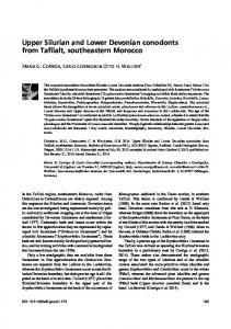
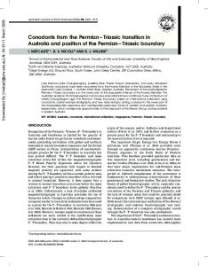
Figure 4. A, Recurrence plot of conodont abundance: Vilkaviškis-134 core (m p 3, t p 9 m, ε p 0:6j); B, AR(1) model for the Vilkaviškis-134 data (m p 3, t p 4 m, ε p 0:6j); C, Ledai-179 core (m p 3, t p 8:5 m, ε p 0:6j); D, AR(1) model for the Ledai-179 core data (m p 3, t p 4 m, ε p 0:6j). In A and C the sharp transition in recurrence rate is evident slightly before the end of the lundgreni zone. No such transitions are evident in the randomized time series B and D.
sions (Shaw 1964; Edwards 1989, 1984; Sadler 2004; Klapper and Kirchgasser 2016). The difference in terminology used here is mostly semantic, since it stems from the fact that during search for the LOC we are performing a correlation exercise in the statistical sense of optimizing the shape of the curve, based on a scatter of data points and predefined penalty function. On the other hand, the LOS search is performed by the nonstatistical pattern-tracking procedure outlined above. The purpose of both types of analysis (LOS and LOC) search is essentially the same, however, i.e., to find the best curve that can be used in rescaling the positions of events in one section into those on another section. Since in cross recurrence plots time progresses monotonically, from left to right and to the top of the plot, any regression technique should obey these pattern constraints. Thus, for the purpose of estimation of the LOC, I used so-called isotonic regression,
which satisfies these conditions (monotonic positive or nonnegative increase). Isotonic regression based on the generalized pool-adjusted-violators algorithm was implemented using package “isotone” (Mair et al. 2009) in the R statistical computation environment (R Development Core Team 2015).
Recurrence Patterns of Conodont Abundance The recurrence plot analysis of conodont abundance reveals strikingly coherent patterns (fig. 4A, 4C). In the uppermost part of the lundgreni graptolite zone, at a depth of approximately 750 m in the Vilkaviškis134 core and 658 m in the Ledai-179 core, there is a sharp increase in the recurrence rate and a transition to an irregular checkerboard-like pattern. This recurrence plot typology indicates the start of lowamplitude, quasi-regular, highly autocorrelated oscil-
Journal of Geology
CONODONT ABUNDANCE DURING THE MULDE EVENT
389
Figure 5. A, Time series of conodont abundances in the Vilkaviškis-134 section; B, moving-window analysis of recurrence rates in the recurrence plots of conodont abundance from the Vilkaviškis-134 core and 10 AR(1) randomized time series; C, time series of conodont abundances in the Ledai-134 section; D, moving-window analysis of recurrence rates in the recurrence plots of conodont abundance from the Ledai-134 section and 10 AR(1) randomized time series (m p 3, t p 9 m, ε p 0:6j). All time series were equally zero padded at their ends. Note that the recurrence rate suddenly increases in the uppermost lundgreni biozone and exceeds noise levels for the duration of the Mulde event. This implies transition from more stochastic (multifactorial) to more deterministic (governed by fever factors) dynamics.
lations. The visual comparison with the original time series of abundance dynamics (fig. 1B, 1C) shows that there is a transition in the long-term mean and also a decrease in variance and an increase in smoothness (autocorrelation) of the abundance fluctuations. The recurrence plot of both sections shows more abundant long vertical and horizontal lines in the Mulde interval, which indicates that this interval was characterized by episodes of laminar (slowly changing) states. The parallel diagonal lines are relatively short (usually of few points), though longer than in the lower part of the section in which most of the recurrence points are isolated from each other. On the other hand, distinct checkerboard patterns in the Vilkaviškis-134 record show zigzagging lines that combine individual oscillations. This indicates that the oscillations have period lengths that slightly vary over stratigraphical depth. Those variations most probably arose as a consequence of two factors. One factor is the nonlinearity of response of conodont abundances to the driving mechanisms. The sharp transition in the fluctuation pattern at the end of Jaagarahu is a clear indication of the presence of nonlinear forcing and possibly chaos. Another
factor is small-scale stochastic variations in sedimentation rate, which should be expected based on our knowledge of the time scaling of sediment accumulation, erosion, and preservation rates (Sadler 1981). The null models (fig. 4B, 4D) of the studied sections do not show any of the described patterns, only random clusters of isolated recurrence points. This indicates that the revealed patterns are not a simple result of time-invariant, autocorrelated stochastic variability. Qualitatively, the same results could be seen in comparing moving-window analyses of recurrence rates for the original signals and assemblages of randomized and autocorrelated AR(1) sequences (fig. 5). The Mulde interval is characterized by much higher recurrence rates than the pre-Mulde interval, and this difference, as is demonstrated, cannot be explained by random variations of an autocorrelated process. The cross recurrence plot between the Vilkaviškis134 and Ledai-179 sections shows a zone of increased cross recurrence starting precisely at the expected points based on the separate recurrence plot (autorecurrence) analyses, slightly below (earlier) than the Mulde intervals of both sections (fig. 6A). Therefore,
390
A. SPIRIDONOV
this study concurs with the suggestion of Loydell (2007) that conodont community collapse occurred slightly earlier than the positive carbon isotopic excursion and the “Big Crisis” of graptolites. The cross recurrence plot between the Vilkaviškis-134 and Widowo IG-1 sections, as was expected based on integrated stratigraphy, shows the highest recurrence throughout the Mulde interval (fig. 6B). In order to co-recur, the fluctuations should simultaneously have similar shapes as well as scales. Therefore, conodont abundances evolved in a very similar fashion in all three geographical areas of the eastern Baltic basin. The phase space reconstruction (fig. 7A, 7B), which revealsshapes oforbits of abundance dynamics,shows that there is sharp separation in long-term dynamics between the upper Jaagarahu and the lower Gėluva (Mulde event). The dynamics of pre-Mulde conodonts occur in the higher-abundance portion of the state spaces (top and right). In contrast, the dynamics of the Mulde conodonts occur at the intermediate- to low-abundance portions of the state space. A very similar pattern, with the exception of a couple of short-lived abundance excursions, could be seen in the Polish record (fig. 7C). Although conodont abundances in the Mulde interval sometimes achieved values as high as in the pre-Mulde interval, they soon (time lag t) return to low values. This explains the separation and indicates that the conodont abundance change in these intervals represents two different dynamical states. The search for the LOS in the cross recurrence plot between Vilkaviškis-134 and Ledai-179 cores shows moderate success in intercepting the beginning of the Mulde interval (fig. 8A): the line passes approximately 25 m below the beginning of the Mulde interval in both sections. On the other hand, the isotonic regression between these two cores is more consistent with the integrated stratigraphical model of the two successions (fig. 8B)—the LOC passes closer to the beginning of the Mulde interval by 10 m than the LOS. Figure 6. A, Cross recurrence plot of conodont abundance between the Vilkaviškis-134 and Ledai-179 sections. The increase in cross recurrence in both sections is observed slightly before the onset of the Mulde event. B, Cross recurrence plot of conodont abundance change between the Vilkaviškis-134 and Widowo IG-1 sections (m p 3, t p 9 m, ε p 0:6j). The increase in cross recurrence in Vilkaviškis-134 starts slightly before the end of the lundgreni biozone. The whole studied Widowo IG-1 interval is characterized by increased cross recurrence with the upper part of the Vilkaviškis-134 section. This implies that in the Widowo IG-1 core we see only the Mulde interval.
Implications for Evolutionary Paleoecology The coherent patterns described here reveal a marked difference between the dynamical states of the lower and upper parts of the Homerian stage. The dynamical transition in the uppermost part of the lundgreni biozone was marked by a long-term decrease in abundances, as well as a transition to more orderly and steady dynamics with rare abundance excursions (fig. 7C). The observed dynamics of the Mulde interval fit well with a category of bioevent recently termed a “mass rarity” (Hull et al. 2015), where a
Journal of Geology
CONODONT ABUNDANCE DURING THE MULDE EVENT
Figure 7. Phase space reconstruction of conodont abundance dynamics in the first two embedding dimensions (m p 2, t p 9 m). A, Vilkaviškis-134; B, Ledai-179; C, Widowo IG-1. Here, interpolated (with 0.5-m rate) values were used. The last 9 m of each section was omitted due to the constraints imposed by the time series embedding. Rhombuses indicate states from the pre-Mulde interval. Triangles indicate states of the Mulde interval, with the transitionary data points (a(t)Jaagarahu, a(t1t)Gėluva) also as-
391
global disturbance leads to low abundance and low local diversity, as is recognized for this event (Jeppsson 1998; Radzevičius et al. 2014, 2016), with altered ecological interactions. The decrease in volatility of abundance dynamics, the increase in recurrence rate, and the increase in number and lengths of vertical, horizontal, and, to a lesser extent, diagonal lines on the recurrence plots indicate that the shift was a transition from higher dimensional to lower dimensional, though not ideally cyclic dynamics (e.g., stochasticity ⇒ chaos transition). This accords with Jeppsson’s conjecture that the Mulde event proceeded through a series of (quasi-)periodic disturbances or datum planes. The transition to the quasi-periodic fluctuation regime would result in an increase in recurrence rates and a general increase in autocorrelation, which is evident in the recurrence and cross recurrence analyses presented here. It could be argued that the observed change between pre-Mulde and Mulde intervals is a direct reflection of the changes in sedimentary environments, since mid- to upper Homerian times apparently experienced more volatile sea level changes than did the lower Homerian (Calner and Jeppsson 2003; Cramer et al. 2006, 2011; Radzevičius et al. 2014a, forthcoming). Application of sequence stratigraphy to biostratigraphy has transformed our understanding of apparent paleoecological and evolutionary patterns in the fossil record (Brett 1995; Holland 1995; Patzkowsky and Holland 2012). Sea level change predictably affects the apparent abundance of fossils through changes in sediment supply, exhaustion, and creation of sediment accommodation space and changes in preservation potential due to predictably changing hydrodynamic, biogeochemical, and bioerosional regimes (Brett and Baird 1986; McGoff 1991; Brett 1995; Catuneanu 2006; Tomašových and Schlögl 2008; Tomašových and Kidwell 2010; Vierek and Racki 2011; Jarochowska et al. 2016).There are strongindications,however, that even hydrodynamically active environments may reliably preserve community compositions, including those of conodonts (Tomašových 2006; Vierek and Racki 2011). What these models and observations predict is that, in general, increased environmental volatility and proximity to the shoreline should increase the range and frequency of fluctuations in abundance, because near-shore environments experience more signed to the Mulde interval. The clear separation between pre-Mulde and Mulde dynamics (A, B) can be observed. The whole Widowo IG-1 section (C) presumably falls into the Mulde interval (Jarochowska and Munnecke 2015). Note that the systems’ orbits unfold unimodaly, at the lower left corner of the graph.
392
A. SPIRIDONOV
Figure 8. A, Estimation of the line of synchronization in the cross recurrence plots of the Vilkaviškis-134 and Ledai179 sections by searching for the most consistent diagonal-like line recurrence, using the method described in Marwan et al. (2007; m p 3, t p 9 m, ε p 0:6j). B, Estimation of the line of correlation (LOC) in the same cross recurrence plot data converted to the cross plot using isotonic regression. From the graphs it can be seen that the LOC produced by the isotonic regression shows a closer match to the expectation; i.e., it is closer to the intersection point of Mulde intervals in both sections.
diverse and intercorrelated disturbing factors. Moreover, the nearshore environment has a greater propensity to generate diastems and unconformities, which bring into closer proximity abundance values that are more widely separated in time, i.e., increased “jumpiness” in the abundance record. Exactly this pattern was observed in the Baltic record of Pridoli conodonts (Spiridonov et al. 2016). The conodont abundance time series from the more nearshore facies belt exhibited increased spectral “whitening” and volatility of abundance dynamics; i.e., abundance change was less autocorrelated than in deeper environments. On the other hand, here we observe the opposite pattern. Volatility was much higher and therefore recurrence was much lower in the lower part of the section, which represents environmentally much more stable intervals from relatively deeper environments. The Mulde interval and uppermost Jaagarahu time, where most of the large sea level changes and other perturbations occurred, show much more deterministic, quasi-periodic oscillations, indicating increased autocorrelation. Moreover, the whole Gėluva time was characterized by two long fourth-order (≈20-m or approximately 400-kalong) sedimentary cycles, which are attributed to sea level change (Radzevičius et al. 2014a, forthcoming), and the conodont abundance record (fig. 1B, 1C) was dominated by higher-frequency (fifth- to sixth-order) fluctuations (tens of thousands up to a couple hundred thousand years in duration or, if calculating in stratigraphic thickness at given localities, 7–8- to 1.5-m-long oscillations). Therefore, it can be con-
cluded that the observed patterns of change in conodont abundance dynamics were not dominated by the passive physical structuring of stratigraphical record but in large part represent a genuinely primary paleoecological signal. Abundant work on the mid-Homerian bioevent shows that the main cause of biotic perturbations was a drop in temperature and changes in oceanographic conditions (Radzevičius et al. 2016; Trotter et al. 2016). If the long-term global climatic disturbance was the ultimate cause of the Mulde and lundgreni events, then, based on the deductions of dynamical systems theory and the evidence presented here, we are witnessing a so-called classical critical (or catastrophic) phase transition driven by external factors (Scheffer and Carpenter 2003; Pascual and Guichard 2005). One of the most likely proximate mechanisms of depletion and structural changes in the paleocommunities is a bottom-up disruption and sequential collapse of food webs (Roopnarine 2009). Given the recent evidence on the compositional and diversity dynamics of phytoplankton, the collapse of the primary production during the Mulde event is very unlikely (Venckutė-Aleksienė et al. 2016). However, the possibility of a collapse starting from the lower heterotrophic levels is a plausible explanation. Critical phase transitions in ecosystems are usually a result of the sequential collapses of many dependent components, with multiple interacting regime shifts (Brock and Carpenter 2010) progressing toward the final loss of resilience of the interaction network (Gao
Journal of Geology
CONODONT ABUNDANCE DURING THE MULDE EVENT
et al. 2016). Therefore, the causality of the Mulde transition and its extent could be determined by analyzing and comparing the high-resolution abundance time series of other significant ecological guilds and taxa. The approach outlined here could be used in studying systemic dynamical changes in communities that occur during other so-called mass rarity events, and the future (i.e., “Anthropocene”; Waters et al. 2014) ocean ecosystems probably will experience similar events (or biosphere states; Hull et al. 2015). Implications for Quantitative Biostratigraphy Phylogenetic autocorrelation—a similarity in the behavior and structure of taxa due to recent common ancestry—usually causes problems in macroevolutionary studies (Raup et al. 1973). Here, however, it helps illuminate the impact of large-scale disturbances in environments dominated by differing but closely related species through the study of their abundance proxies. Abundance events (acme zones or epiboles), which are extensively used in ecostratigraphy and sequence stratigraphy (Waterhouse 1976; Urbanek 1993; Brett 1995; Sageman et al. 1997), have been criticized for their low consistency and inaccuracy (Sadler 2004). On the other hand, the treatment of temporal abundance information as a mathematical “flow” or “map” uses all the information embedded in a time series. Time-evolutive approaches, using spectral theory (e.g., Spiridonov et al. 2016), as well as those based on nonlinear dynamics theory presented here, help to distinguish the dynamical differences of so-called primo- and secundo-oceanic episodes (Jeppsson 1998) and transitions (events) between them. Traditional biostratigraphic events—the first and last appearances of species—are treated as unique, and rightly so, due to the contingency of evolution (Gould 1990, 2001) and the irreversibility and imminence of extinction (Raup 1994). On the other hand, quantitative (including abundance) or categorical information is usually treated as nonunique (Edwards 1989; Miall 2010) and thus significantly inferior for stratigraphic problem solving. Here I will demonstrate that this is too pessimistic, even for short time series, given realistic data constraints. Separate states may be repeated frequently, but repetition of their configurations is very unlikely. Suppose at each sample point the abundance a(ti) of conodont elements per kilogram of rock could achieve any value ranging from 1 to 1000 (similar to the range observed in this contribution) and we have very short time series of 10 samples in length, then, according to the laws of probability, any given configuration will have probability equal to the size of
393
possibility space (number of discrete states) raised to the negative power of the time series length: 210 P(a(t10 )ja(t9 ), :::, a(t1 )) p (103 ) p 10230 . And if we assume that this fluctuation pattern is spatially nonlocal, then we should expect unique (highly improbable) and correlatable sequences. This example shows that even if our long and spatiotemporally coherent pattern is distorted by sedimentation breaks (i.e., shredded to some degree; Sadler 1981; Jerolmack and Paola 2010), the smaller portions of it, as small as several samples, would still preserve sufficient amounts of unique information. Because those portions would additionally preserve their temporal order (i.e., rank), cross recurrence plots would detect these correlatable episodes (see fig. 9A for a model demonstration). Furthermore, if we imagine another situation where we have two mostly stochastic and idiosyncratic abundance signals that show intermittent short-term similarity (spatial coherence), we would still retrieve the information from cross recurrence plots and be able to correlate the sequences using appropriate regression techniques (model of “islands of determinism in the stochastic sea” in fig. 9B). Exactly these combinatorial properties of informationally similar sequences are used in the bioinformatics of nucleic acid alignment and especially so in studies of ancient DNA that often analyze fragmented to very short pieces (Li and Durbin 2009; Prüfer et al. 2010). Short, separate fragments do not preclude fairly complete reconstruction of ancient species genomes (Miller et al. 2008; Prüfer et al. 2014), proving the possibility of using fragmented and noisy sequences for reconstructing long, extremely complex patterns. Stratigraphy, on the other hand, has two advantages in reconstructing spatially distributed congruent sequences of abundance fluctuations. First, as already mentioned, the order of sequences is preserved (if tectonically undisturbed). Second, the information coding capacity (number of states) of abundance values is many orders of magnitude higher than in nucleotide analyses (exactly this property, sometimes, allows the use of even singular abundance peaks for the correlation). The major difficulty for the use of quantitative information in stratigraphic correlation lies in the search for reliable and broadly applicable variables in spatial and temporal domains. The abundance of conodont elements could be one of the best variables in this respect. Conodonts were widely distributed in marine environments. They had relatively narrow ecology (in comparison to bony fishes, e.g.). The number of elements in conodont apparatuses is broadly comparable, and the elements are very resistant to diagenesis. These qualities make them potentially better proxies for long-distance
394
A. SPIRIDONOV
Figure 9. A, Cross recurrence plot of zero-padded conodont abundance time series of the Vilkaviškis-134 core against its decimated version (decimation at points in the interpolated sample time t ∈ [11; 20], [51; 60], [101; 110], and [151; 160]), with added uniform white noise (jnoise =jsignal p 0:1; here jnoise is the standard deviation of the white noise and jsignal is the standard deviation of the original conodont abundance time series). Recurrence plot embedding and filtering parameters are the same as in figure 5. Note that the addition of four hiatuses, which constitute approximately 22% of the time series duration, and moderate levels of added noise were insufficient to preclude distinguishing dynamical transitions and synchronizing the two records. B, Cross recurrence plot of two zero-padded white noise time series with three intermittent episodes of common periodic fluctuations (m p 3, t p 2, ε p 0:3j). The two time series (ts1 and ts2) are essentially different, except for the three short identical episodes of periodic deterministic fluctuations. Those episodes are sufficient to reveal the long-term temporal connection between the time series.
synchronization than geophysical logs and most of the geochemical proxies, which can be highly compromised by postdepositional processes that degrade primary values. The comparison between very different facies, however (especially in condensed sections such as south-central Oklahoma, where conodont abundances in the upper Mulde interval are much higher than reported here; Barrick et al. 2009), will need further abundance normalization by dividing compared time series by their average (or running average) values or by the maximum values. This study reveals great potential for the use of conodont abundance trends in high-resolution stratigraphy, if completed with care and with appropriate mathematical machinery. The differing dynamic
patterns described here occur at levels that other stratigraphic evidence (conodont, graptolite, and d13C stratigraphy) show to be coeval, despite some regional differences in taxonomic composition, sedimentation, and sampling. In correlation experiments, the LOS search algorithm synchronized the time series less accurately than isotonic LOC regression, though the major matches were detected by both approaches. Further testing with diverse dynamical structures and optimization techniques is needed in order to determine the best approaches for various dynamical patterns, i.e., highly synchronized and continuous as opposed to episodically coupled and thus disjunct as reported in this study.
Journal of Geology
CONODONT ABUNDANCE DURING THE MULDE EVENT
Conclusions. Recurrence and cross recurrence analyses of conodont abundance records from the eastern part of the Silurian Baltic basin reveal congruent patterns of change in dynamical regime that started slightly before the lundgreni graptolite event and the start of Mulde stable carbon isotopic anomaly. Fluctuations in conodont abundance show more ordered structure in the uppermost Jaagarahu and Gėluva regional stages than in the middle part of the Jaagarahu. This implies the presence of quasi-periodic oscillations in the upper part of the sections. The transition is coincidental with the conodont evolutionary turnover event and the decrease in conodont diversity (e.g., Jeppsson 1998; Radzevičius et al. 2014). The evidence supports Jepson’s model of synchronous, widespread, and quasi-periodic perturbations of conodont communities during oceanic events. Moreover, the recognition of these coherent dynamic patterns does not demand the large sample sizes that are needed to retrieve rare taxa. Clear separation of dynamics in the reconstructed phase space and the striking differences in the recurrence plots indicate that mid-Homerian conodont communities experienced a critical transition in their community dynamics that can be traced at least at a regional scale. Coherent spatial and temporal patterns in fluctuating conodont abundance, in combination with the cross recurrence analyses, reveal their potential for correlating stratigraphic sections. The correlation of sections, based on isotonic regression using cross recurrence matrices, shows higher accuracy than the LOS search algorithm as implemented in the CRP Toolbox. Further experiments with diverse
395
dynamical structures and algorithms are needed in order to find optimal stratigraphic correlation strategies using cross recurrence plots. The results of recurrence plot analysis already reveal that conodont abundances are surprisingly resilient to moderate levels of noise and data degradation. Assuming realistic data constraints, even episodic and short-term spatiotemporal coherence in the abundance dynamics can be used for reliable correlation of geological sections, as justified by the laws of conditional probability. Stratigraphic correlation of abundance data on cross recurrence plots can be used as a potentially continuous complement to high-resolution event stratigraphy (Cramer et al. 2015), ultimately raising resolving power in a broad range of environments.
ACKNOWLEDGMENTS
Many thanks go to P. Sadler (University of California, Riverside), M. Foote (University of Chicago), and an anonymous colleague for encouraging criticism, many helpful suggestions, and valuable references that strengthened and clarified the manuscript. I would also like to acknowledge A. Brazauskas for consultations on taxonomy and S. Radzevičius for his opinions on stratigraphy. This research was sponsored by a Lithuanian Academy of Sciences grant for young scientists. The publication of the article was funded by the Research Council of Lithuania. This is a contribution to IGCP 591: “The Early to Middle Paleozoic Revolution” and “Event Stratigraphy in the Silurian Sedimentary Basin of Lithuania.”
REFERENCES CITED
Aldridge, R. J.; Jeppsson, L.; and Dorning, K. J. 1993. Early Silurian oceanic episodes and events. J. Geol. Soc. Lond. 150:501–513. Bambach, R. K. 2006. Phanerozoic biodiversity mass extinctions. Annu. Rev. Earth Planet. Sci. 34:127–155. Barrick, J. E.; Kleffner, M. A.; and Karlsson, H. R. 2009. Conodont faunas and stable isotopes across the Mulde event (late Wenlock; Silurian) in southwestern Laurentia (south-central Oklahoma and subsurface west Texas). In D. J. Over, ed. Conodont studies commemorating the 150th anniversary of the first conodont paper (Pander, 1856) and the 40th anniversary of the Pander Society. Ithaca, NY, Paleontological Research Institution. Brett, C. E. 1995. Sequence stratigraphy, biostratigraphy, and taphonomy in shallow marine environments. Palaios 10:597–616. Brett, C. E., and Baird, G. C. 1986. Comparative taphonomy: a key to paleoenvironmental interpretation based on fossil preservation. Palaios 1:207–227.
Brock, W. A., and Carpenter, S. R. 2010. Interacting regime shifts in ecosystems: implication for early warnings. Ecol. Monogr. 80:353–367. Calner, M. 2008. Silurian global events: at the tipping point of climate change. In A. Elewa, ed. Mass extinction. Berlin, Springer, p. 21–57. Calner, M., and Jeppsson, L. 2003. Carbonate platform evolution and conodont stratigraphy during the middle Silurian Mulde Event, Gotland, Sweden. Geol. Mag. 140:173–203. Catuneanu, O. 2006. Principles of sequence stratigraphy. Amsterdam, Elsevier. Chelidze, T., and Matcharashvili, T. 2015. Dynamical patterns in seismology. In Webber, C. L., Jr., and Marwan, N., eds. Recurrence quantification analysis. Amsterdam, Springer, p. 291–334. Cooper, R. A.; Sadler, P. M.; Munnecke, A.; and Crampton, J. S. 2014. Graptoloid evolutionary rates track Ordovician-Silurian global climate change. Geol. Mag. 151:349–364.
396
A. SPIRIDONOV
Cramer, B. D.; Brett, C. E.; Melchin, M. J.; Maennik, P.; Kleffner, M. A.; McLaughlin, P. I.; Loydell, D. K.; et al. 2011. Revised correlation of Silurian Provincial Series of North America with global and regional chronostratigraphic units and d13Ccarb chemostratigraphy. Lethaia 44:185–202. Cramer, B. D.; Kleffner, M. A.; and Saltzman, M. R. 2006. The late Wenlock Mulde positive carbon isotope (d13Ccarb) excursion in North America. GFF 128:85–90. Cramer, B. D.; Vandenbroucke, T. R. A.; and Ludvigson, G. A. 2015. High-resolution event stratigraphy (HiRES) and the quantification of stratigraphic uncertainty: Silurian examples of the quest for precision in stratigraphy. Earth-Sci. Rev. 141:136–153. Crampton, J. S.; Cooper, R. A.; Sadler, P. M.; and Foote, M. 2016. Greenhouse-icehouse transition in the Late Ordovician marks a step change in extinction regime in the marine plankton. Proc. Natl. Acad. Sci. USA 113: 1498–1503. Donoghue, P. C. J., and Purnell, M. A. 1999. Growth, function, and the conodont fossil record. Geology 27: 251–254. Dzik, J. 2016. Evolutionary roots of the conodonts with increased number of elements in the apparatus. Earth Environ. Sci. Trans. R. Soc. Edinb. 106:29–53. Eckmann, J.-P.; Kamphorst, S. O.; and Ruelle, D. 1987. Recurrence plots of dynamical systems. Europhys. Lett. 4:973–977. Edwards, L. E. 1984. Insights on why graphic correlation (Shaw’s method) works. J. Geol. 92:583–597. ———. 1989. Supplemented graphic correlation: a powerful tool for paleontologists and nonpaleontologists. Palaios 4:127–143. Einasto, P. E.; Abushik, A. F.; Kaljo, D. L.; Koren, T. N.; Modzalevskaya, T. L.; Nestor, N. E.; and Klaamann, E. 1986. Osobiennosti silurskogo osadkonakopleniya i associacii fauny v kraevych basseinach Pribaltiki i Podolii. In Kaljo, D. L., and Klaamann, E., eds. Teoria i opyt ekostratigrafii. Tallin, Valgus, p. 65–72. Fabretti, A., and Ausloos, M. 2005. Recurrence plot and recurrence quantification analysis techniques for detecting a critical regime: examples from financial market inidices. Int. J. Mod. Phys. C 16:671–706. Foote, M. 2005. Pulsed origination and extinction in the marine realm. Paleobiology 40:6–20. Gao, J.; Barzel, B.; and Barabási, A.-L. 2016. Universal resilience patterns in complex networks. Nature 530: 307–312. Girard, C., and Renaud, S. 2007. Quantitative conodontbased approaches for correlation of the Late Devonian Kellwasser anoxic events. Palaeogeogr. Palaeoclimatol. Palaeoecol. 250:114–125. Gould, S. J. 1990. Wonderful life: the Burgess Shale and the nature of history. New York, Norton. ———. 2001. Contingency. In Briggs, D. E. G., and Crowther, P. R., eds. Palaeobiology II. Malden, MA, Blackwell Science, p. 195–198. doi:10.1002/9780470999295.ch41. Hegger, R.; Kantz, H.; and Schreiber, T. 1999. Practical implementation of nonlinear time series methods: the TISEAN package. Chaos 9:413–435.
Herrmann, A. D.; Barrick, J. E.; and Algeo, T. J. 2015. The relationship of conodont biofacies to spatially variable water mass properties in the Late Pennsylvanian Midcontinent Sea. Paleoceanography 30:269–283. Holland, S. M. 1995. The stratigraphic distribution of fossils. Paleobiology 21:92–109. Hull, P. M.; Darroch, S. A. F.; and Erwin, D. H. 2015. Rarity in mass extinctions and the future of ecosystems. Nature 528:345–351. Jarochowska, E.; Bremer, O.; Heidlas, D.; Pröpster, S.; Vandenbroucke, T. R. A.; and Munnecke, A. 2016. EndWenlock terminal Mulde carbon isotope excursion in Gotland, Sweden: integration of stratigraphy and taphonomy for correlations across restricted facies and specialized faunas. Palaeogeogr. Palaeoclimatol. Palaeoecol. 457:304–322. Jarochowska, E., and Munnecke, A. 2015. Late Wenlock carbon isotope excursions and associated conodont fauna in the Podlasie Depression, eastern Poland: a not-so-big crisis? Geol. J. 51:683–703. Jarochowska, E.; Munnecke, A.; Frisch, K.; Ray, D. C.; and Castagner, A. 2015. Faunal and facies changes through the mid Homerian (late Wenlock, Silurian) positive carbon isotope excursion in Podolia, western Ukraine. Lethaia 49:170–198. Jeppsson, L. 1987. Lithological and conodont distributional evidence for episodes of anomalous oceanic conditions during the Silurian. In Aldridge, R. J., ed. Palaeobiology of conodonts. Chichester, Horwood, p. 129–145. ———. 1997. The anatomy of the mid-early Silurian Ireviken Event and a scenario for PS events. In Brett, C. E., and Baird, G. C., eds. Paleontological events: stratigraphic, ecological, and evolutionary implications. New York, Columbia University Press, p. 451–492. ———. 1998. Silurian oceanic events: summary of general characteristics. In Landing, E., and Johnson, M. E., eds. Silurian cycles: linkages of dynamic stratigraphy with atmospheric, oceanic and tectonic changes. New York, New York State Museum, p. 237–257. Jeppsson, L., and Calner, M. 2002. The Silurian Mulde Event and a scenario for secundo-secundo events. Earth Environ. Sci. Trans. R. Soc. Edinb. 93:135–154. Jeppsson, L., and Männik, P. 1993. High-resolution correlations between Gotland and Estonia near the base of the Wenlock. Terra Nova 5:348–358. Jerolmack, D. J., and Paola, C. 2010. Shredding of environmental signals by sediment transport. Geophys. Res. Lett. 37. doi:10.1029/2010GL044638. Kantz, H., and Schreiber, T. 2004. Nonlinear time series analysis. Vol. 7. Cambridge, Cambridge University Press. Kirkpatrick, M. 2010. Rates of adaptation: why is Darwin’s machine so slow? In Bell, M. A.; Futuyma, D. J.; Eanes W. F.; and Levinton, J. W., eds. Evolution since Darwin: the first 150 years. Sunderland, MA, Sinauer, p. 177–195. Klapper, G., and Kirchgasser, W. T. 2016. Frasnian Late Devonian conodont biostratigraphy in New York: graphic correlation and taxonomy. J. Paleontol. 90: 525–554.
Journal of Geology
CONODONT ABUNDANCE DURING THE MULDE EVENT
Lenton, T. M.; Dahl, T. W.; Daines, S. J.; Mills, B. J. W.; Ozaki, K.; Saltzman, M. R.; and Porada, P. 2016. Earliest land plants created modern levels of atmospheric oxygen. Proc. Natl. Acad. Sci. USA 113:9704–9709. Li, H., and Durbin, R. 2009. Fast and accurate short read alignment with Burrows-Wheeler transform. Bioinformatics 25:1754–1760. Loydell, D. K. 2007. Early Silurian positive d13C excursions and their relationship to glaciations, sea-level changes and extinction events. Geol. J. 42:531–546. Mair, P.; Hornik, K.; and de Leeuw, J. 2009. Isotone optimization in R: pool-adjacent-violators algorithm (PAVA) and active set methods. J. Stat. Softw. 32:1–24. Martma, T.; Brazauskas, A.; Kaljo, D.; Kaminskas, D.; and Musteikis, P. 2005. The Wenlock-Ludlow carbon isotope trend in the Vidukle core, Lithuania, and its relations with oceanic events. Geol. Q. 49:223–234. Marwan, N. 2011. How to avoid potential pitfalls in recurrence plot based data analysis. Int. J. Bifurc. Chaos 21:1003–1017. Marwan, N., and Kurths, J. 2002. Nonlinear analysis of bivariate data with cross recurrence plots. Phys. Lett. A 302:299–307. Marwan, N.; Romano, M. C.; Thiel, M.; and Kurths, J. 2007. Recurrence plots for the analysis of complex systems. Phys. Rep. 438:237–329. Marwan, N.; Thiel, M.; and Nowaczyk, N. R. 2002. Cross recurrence plot based synchronization of time series. Nonlinear Proc. Geophys. 9:325–331. Marwan, N., and Webber, C. L., Jr. 2015. Mathematical and computational foundations of recurrence quantifications. In Webber, C. L., Jr., and Marwan, N., eds. Recurrence quantification analysis. New York, Springer, p. 3–43. McGoff, H. J. 1991. The hydrodynamics of conodont elements. Lethaia 24:235–247. Melchin, M. J.; Koren, T. N.; and Štorch, P. 1998. Global diversity and survivorship patterns of Silurian graptoloids. In Landing, E., and Johnson, M, eds. Silurian cycles. Albany, New York State Museum, p. 165–182. Miall, A. D. 2010. The geology of stratigraphic sequences. 2nd ed. Berlin, Springer. Miller, W.; Drautz, D. I.; Ratan, A.; Pusey, B.; Qi, J.; Lesk, A. M.; Tomsho, L. P.; Packard, M. D.; Zhao, F.; and Sher, A. 2008. Sequencing the nuclear genome of the extinct woolly mammoth. Nature 456:387–390. Molloy, P. D., and Simpson, A. J. 2012. An analysis of the Ireviken Event in the Boree Creek Formation, New South Wales, Australia. In Talent, J., ed. Earth and life. Heidelberg, Springer, p. 615–630. Nicolis, C., and Nicolis, G. 1986. Reconstruction of the dynamics of the climatic system from time-series data. Proc. Natl. Acad. Sci. USA 83:536–540. Pascual, M., and Guichard, F. 2005. Criticality and disturbance in spatial ecological systems. Trends Ecol. Evol. 20:88–95. Patzkowsky, M. E., and Holland, S. M. 2012. Stratigraphic paleobiology: understanding the distribution of fossil taxa in time and space. Chicago, University of Chicago Press.
397
Prüfer, K.; Racimo, F.; Patterson, N.; Jay, F.; Sankararaman, S.; Sawyer, S.; Heinze, A.; Renaud, G.; Sudmant, P. H.; and De Filippo, C. 2014. The complete genome sequence of a Neanderthal from the Altai Mountains. Nature 505:43–49. Prüfer, K.; Stenzel, U.; Hofreiter, M.; Pääbo, S.; Kelso, J.; and Green, R. E. 2010. Computational challenges in the analysis of ancient DNA. Genome Biol. 11:1. Purnell, M. A., and Donoghue, P. C. 2005. Between death and data: biases in interpretation of the fossil record of conodonts. Spec. Pap. Palaeontol. 73:7–25. R Development Core Team. 2015. R: a language and environment for statistical computing. Version 3.1.3. Vienna, R Foundation for Statistical Computing. Radzevičius, S. 2006. Late Wenlock biostratigraphy and the Pristiograptus virbalensis group (Graptolithina) in Lithuania and the Holy Cross Mountains. Geol. Q. 50:333–344. Radzevičius, S.; Spiridonov, A.; and Brazauskas, A. 2014a. Application of wavelets to the cyclostratigraphy of the Upper Homerian (Silurian) Gėluva Regional Stage in the Viduklė-61 Deep Well (western Lithuania). In Pais, J., ed. STRATI 2013. Berlin, Springer. doi:10.1007 /978-3-319-04364-7_84. ———. 2014b. Integrated middle-upper Homerian (Silurian) stratigraphy of the Viduklė-61 well, Lithuania. GFF 136:218–222. Radzevičius, S.; Spiridonov, A.; Brazauskas, A.; Dankina, D.; Rimkus, A.; Bičkauskas, G.; Kaminskas, D.; Meidla, T.; and Ainsaar, L. 2016. Integrated stratigraphy, conodont turnover and paleoenvironments of the Upper Wenlock and Ludlow of the Vilkaviškis-134 core (Lithuania). Newsl. Stratigr. 49:321–336. Radzevičius, S.; Spiridonov, A.; Brazauskas, A.; Norkus, A.; Meidla, T.; and Ainsaar, L. 2014. Upper Wenlock d13C chemostratigraphy, conodont biostratigraphy and palaeoecological dynamics in the Ledai-179 drill core (eastern Lithuania). Estonian J. Earth Sci. 63:293–299. Radzevičius, S.; Tumakovaitė, B.; and Spiridonov, A. Forthcoming. Upper Homerian (Silurian) high-resolution correlation using cyclostratigraphy: an example from western Lithuania. Acta Geol. Pol. Raup, D. M. 1994. The role of extinction in evolution. Proc. Natl. Acad. Sci. USA 91:6758–6763. Raup, D. M.; Gould, S. J.; Schopf, T. J. M.; and Simberloff, D. S. 1973. Stochastic models of phylogeny and the evolution of diversity. J. Geol. 81:525–542. Raup, D. M., and Sepkoski, J. J. 1982. Mass extinctions in the marine fossil record. Science 215:1501–1503. Roopnarine, P. D. 2009. Ecological modeling of paleocommunity food webs. Paleontol. Soc. Pap. 15:195–220. Rosenstein, M. T.; Collins, J. J.; and De Luca, C. J. 1993. A practical method for calculating largest Lyapunov exponents from small data sets. Physica D 65:117–134. Sadler, P. M. 1981. Sediment accumulation rates and the completeness of stratigraphic sections. J. Geol. 89:569– 584. ———. 2004. Quantitative biostratigraphy: achieving finer resolution in global correlation. Annu. Rev. Earth Planet. Sci. 32:187–213.
398
A. SPIRIDONOV
———. 2012. Integrating carbon isotope excursions into automated stratigraphic correlation: an example from the Silurian of Baltica. Bull. Geosci. 87:681–694. Sageman, B. B.; Kauffman, E. G.; Harries, P. J.; and Elder, W. P. 1997. Cenomanian/Turonian bioevents and ecostratigraphy in the Western Interior Basin: contrasting scales of local, regional, and global events. In Brett, C. E., and Baird, G. C., eds. Paleontological events: stratigraphic, ecological and evolutionary implications. New York, Columbia University Press, p. 520–570. Saltzman, M. R. 2005. Phosphorus, nitrogen, and the redox evolution of the Paleozoic oceans. Geology 33: 573–576. Samtleben, C.; Munnecke, A.; Bickert, T.; and Pätzold, J. 1996. The Silurian of Gotland (Sweden): facies interpretation based on stable isotopes in brachiopod shells. Geol. Rundsch. 85:278–292. Scheffer, M., and Carpenter, S. R. 2003. Catastrophic regime shifts in ecosystems: linking theory to observation. Trends Ecol. Evol. 18:648–656. Shaw, A. B. 1964. Time in stratigraphy. In Shrock, R. R., ed. International Series in the Earth Sciences. New York, McGraw-Hill. Sibert, E.; Norris, R.; Cuevas, J.; and Graves, L. 2016. Eighty-five million years of Pacific Ocean gyre ecosystem structure: long-term stability marked by punctuated change. Proc. R. Soc. B. 283:20160189. doi:10 .1098/rspb.2016.0189. Spiridonov, A.; Brazauskas, A.; and Radzevičius, S. 2015. The role of temporal abundance structure and habitat preferences in the survival of conodonts during the midearly Silurian Ireviken mass extinction event. PLoS ONE 10:e0124146. ———. 2016. Dynamics of abundance of the mid- to late Pridoli conodonts from the eastern part of the Silurian Baltic basin: multifractals, state shifts, and oscillations. Am. J. Sci. 316:363–400. Spiridonov, A.; Kaminskas, D.; Brazauskas, A.; and Radzevičius, S. Forthcoming. Time hierarchical analysis of conodont paleocommunities and environmental change before and during the onset of the Lower Silurian Mulde bioevent. Glob. Planet. Change. Stam, C. J. 2005. Nonlinear dynamical analysis of EEG and MEG: review of an emerging field. Clin. Neurophysiol. 116:2266–2301. Takens, F. 1981. Detecting strange attractors in turbulence. In Rand, D. A., and Young, L. S. Lecture Notes in Mathematics 898. Berlin, Springer. Tomašových, A. 2006. Linking taphonomy to communitylevel abundance: insights into compositional fidelity of the Upper Triassic shell concentrations (Eastern Alps). Palaeogeogr. Palaeoclimatol. Palaeoecol. 235:355– 381. Tomašových, A., and Kidwell, S. M. 2010. Predicting the effects of increasing temporal scale on species com-
position, diversity, and rank-abundance distributions. Paleobiology 36:672–695. Tomašových, A., and Schlögl, J. 2008. Analyzing variations in cephalopod abundances in shell concentrations: the combined effects of production and densitydependent cementation rates. Palaios 23:648–666. Trauth, M. H.; Bookhagen, B.; Marwan, N.; and Strecker, M. R. 2003. Multiple landslide clusters record Quaternary climate changes in the northwestern Argentine Andes. Palaeogeogr. Palaeoclimatol. Palaeoecol. 194:109–121. Trotter, J. A.; Williams, I. S.; Barnes, C. R.; Männik, P.; and Simpson, A. 2016. New conodont d18O records of Silurian climate change: implications for environmental and biological events. Palaeogeogr. Palaeoclimatol. Palaeoecol. 443:34–48. Urbanek, A. 1993. Biotic crises in the history of Upper Silurian graptoloids: a palaeobiological model. Hist. Biol. 7:29–50. Vandenbroucke, T. R. A.; Emsbo, P.; Munnecke, A.; Nuns, N.; Duponchel, L.; Lepot, K.; Quijada, M.; Paris, F.; Servais, T.; and Kiessling, W. 2015. Metal-induced malformations in early Palaeozoic plankton are harbingers of mass extinction. Nat. Commun. 6:7966. doi:10.1038/ncomms8966. Vařilová, Z.; Zvelebil, J.; and Paluš, M. 2011. Complex system approach to interpretation of monitoring time series: two case histories from NW Bohemia. Landslides 8:207–220. Venckutė-Aleksienė, A.; Radzevičius, S.; and Spiridonov, A. 2016. Dynamics of phytoplankton in relation to the upper Homerian (Lower Silurian) lundgreni event: an example from the eastern Baltic basin (western Lithuania). Mar. Micropaleontol. 126:31–41. Vierek, A., and Racki, G. 2011. Depositional versus ecological control on the conodont distribution in the Lower Frasnian fore-reef facies, Holy Cross Mountains, Poland. Palaeogeogr. Palaeoclimatol. Palaeoecol. 312:1–23. Waterhouse, J. B. 1976. The significance of ecostratigraphy and need for biostratigraphic hierarchy in stratigraphic nomenclature. Lethaia 9:317–326. Waters, C. N.; Zalasiewicz, J. A.; Williams, M.; Ellis, M. A.; and Snelling, A. M. 2014. A stratigraphical basis for the Anthropocene? Geol. Soc. Lond. Spec. Publ. 395:1–21. Webber, C. L., Jr., and Marwan, N. 2015. Recurrence quantification analysis: theory and best practices. Cham, Springer. Weedon, G. P. 2003. Time-series analysis and cyclostratigraphy: examining stratigraphic records of environmental cycles. Cambridge, Cambridge University Press. Zbilut, J. P.; Giuliani, A.; and Webber, C. L. 1998. Detecting deterministic signals in exceptionally noisy environments using cross-recurrence quantification. Phys. Lett. A 246:122–128.