IEEE 802.11b wireless access technology operating in DCF mode over ... Recently, it was shown that the frame error process of the wireless channels.
Simple, accurate and computationally efficient wireless channel modeling algorithm Dmitri Moltchanov, Yevgeni Koucheryavy, Jarmo Harju Institute of Communication Engineering, Tampere University of Technology, P.O.Box 553, Tampere, Finland {moltchan,yk,harju}@cs.tut.fi
Abstract. We propose simple and computationally efficient wireless channel modeling algorithm. For this purpose we adopt the special case of the algorithm initially proposed in [1] and show that its complexity significantly decreases when the time-series is covariance stationary binary in nature. We show that for such time-series the solution of the inverse eigenvalue problem returns unique transition probability matrix of the modulating Markov chain that is capable to match statistical properties of empirical frame error processes. Our model explicitly takes into account autocorrelational and distributional properties of empirical data. We validate our model against empirical frame error traces of IEEE 802.11b wireless access technology operating in DCF mode over spread spectrum at 2Mbps and 5.5 Mbps bit rates. We also made available the C code of the model as well as pre-compiled binaries for Linux and Windows operating systems at http://www.cs.tut.fi/˜moltchan.
1
Introduction
The grow of the Internet and increase in the number of users that wish to access Internet services ’anytime and anywhere’ stimulate development of wireless access technologies. Consequently, air interface is expected to be an integral part of next-generation telecommunications networks. Due to movement of a mobile user, the propagation path between the transmitter and a receiver may vary from simple line-of-sight (LOS) to very complex ones. To estimate performance of wireless channels, propagation models are often used. Basically, we distinguish between the large-scale and small-scale propagation models (see [2] for review). The former models focus on predicting the received local average signal strength over large separation distances between the transmitter and a receiver and do not take into account rapid changes of the received signal strength. As a result, they cannot be effectively used in performance evaluation studies. Propagation models characterizing rapid fluctuations of the received signal strength over short time duration are called small-scale propagation models. Due to implicit incorporation of small-scale mobility, these models provide better characterization of the received signal strength.
A major consequence of propagation characteristics is that bit and frame errors of wireless channels are usually not independent but correlated [2–4]. Techniques such as forward error correction (FEC) and automatic repeat request (ARQ) may allow to recover from these errors. To study performance of these techniques wireless channel models at the data-link layer are needed. Recently, it was shown that the frame error process of the wireless channels can be sufficiently well represented by doubly-stochastic Markov modulated process [5–7]. Such a model provides a useful trade-off between complexity of the model and accuracy of fitting to statistical data. However, modeling algorithms developed for this model do not explicitly take into account the second-order properties of statistical data leading to incorrect representation of the memory of the frame error process (see [8, 9] among others). In this paper we develop simple and computationally efficient model that is capable to capture important statistical characteristics of frame error traces. Based on statistical analysis we show that the (normalized) autocorrelation function (NACF) of frame error traces exhibits nearly geometrical behavior and approximate such a behavior by a geometrically distributed component. To find a suitable Markovian model approximating a given NACF, we formulate and solve the inverse eigenvalue problem, i.e. we find such a Markov process that its transition probability matrix posses a predefined eigenvalue approximating behavior of empirical NACF. We also show that there is unique Markov modulated process approximating histogram of relative frequencies of the frame error trace and empirical NACF. The associated fitting algorithm is extremely simple, fast, and computationally efficient. We believe that the proposed model is also suitable for frame error observations on different technologies. We made available the C code of the proposed model as well as pre-compiled binaries for Linux and Windows operating systems at http://www.cs.tut.fi/˜moltchan. Our paper is organized as follows. Background and related work are considered in Section 2. Setup of experiments and statistical characteristics of frame error traces are analyzed in Section 3. The proposed model is formulated in Section 4. Algorithm and practical implications are considered in Section 5. In Section 6 numerical examples are given. Conclusions are drawn in last section.
2
Background and related work
There was a lot of effort aimed on developing a suitable model for frame errors at the data-link layer. In [9], to capture statistical characteristics of error traces, authors carried out statistical analysis of IEEE 802.11b frame error traces and used a number of models, including hidden Markov model (HMM), and higherorder Markov chains. They also showed that FSMC may fail to model frame error traces accurately. Statistical analysis of frame error traces was also carried out in [10] and that was the first paper where dependence between successive frame errors has been considered in terms of NACF. It was suggested that with increasing of the number of states, first-order Markov chains are capable to capture autocorrelation properties of frame error traces. Particularly, in [8] a 512-
states first-order Markov chain was introduced to model IEEE 802.11b frame error traces. Due to a large number of states, such models are only suitable for simulation studies of information transmission over wireless channels. In a number of papers [5–7] Zorzi and Rao have shown that two-states Markov modulated model is sufficient to capture frame error statistics at the data-link layer. In this paper we propose a model for IEEE 802.11b frame error traces. We found our traces to be covariance stationary ones and explicitly capture statistical characteristics including empirical ACF and probability distribution function (PDF). The proposed approach is not only applicable to frame error traces but can be used to model bit error traces of wireless channels as long as the empirical ACF can be approximated by geometrically distributed component.
3 3.1
Experiments and statistical data Setup and background information
In this study we use IEEE 802.11b frame error traces available from [11]. Setup and background information related to collection of traces are given in [8, 10]. In this subsection we review major details that are important for our work. According to experiments, there were three nodes, two mobile nodes and access point (AP), involved in communication as shown in Fig. 1. Experiments were carried out in office environment. The server and AP were nearby each other within a line-of-sight (LOS). The client and AP were in ’no LOS’ environment as there was a wall between them. The communication between AP and client was of interest. All nodes involved in communications used distributed coordination function (DCF) of IEEE 802.11.
Server
AP
Client
Fig. 1. Configuration of the testbed for collecting error traces.
The communication was as follows. According to IEEE 802.11, one way transfer of data packet involves Request To Send (RTS) - Clear To Send (CTS) - Data (DATA) - Acknowledgement (ACK) exchange of packets. Every second the server transmitted a data packet of 512 bytes in length to AP using RTS-CTS-DATAACK exchange. Upon receiving a packet, AP transmitted it to the client using RTS-CTS-DATA-ACK exchange. In the course of experiments retransmission of incorrectly received packets was disabled, however, normal procedures for IEEE 802.11 DCF contention access were used [12]. Experiments were carried out using direct sequence spread spectrum (DSSS) on 2Mbps and 5.5Mbps bit rates
[13]. For each rate, three experiments were carried out. In the course of each experiment, error traces were collected on bit, byte, and frame levels. In what follows, we are interested in frame error traces.
< 1s. < 0.01024s. (2Mbps) ~ 0.002048s. (2Mbps)
Server
RTS
CTS
DATA
ACK
RTS
t AP
RTS
CTS
DATA
ACK
RTS
CTS
DATA
ACK
t Client
RTS
CTS
DATA
ACK
t
Fig. 2. Exchange of packets between the server and the client via AP.
It is important to note that no errors were observed between the server and the AP. This is due to LOS environment and absence of interfering nodes. Indeed, time required to transfer 512 bytes packet from the server to AP is less than 0.01s. for 2Mbps bit rate. Therefore, in this testbed frame transmission from the AP to the client can be seen as synchronous in nature, e.g. exchange of RTS-CTS-DATA-ACK between the AP and the client always starts at the same time, separated by a second as illustrated in Fig. 3. Note that the client still provided a feedback in terms of correct and incorrect DATA packet reception in ACK packets.
< 1s.
AP
RTS
CTS
DATA
< 1s. ACK
RTS
CTS
DATA
ACK
RTS
t Client
RTS
CTS
DATA
ACK
RTS
CTS
DATA
ACK
RTS
t
Fig. 3. Exchange of packets between the AP and the client.
3.2
Frame error traces
Frame error trace is essentially a sequence of successive events of correct and incorrect frame reception at the data-link layer. To use theory of stochastic processes, we redefine the frame error trace to be a sequence of random variables. We assume that ’1’ represents an incorrectly received frame and ’0’ represents a correctly received frame. Successive realizations of this random variable compose frame error process {W [E] (n), n = 0, 1, . . . }, {W (n) ∈ {0, 1}}. Using the
the ’run’ test [11] we found that our frame error traces can be considered as covariance stationary ergodic ones. Therefore, we can compute all important statistics using only one realization. We use f [E] (1) to denote probability of frame error as seen by times-averages. Correspondingly, (1 − f [E] (1)) denotes probability of correct frame reception. We concentrate our attention on two statistical characteristics of frame error traces. These are PDF and NACF of the frame error process. These characteristics provide sufficient information regarding the stochastic nature of covariance stationary binary processes. [E] [E] Let us denote by {Wx (n), n = 0, 1, . . . }, Wx (n) ∈ {0, 1} the empirical frame error traces, where x ∈ {2, 5.5} designates the rate to which the trace corresponds. Histograms of relative frequencies of frame error traces were found to be as follows � � 0.246, i = 1 0.117, i = 1 [E] [E] , f5.5 (i) = , f5.5 (i) = 0.754, i = 0 0.883, i = 0 � � 0.096, i = 1 0.053, i = 1 [E] [E] f2 (i) = , f2 (i) = . (1) 0.904, i = 0 0.947, i = 0 It is known that one-dimensional statistical distribution may not completely characterize the frame error process. Indeed, frame errors are intended to group in bursts rather than be distributed evenly in time. Such a grouping may not allow satisfactory data-link error concealment. As a result, it significantly affects quality provided to higher layers. Grouping of errors can be described by NACF. Empirical NACFs of frame error traces for 5.5Mbps, and 2Mbps rate traces are shown in Fig. 4, where i is the autocorrelation interval and K [E] (i) is the value of NACF for lag i. K[E](i)
K[E](i)
1
1
0.8
0.8
0.6
0.6
0.4
0.4
0.2
0.2
0
0
1
2
3
4
5 6
trace 1: 2Mbps trace 2: 2Mbps
7
8
9 10
i, lag
(a) ACF for 2Mbps traces
0
0
1
2
3
4
5
6
trace 1: 5.5Mbps trace 2: 5.5Mbps
7
8
9 10
i, lag
(b) ACF for 5.5Mbps traces
Fig. 4. NACF for 5.5Mbps, and 2Mbps rate traces.
Observing Fig. 4 one may note that NASFs decrease geometrically fast for small lags (up to i = 2 ∼ 3). For larger i the decrease is likely not geometrical. However, values of K [E] (i) for i > 2 ∼ 3 are significantly smaller that those for i = 1, 2, 3 allowing to assume that the memory of the process is almost fully determined by first several values of K [E] (i).
4
The model
To model frame error traces we propose to use doubly-stochastic Markov modulated model with two states of the modulating Markov chain. According to this model, for each pair of states of the modulating Markov chain we may define different probability distribution function. These functions are not limited to analytical ones, but can be general, including arbitrary histogram of relative frequencies. NACF of such a process is geometrically distributed and may produce good approximation of empirical NACF. This process is known as discrete-time batch Markovian arrival process (D-BMAP) in traffic modeling and hidden Markov model (HMM) in signal processing. We refer to such a process as discrete-time batch Markovian process (D-BMP). 4.1
Discrete-time batch Markovian process
Let us briefly review important characteristics of D-BMP. Assume a discrete-time environment, i.e. time axis is slotted, the slot duration is constant and given by ∆t = (ti+1 − ti ), i = 0, 1, . . . . Let {W (n), n = 0, 1, . . . }, W (n) ∈ {0, 1, . . . }, be D-BMP. According to it, the value of the process is modulated by a discretetime Markov process {S(n), n = 0, 1, . . . }, S(n) ∈ {1, 2, . . . , M }. Let D be its the transition probability matrix. We define D-BMP process as a sequence of matrices D(k), k = 0, 1, . . . , containing probabilities of transition from state to state accompanied by a value of the process. Let the vector G = (G1 , G2 , . . . , GM ) be the mean vector of D-BMP, where �M �∞ Gi = j=1 k=0 kdij (k), i = 1, 2, . . . , M . The mean process of D-BMP is defined as {G(n), n = 0, 1, . . . } with G(n) = Gi , while the Markov chain is in the state i at the time slot n. The ACF of the mean process is given by: R[G] (i) =
�
φl λil ,
i = 1, 2, . . . ,
(2)
l,l�=1
�∞ �∞ where φl = π( k=1 kD(k))g l hl ( k=1 kD(k))e, λi is the ith eigenvalue of D, g l and hl are left and right eigenvectors of D, and e is the vector of ones. When D-BMP is used to model binary process (that is W (n) ∈ {0, 1}) with only two states of the modulating Markov chain (2) reduces to R[G] (i) = φλi ,
(3)
where φ is the variance of the process, λ is the non-unit eigenvalue.1 NACF is then K [G] (i) = λi . It is clear that the ACF of the mean process of D-BMP exhibits geometrical decay. Such a behavior may produce fair approximation of empirical NACFs exhibiting geometrical decay for small lags. 1
Transition probability matrix of the irreducible, aperiodic discrete-time Markov chain always posses a unit eigenvalue that is referred to as simple eigenvalue.
In general, probabilistic characteristics of {W (n), n = 0, 1, . . . } and {G(n), n = 0, 1, . . . } are different. For mean process of binary D-BMP the following holds E[G] = E[W ],
φ[G] = φ[W ] ,
K [G] (i) = K [W ] (i), i = 1, 2, . . . ,
(4)
where the first property holds for any D-BMP, the latter hold for binary D-BMP. Without affecting abovementioned autocorrelational properties we allow our D-BMP process to have probability functions that depend on the current state only. In this case, D(k), k = 0, 1, . . . , have the same elements on each row. It is important that this process still has ACF distributed according to (2). 4.2
Approximation of the empirical ACF
To approximate the empirical NACF of the frame error traces we use the method proposed in [1, 14]. Particularly, we minimize the error of approximation γ by varying the value of coefficient λ according to � � [E] i0 K [W ] (i) − λi 1 � , K = 1, 2, . . . (5) γ= i0 i=1 K [W [E] ] (i) where i is the lag, i0 is the lag up to which the NACF have to be approximated, [E] and K [W ] (i) is the value of empirical NACF for lag i. Note that NACF is used instead of ACF in (5). It is easy to see that λ = K [E] (1), γ = 0, for i0 = 1. Values of λ obtained for frame error traces for different i0 are shown in Table 1. Table 1. Approximation of empirical NACFs by λ for different i0 .
Trace/i0
2Mbps λ
2Mbps γ
λ
5.5Mbps
5.5Mbps
γ
λ
γ
λ
γ
i0 = 1
0.256
0
0.353
0
0.415
0
0.305
0
i0 = 2
0.189
0.038
0.423
0.029
0.466
0.011
0.328
0.004
i0 = 3
0.097
0.762
0.477
0.086
0.524
0.089
0.368
0.112
i0 = 4
0.098
0.819
0.516
0.118
0.569
0.148
0.388
0.269
i0 = 5
0.098
0.856
0.545
0.149
0.603
0.218
0.397
0.395
It is known that the transition probability matrix of irreducible aperiodic two-state Markov chain posses a single non-unit eigenvalue. In what follows, λ is used as this eigenvalue. One should note that more than a single coefficient λ can be used to approximate empirical NASF. However, with increasing of the number of coefficients approximating empirical NACF, the number of eigenvalues increases, and so does the state space of the modulating Markov chain. When K coefficients are used, the number of states of the modulating Markov chain, N , is
between2 (K +1) and 2K . However, it is always wise to keep the complexity of the model as low as possible. Therefore, the state space of the modulating Markov chain should be minimized. From this point of view, usage of a single geometrical term provides the best trade-off between the accuracy of the approximation and the simplicity of the model. 4.3
Approximation by mean process
The construction of Markov modulated process from statistical data involves the inverse eigenvalue problem. It is known that the general solution of this problem does not exist. However, it is possible to solve it when some limitations on eigenvalues and resulting process are set. Our limitation is that the non-unit eigenvalue should be located in (0, 1] fraction of 0X axis. Note that −1 ≤ λ ≤ 1 is fulfilled since all eigenvalues of transition probability matrix of irreducible aperiodic Markov chain are located in [−1, 1] fraction of 0X axis. Finally, 0 < λ ≤ 1 must be fulfilled by the solution of the inverse eigenvalue problem. Let {W (n), n = 0, 1, . . . }, W (n) ∈ {0, 1}, be the D-BMP process modeling a frame error trace, and {S(n), n = 0, 1, . . . }, S(n) ∈ {1, 2} be its modulating Markov chain. Let {G(n), n = 0, 1, . . . }, G(n) ∈ [0, 1] be the mean process of {W (n), n = 0, 1, . . . }. Stochastic properties of {G(n), n = 0, 1, . . . } are completely characterized by a triplet (E[W ], φ, λ), where E[W ] is the mean of the process, φ is the variance, and λ is the non-unit eigenvalue of the modulating Markov chain. Particular values of (E[W ], φ, λ) can be related to parameters of {G(n), n = 0, 1, . . . } using the following equations ⎧ 2 +βG1 ⎪ E[W ] = αGα+β ⎪ ⎨ λ=1−α−β (6) �2 ,
⎪ ⎪ ⎩φ = αβ G1 −G2 α+β
where G1 and G2 are means in states 1 and 2 respectively, α and β are probabilities of transition from state 1 to state 2 and from state 2 to state 1 respectively. Observing (6) one may note that in order to completely parameterize the mean process of SD-BMP, we must provide four parameters (G1 , G2 , α, β). If we choose G1 as a free variable with constraint G1 < E[W [E] ] to satisfy 0 < λ ≤ 1, we can determine G2 , α, and β from the next set of equations ⎧ φ[E] ⎪ ⎨G2 = E[W [E] ]−G1 + G1 ]−G1 ) , (7) α = (1−λ)(E[W G2 −G1 ⎪ ⎩ (1−λ)(G2 −E[W ]) β= G2 −G1 where φ[E] is the variance of the process, E[W [E] ] is the mean of the process, λ is the coefficient determined at the previous step and used as a non-unit eigenvalue. 2
Particular value of N depends on the solution of the inverse eigenvalue problem.
From the first equation of (7) one may conclude that there should be an infinite number of processes matching (E[W [E] , φ[E] , λ). However, there is an additional restriction on the choice of G1 . Let us now identify a distinctive feature of the proposed matching method that uniquely identifies the process we are looking for and simplifies the fitting procedure. Consider the first equation in (7) and rewrite it using φ[E] = E[W [E] ] − (E[W [E] ])2 G2 =
E[W [E] ] − E[W [E] ]G1 . E[W [E] ] − G1
(8)
To represent the frame error trace, SD-BMP {W (n), n = 0, 1, . . . } must be defined on the state space {W (n) ∈ {0, 1}}. Thus, the value of G2 must be equal or less than 1 for any state of {S(n), n = 0, 1, . . . }. To identify what values of G1 must be chosen to satisfy Gi ≤ 1, i = 1, 2, consider (8) with extreme cases, G1 → E[W [E] ] and G1 → 0. We get E[W [E] ] − E[W [E] ]G1 = ∞, E[W [E] ] − G1 G1 →E[W [E] ] lim
E[W [E] ] − E[W [E] ]G1 = 1, G1 →0 E[W [E] ] − G1 lim
(9)
Observing (9) one may note that G1 = 0, G2 = 1, gives us the only process exactly matching (E[W [E] , φ[E] , λ). Hence, the only parameters we have to determine to match the mean process of empirical frame error trace are α and β � α = (1 − λ)E[W ] . (10) β = (1 − λ)(1 − E[W ]) 4.4
Approximation of the histogram
To assure that the histogram and NACF are matched we should assign the probability function of frame error to each state of the four state modulating Markov chain such that the whole probability function matches the histogram of relative frequencies of bit errors. For probability functions in every state of the modulating Markov chain the following equations must hold: �� 2 fj (i)i = Gj , j = 1, 2, (11) �i=1 2 j = 1, 2, i=1 fj (i) = 1, where fj (i), i = 0, 1, are probabilities of correct and incorrect frame reception in state j, Gj is the mean in the state j. The last equation in (11) is just normalizing condition that must hold for every discrete probability function. Observe that the histogram of relative frequencies of frame error trace has only two bins corresponding to correct and incorrect bit receptions. Since fj (i)i =
0, i = 0, j = 1, 2, and fj (i) = fj (i), i = 1, j = 1, 2, the first equations in (11) reduce to fj (1) = Gj ,
j = 1, 2.
(12)
Since we satisfied Gj ≤ 1, fj (i), i = 0, 1, j = 1, 2, must satisfy the normalizing conditions. From the second equations in (11) we obtain fj (0), j = 1, 2, as follows fj (0) = 1 − fj (1),
5 5.1
j = 1, 2.
(13)
Algorithm and practical implications Modeling algorithm
The step-by-step algorithm is as follows: 1. 2. 3. 4. 5. 6. 7. 8.
START compute f [E] (i), i = 0, 1, K [E] (i), i = 0, 1, . . . , i0 , E[W [E] ]; approximate K [E] (i) using λ according to (5); choose G1 = 0, G2 = 1; compute α and β according to (10); compute fj (1), j = 1, 2, according to (12); compute fj (0), j = 1, 2, according to (13). END
We made available the C code of the model as well as pre-compiled binaries for Linux and Windows operating systems at http://www.cs.tut.fi/˜moltchan. 5.2
Practical implementation
Computational requirements and complexity of the algorithm are low. Thanks to binary nature of frame error traces we have only two histogram bins, f [E] (0) and f [E] (1) corresponding to correct and incorrect frame reception. Therefore, the mean of the empirical trace is expressed using just a single parameter and the �1 same holds for means in states of D-BMP. Indeed, E[W [E] ] = i=0 f [E] (i)i = �1 f [E] (1)1 = f [E] (1) and Gj = i=0 fj (i)i = fj (1)1 = fj (1), j = 1, 2. Taking into account this property of binary traces we avoid the random search algorithm usually required to approximate the histogram of relative frequencies.
6
Modeling results
We applied our algorithm to available 2Mbps and 5.5Mbps rate traces and found that it accurately matches both the histogram of relative frequencies and empirical NACF. We show comparison for 2Mbps and 5.5Mbps rate traces. Comparison of statistical characteristics of empirical data and modeled ones is shown in Table 2. Recall, that the mean value (together with NACF) provides sufficient information regarding distributional properties of the covariance
Table 2. Comparison of statistical characteristics.
Trace
2Mbps rate trace
5.5Mbps rate trace
Parameter Emp.
Mod.
Gen.
Emp.
Mod.
Gen.
Mean
0.096
0.093
0.117
0.117
0.112
0.096
stationary binary stochastic process. One may see that the mean of the model exactly matches mean of the empirical trace. Mean of the generates trace deviates from mean of the model. This is due to statistical fluctuations. NACFs of empirical and generated traces and NASF of the model are shown in Fig. 5. Good approximation of the empirical data takes place up to lags 2 ∼ 3. Then, the NACF of the model underestimates NACF of empirical trace. We believe that these differences can be neglected since the empirical NACF for i > 2 ∼ 3 is not far from the confidential interval of NACF estimation. K[E](i), K[M](i), K[G](i)
K[E](i), K[M](i), K[G](i)
1
1
0.8
0.8
0.6
0.6
0.4
0.4
0.2
0.2
0
0
1
empirical; modeled; generated.
2
3
4
i, lag
(a) 2Mbps rate trace
0
0
1
empirical; modeled; generated.
2
3
4
i, lag
(b) 5.5Mbps rate trace
Fig. 5. NACFs of empirical, generated traces and NACF of the model.
7
Conclusions
We developed simple and computationally efficient model of IEEE 802.11b frame error traces that is capable to capture important statistical characteristics of frame error traces. The associated algorithm allows to explicitly take into account distributional and autocorrelational properties of empirical data. We showed that among the class of Markov modulated processes with two-states of the modulating Markov chain there is unique model that provides best approximation of covariance-stationary binary stochastic process. Such a model results in extremely simple parameterization algorithm.
We validated our model against empirical frame error traces of IEEE 802.11b wireless access technology. The proposed approach is not only applicable to frame error traces but can be used to model bit error traces of wireless channels as long as the empirical NACF can be approximated by geometrically distributed component. We believe that the proposed algorithm can also be used to model frame and bit error traces of other wireless access technologies. For this purpose we made available the C code of the model as well as pre-compiled binaries for Linux and Windows operating systems at http://www.cs.tut.fi/˜moltchan.
References 1. A. Lombardo, G. Morabito, and G. Schembra. An accurate and treatable Markov model of MPEG video traffic. In Proc. of IEEE INFOCOM, pages 217–224, 1998. 2. T. Rappaport. Wireless communications: principles and practice. Communications engineering and emerging technologies. Prentice Hall, 2nd edition, 2002. 3. B. Sklar. Rayleigh fading channels in mobile digital communication systems part I: characterization. IEEE Comm. Mag., pages 90–100, July 1997. 4. H. Bai and M. Atiquzzaman. Error modeling schemes for fading channels in wireless communications: a survey. Wireless Networks, 5(2):2–9, 4th Quarter 2003. 5. M. Zorzi, R. Rao, and L. Milstein. ARQ error control for fading mobile radio channels. IEEE Trans. on Veh. Tech., 46(2):445–455, May 1997. 6. M. Zorzi and R. Rao. The effect of correlated errors on the performance of TCP. IEEE Comm. Let., 1(5):127–129, September 1997. 7. M. Zorzi, A. Chockalingam, and R. Rao. Throughput analysis of TCP on channels with memory. IEEE JSAC, 18(7):1289–1300, July 1999. 8. S. Khayam and H. Radha. Markov-based modeling of wireless local area networks. In ACM MSWiM, pages 100–107, San-Diego, US, September 2003. 9. G. Nguyen, R. Katz, and B. Noble. A trace-based approach for modeling wireless channel behavior. In Proc. Winter Simu;lation Conf., pages 597–604, 1996. 10. S. Karande, S. Khayam, M. Krappel, and H. Radha. Analysis and modeling of errors at the 802.11b link layer. In Proc. IEEE ICME, July 2003. 11. S.A. Khayam. IEEE 802.11b traces. Technical report, Michigan State University, http://www.egr.msu.edu/waves/people/Ali files/bit trace 802 11b.zip, Accessed 11.11.2004. 12. Wireless LAN medium access control (MAC) and physical layer (PHY) specifications. Standard, IEEE Std. 802.11-1997, 1997. 13. Wireless LAN medium access control (MAC) and physical layer (PHY) specifications: higher-speed physical layer extension in the 2.4GHz band. Standard, IEEE Std. 802.11b-1999, 1999. 14. D. Moltchanov, Y. Koucheryavy, and J. Harju. The model of single smoothed MPEG traffic source based on the D-BMAP arrival process with limited state space. In Proc. of ICACT, pages 55–60, Phoenix Park, R. Korea, January 2003.