Sep 18, 2014 - SPONSOR/MONITOR'S REPORT .... As mentioned, the region of interest is defined to be an infinite isotropic homogeneous dielectric.
Army Research Laboratory Simple Shear Response of a Hyperelastic Dielectric Media Revisited by Brian M Powers, David A Hopkins, and George A Gazonas
ARL-TR-7103
Approved for public release; distribution is unlimited.
September 2014
NOTICES Disclaimers The findings in this report are not to be construed as an official Department of the Army position unless so designated by other authorized documents. Citation of manufacturer’s or trade names does not constitute an official endorsement or approval of the use thereof. Destroy this report when it is no longer needed. Do not return it to the originator.
Army Research Laboratory Aberdeen Proving Ground, MD 21005-5066 ARL-TR-7103
September 2014
Simple Shear Response of a Hyperelastic Dielectric Media Revisited Brian M Powers, David A Hopkins, and George A Gazonas Weapons and Materials Research Directorate, ARL
Approved for public release; distribution is unlimited.
Form Approved OMB No. 0704-0188
REPORT DOCUMENTATION PAGE
Public reporting burden for this collection of information is estimated to average 1 hour per response, including the time for reviewing instructions, searching existing data sources, gathering and maintaining the data needed, and completing and reviewing the collection information. Send comments regarding this burden estimate or any other aspect of this collection of information, including suggestions for reducing the burden, to Department of Defense, Washington Headquarters Services, Directorate for Information Operations and Reports (0704-0188), 1215 Jefferson Davis Highway, Suite 1204, Arlington, VA 22202-4302. Respondents should be aware that notwithstanding any other provision of law, no person shall be subject to any penalty for failing to comply with a collection of information if it does not display a currently valid OMB control number.
PLEASE DO NOT RETURN YOUR FORM TO THE ABOVE ADDRESS. 1. REPORT DATE (DD-MM-YYYY)
2. REPORT TYPE
September 2014
Final
3. DATES COVERED (From - To)
1 Jan 2014 - 31 July 2014
4. TITLE AND SUBTITLE
5a. CONTRACT NUMBER
Simple Shear Response of a Hyperelastic Dielectric Media Revisited 5b. GRANT NUMBER 5c. PROGRAM ELEMENT NUMBER 6. AUTHOR(S)
5d. PROJECT NUMBER
Brian M Powers David A Hopkins George A Gazonas
5e. TASK NUMBER
AH84
5f. WORK UNIT NUMBER 7. PERFORMING ORGANIZATION NAME(S) AND ADDRESS(ES)
8. PERFORMING ORGANIZATION REPORT NUMBER
US Army Research Laboratory ATTN: RDRL-WMM-B Aberdeen Proving Ground, MD 21005-5066
ARL-TR-7103
9. SPONSORING/MONITORING AGENCY NAME(S) AND ADDRESS(ES)
10. SPONSOR/MONITOR'S ACRONYM(S)
11. SPONSOR/MONITOR'S REPORT NUMBER(S) 12. DISTRIBUTION/AVAILABILITY STATEMENT
Approved for public release; distribution is unlimited. 13. SUPPLEMENTARY NOTES
14. ABSTRACT
Several authors have published theories for the finite deformation response of hyperelastic electroactive media. Among these theories, there is no general consensus on how the electromagnetic fields are mapped between the spatial frame and the material frame. In this report we examine 2 of these theories that differ by how polarization is mapped between frames and apply them to the problem of the simple shear of an infinite parallel plate capacitor with electrostatic assumptions. We show that the predictions from these theories differ from both each other in the relationship between polarization and electric field as well as the result obtained for small deformations.
15. SUBJECT TERMS
continuum mechanics, electromagnetics, dielectric, finite deformation, simple shear, polarization 17. LIMITATION OF ABSTRACT
16. SECURITY CLASSIFICATION OF: a. REPORT
b. ABSTRACT
c. THIS PAGE
Unclassified
Unclassified
Unclassified
UU
18. NUMBER OF PAGES
22
19a. NAME OF RESPONSIBLE PERSON
Brian M Powers 19b. TELEPHONE NUMBER (Include area code)
410-306-1961 Standard Form 298 (Rev. 8/98) Prescribed by ANSI Std. Z39.18
ii
Contents
List of Figures
iv
1. Introduction
1
2. Nonlinear Theory and Material Frame Representation
2
2.1
Electrostatics and Boundary Conditions . . . . . . . . . . . . . . . . . . . . . . . . . . . . . . . . . . . . . . . . . . . . . . . . . . 2
2.2
Mechanical Deformation and Boundary Conditions . . . . . . . . . . . . . . . . . . . . . . . . . . . . . . . . . . . . . 3
3. Eringen’s Hyperelastic Theory
4
3.1
Thermodynamics. . . . . . . . . . . . . . . . . . . . . . . . . . . . . . . . . . . . . . . . . . . . . . . . . . . . . . . . . . . . . . . . . . . . . . . . . . . 4
3.2
Isotropic Linear Dielectric Material. . . . . . . . . . . . . . . . . . . . . . . . . . . . . . . . . . . . . . . . . . . . . . . . . . . . . . . 5
3.3
Discussion of Eringen’s Theory . . . . . . . . . . . . . . . . . . . . . . . . . . . . . . . . . . . . . . . . . . . . . . . . . . . . . . . . . . . 6
4. Clayton’s Hyperelastic Theory
7
4.1
Thermodynamics. . . . . . . . . . . . . . . . . . . . . . . . . . . . . . . . . . . . . . . . . . . . . . . . . . . . . . . . . . . . . . . . . . . . . . . . . . . 7
4.2
Simple Shear Example. . . . . . . . . . . . . . . . . . . . . . . . . . . . . . . . . . . . . . . . . . . . . . . . . . . . . . . . . . . . . . . . . . . . . 9
4.3
Discussion of Clayton’s Theory . . . . . . . . . . . . . . . . . . . . . . . . . . . . . . . . . . . . . . . . . . . . . . . . . . . . . . . . . . . 10
5. Conclusions
11
6. References and Notes
13
Distribution List
15
iii
List of Figures
Figure. Schematic of the dielectric slab . . . . . . . . . . . . . . . . . . . . . . . . . . . . . . . . . . . . . . . . . . . . . . . . . . . . . . . . . . . . . 1
iv
1.
Introduction
In Mechanics of Continua, Eringen1 presents a large deformation theory for electromagnetics coupled with continuum mechanics. While similar approaches have been taken by other authors in the literature, there is no consensus on how to treat electromagnetic fields in solids subjected to finite deformations. The discrepancies among these approaches almost always include transformation rules for polarization, though there are also inconsistencies for the transformation rules of the other fields as well.2–5 Eringen presents an application of his theory in the case of a simple shear deformation. The boundary value problem (BVP) solved corresponds to an infinitely large parallel plate capacitor with an isotropic dielectric where one plate is sheared relative to the other as shown in the Figure. Inertial and velocity effects are neglected. This BVP is a simple, easily solved problem that can be used to assess different hyperelastic theories, including Eringen’s, since in a hyperelastic theory, the field quantities, e.g., polarization, electric field, and stress, can be determined in the material (Lagrangian) frame, and the spatial (Eulerian) frame as a function of deformation once a form of the free energy function has been assumed. In this report, we detail the solution of the simple shear example problem using the hyperelastic theories of Eringen1 and Clayton.3 Both theories predict a polarization response that is not collinear with the electric field in the spatial frame. Furthermore, this effect is first order in the deformation and does not reduce to accepted small deformation theory where there is no distinction between the spatial and material frames. y, Y ++++++++++++++++++++++++++ a --------------------------
x, X
Figure. Schematic of the dielectric slab
1
2.
Nonlinear Theory and Material Frame Representation
In general, the deformation at a material point (see, for example, Malvern6 ) is defined by a transformation from the material coordinates, X I , to the spatial coordinates, xi , through the mapping xi = xi (X I ) .
(1)
Throughout this report, lowercase subscripts refer to the spatial system while uppercase subscripts refer to the material system. The mapping xi (X I ) is assumed to be bijective so that the inverse relationship X I = X I (xi ) exists. The mapping is also assumed to be smooth and ∂xi differentiable. The deformation gradient tensor, xi,I = ∂X I , is defined through dxi = xi,I dX I ,
(2)
with the inverse deformation gradient tensor given by X,iI . The Green’s strain tensor is defined in terms of the deformation gradient tensor by CIJ = xi,I gij xj,J ,
(3)
where gij is the metric tensor of the spatial frame. 2.1
Electrostatics and Boundary Conditions
For this example, electrostatics is assumed, and all the governing equations are presented with respect to the spatial reference frame. The pertinent Maxwell’s equations are in either vector or indicial notation where superscripts and subscripts refer to contravariant and covariant components, respectively, given by ∇ · D = 0,
1 ∂ p p ( |g|Di ) = 0 , i |g| ∂x
(4)
1 p �ijk Ej,i = 0 , |g|
(5)
∇ × E = 0,
where the standard rule of summation over repeated indices applies. The relationship between the electric displacement, Di , electric field, Ei , and polarization, Pi , is Di = �0 Ei + Pi , 2
(6)
where �0 is the permittivity of free space. In the Heaviside-Lorentz units used by Eringen, �0 is unity. The boundary conditions are determined from the jump conditions on the material interfaces n · [D] = wf ,
(7)
n × [E] = 0 ,
(8)
where wf is the surface charge and n is the normal to the surface. Following Eringen, a constant uniform electric field is applied, which satisfies Eq. 5. This reduces Eq. 4 to ∇·P=0.
(9)
Consequently, the polarization is spatially constant as well. If the applied electric field, in the spatial frame as the material is deforming, only has an X 2 component, the components of the electric field in the spatial frame are Ex = 0,
Ey = Eyo ,
Ez = 0 ,
(10)
where x ≡ x1 , y ≡ x2 , and z ≡ x3 have been used for notational convenience. 2.2
Mechanical Deformation and Boundary Conditions
As mentioned, the region of interest is defined to be an infinite isotropic homogeneous dielectric slab subjected to a simple shear deformation defined by x1 = X 1 + kX 2 , x2 = X 2 ,
(11)
x3 = X 3 , where k is the amount of shearing. The associated deformation gradient tensor, xi,A , and Jacobian, J, are 1 k 0 [xi,I ] = 0 1 0 , (12) 0 0 1 J = det(xi,I ) = 1 .
3
(13)
3.
Eringen’s Hyperelastic Theory
Eringen1 presents a general nonlinear theory for isotropic, elastic dielectrics, including both material and geometric nonlinearities.7 In this section, this hyperelastic theory is presented and applied to the scenario of simple shear of a dielectric material, which was described in the previous section. A form of the free energy is assumed such that the material is linear and isotropic in the material frame. This assumed form, coupled with simple shear deformation, is then used to determine the finite deformation electric field in the spatial frame. Eringen’s theory was developed assuming both the spatial and material frames are Cartesian. Therefore, all the superscripted indices in the preceding sections can be lowered to subscripts. Also, in Cartesian frames, the metric tensors are the identity tensor, e.g., gij = δij . The deformation gradient tensor is used by Eringen1 to transform the mechanical and electromagnetic fields between the spatial and material reference frames. For electrostatics, Eringen defines the material to spatial frame transformations as Ek = EK XK,k , 1 Pk = ΠK xk,K , J
(14)
where EK and PK are the electric field and polarization represented in the material frame. J is the determinant of the deformation gradient tensor. 3.1
Thermodynamics
According to general thermodynamic theory, the material properties, stress state, and polarization can be determined from the deformation and the free energy, Ψ, which is the energy available in the system for mechanical work. For electrostatics, the free energy is assumed to only be a function of the Green’s strain, CIJ , and the material electric field, EI . ρ0 Ψ = Σ(CIJ , EI ) .
(15)
For an isotropic material, Σ must be objective to rotations and therefore can be written in terms of the principal traces. (For a more in-depth treatment of objectivity requirements for isotropic functions, see Itskov.8 )
4
The polarization can be obtained in terms of the free energy by ΠI = −2
∂Σ ∂Σ ∂Σ EI − 2 CIJ EJ − 2 CIJ CJK EK , ∂I4 ∂I6 ∂I8
(16)
where I4 = E · E,
I6 = E · C · E,
I8 = E · C2 · E .
(17)
Since it is not the focus of the current work, we simply mention that the stress can also be determined in general form as a function of the energy if needed.1 3.2
Isotropic Linear Dielectric Material
Assuming the material is an isotropic, linear elastic, homogeneous dielectric, the form of Σ, simplified from Eringen,1 is 1 1 1 (18) Σ = α1 I12 + α6 I2 + α8 I4 , 2 2 2 where the αi are material properties, and I1 , I2 , and I4 are the principal traces I1 = tr(C),
I2 = tr(C2 ),
I4 = E · E .
(19)
Substituting Eq. 18 into Eq. 16 gives ΠI = −α8 EI .
(20)
The material parameter −α8 is related to the dielectric constant. The parameters α1 and α6 can be shown to be Lamé’s constants. With the form of the energy given by Eq. 18, the polarization does not depend on the strain, and the stress does not depend on the electric field. Therefore, the mechanical and the electrostatic responses are uncoupled. The polarization is also collinear with the electric field in the material frame. Based on the transformations in Eq. 14 and the boundary conditions, the electric field in the material frame is EX = 0, EY = Eyo , EZ = 0 . (21) Since the electric field is known from Eq. 21, the polarization in the material frame is ΠX = 0,
ΠY = −α8 EY = −α8 Ey ,
ΠZ = 0 .
From Eq. 14, the polarization components expressed with respect to the spatial frame can be
5
(22)
determined from
1 k 0 0 [P]i = 0 1 0 ΠY . 0 0 1 0
(23)
The spatial components of the polarization are thus o P x kΠY −α8 kEy o . = −α8 Ey Py = Π Y 0 Pz 0
(24)
It is seen that the final form for the polarization in the spatial frame is not collinear with the electric field due to the Px component depending on the magnitude of the shear deformation through k. 3.3
Discussion of Eringen’s Theory
The finite deformation electrostatic theory presented by Eringen leads to anisotropy of the dielectric material even when an isotropic, linear, homogeneous material is assumed. This anisotropy is why the polarization and electric field are not collinear. Rewriting Eq. 24 so that the effective material properties appear as a matrix, −α8 (1 + k 2 ) −α8 k 0 P x 0 o Py = −α8 k −α8 0 Ey , 0 Pz 0 0 −α8
(25)
−α8 (1 + k 2 ) −α8 k 0 [α]ij = −α8 k −α8 0 , 0 0 −α8
(26)
and defining
it can be seen that the [α]11 term has a nonlinear dependence on the deformation that has no effect when the electric field is 1-dimensional in the x2 direction. Also, note that while the magnitude of the polarization in the x1 direction increases with the deformation, the energy associated with the electric field is constant. This is because the energy associated with the polarization and the electric field is E · P, and since there is no Ex component of the electric field, the Px component of the polarization does not contribute to the total energy.
6
4.
Clayton’s Hyperelastic Theory
A hyperelastic approach is also presented for electroactive materials by Clayton.3,9 Again, electrostatics is assumed as in Section 2.1, and the applied deformation as defined in Section 2.2, respectively. Clayton developed the theory using general curvilinear coordinates, so this section uses raised indices for contravariant terms and lowered indices for the covariant terms. The mappings between the spatial and material fields defined by Clayton are EˆA = xa,A Eˆa , PˆA = xa,A Pˆa ,
(27)
where hats are used for consistency with Clayton. The first of Eq. 27 is consistent with the transformation Eringen used for the electric field, while the polarization transform is different. Also, the transformation for the electric field is consistent with the electrostatic version of Faraday’s law (Eq. 5) being form invariant between the spatial and material frames. These transformations are for the covariant components of the fields, noted by the position of the indices. 4.1
Thermodynamics
The constitutive assumptions are ψ = ψ(EAB , PˆA , θ, θ,A , X, GA ) , Eˆ A = Eˆ A (EAB , PˆA , θ, θ,A , X, GA ) , T AB = T AB (EAB , PˆA , θ, θ,A , X, GA ) ,
(28)
where ψ is the free energy, Eˆ A is the electric field, and T AB is the second Piola-Kirchhoff stress tensor (not symmetric). EAB is the Lagrangian strain defined as 1 EAB = (CAB − δAB ) . 2
(29)
These assumptions differ from those of Eringen, Eq. 15, in that polarization is taken as an independent variable, and the electric field is a dependent variable, while Eringen assumed the
7
opposite. The relationships between the free energy and the other dependent variables are ∂ψ , EˆA = CAB ρ ∂ PˆB ∂ψ T AB = ρ0 + JC −1AC PˆC C −1BD EˆD . ∂EAB
(30)
As mentioned earlier, we only indicate that the stress, T AB , can be determined from the free energy, but we do not consider this further. To make the notation similar to Eringen, let ρ0 ψ = Σ .
(31)
1 1 ˜ 1 ˜ 8 I4 , Σ = α1 I12 + α6 I2 + α 2 2 2
(32)
ˆ ·P ˆ. I1 = tr(E), I2 = tr(E2 ), I˜4 = P
(33)
Now assume that
where
This is equivalent to the form of the free energy for the linear isotropic material used by Eringen, Eq. 18, except the terms containing the electric field are switched to polarization, which are denoted by the use of a tilde over the variable name. Note that α ˜ 8 is related to the dielectric properties but is not equal to α8 . Using Eq. 32, the electric field is ρ ∂Σ EˆA = FaA Eˆ a = FaA FBa , ρ0 ∂ PˆB
(34)
where FBa = xa,B ,
FaA = FAb gba .
(35)
The FaA term appears in Eq. 34 because of the need to lower the contravariant E b and to perform the pull-back to the material frame. Using the assumed form of the free energy, Eq. 32, the electric field, Eq. 34, becomes 1 ∂Σ EˆA = CAB (2Pˆ B ), (36) J ∂ I˜4 with the right Cauchy-Green strain defined in curvilinear coordinates as CAB = xa,A gab xb,B .
8
(37)
From Eq. 32, ∂Σ 1 ˜8 , = α 2 ∂ I˜4
(38)
so the electric field can finally be determined by substituting Eq. 38 into Eq. 36, 1 ˜ 8 CAB Pˆ B . EˆA = α J
(39)
This is the constitutive relation between EˆA and Pˆ B in the material frame. First, the position of the indices on the fields should be noted since the covariant and contravariant nature of the fields is important with regards to which bases the fields are referred. The implications for this become apparent when mappings between the frames are considered in the next section. Second, Eq. 39 indicates that the deformation is explicitly included in the constitutive relationship between the electric field and polarization in the material frame. 4.2
Simple Shear Example
As before, a simple shear deformation under a constant, uniform electric field is examined to see how the theory is applied. The deformation is as defined in Section 2.2. Additional assumptions include that both the spatial and material frames are Cartesian, as was also the case with Eringen’s theory, and consequently the metrics are gab = δab ,
g ab = δ ab ,
GAB = δAB ,
GAB = δ AB .
(40)
This has the effect of making the right Cauchy-Green strain, CAB , the same as Eringen’s. Even though Cartesian systems are assumed, curvilinear notation will still be employed since it is essential in the discussion of the relationships between the fields. We again assume that the spatial electric field is in the x2 -direction, so 0 o ˆ Ea = Ey . 0
(41)
Using the transformation for the electric field, Eq. 27, the material field is 1 0 0 0 0 ˆ ˆ ˆ [EA ] = k 1 0 Ey = Ey . 0 0 1 0 0
9
(42)
From Eq. 39, 1 Pˆ A = J C −1AB EˆB , α ˜8
(43)
where C −1AB is the inverse of CAB , which for simple shear is
1 + k 2 −k 0 [C −1AB ] = −k 1 0 . 0 0 1
(44)
This gives a polarization in the material frame of −k Eˆy 1 A ˆ ˆ . [P ] = Ey α ˜8 0
(45)
The transformations between the frames given by Eq. 27 are covariant in nature,6 requiring the polarization to be shifted from contravariant components to covariant components using PˆA = GAB Pˆ B = δAB Pˆ B ,
(46)
so that the covariant components are equal to the contravariant ones, ˆy −k E 1 ˆ . [PˆA ] = Ey α ˜8 0
(47)
Using Eq. 27, the spatial polarization field is then given by o −kE y 1 2 o ˆ [ Pa ] = (1 + k )Ey . α ˜8 0
4.3
(48)
Discussion of Clayton’s Theory
Similarly to Eringen’s theory, the polarization is not collinear with the applied electric field in either the material or spatial frames. In contrast with Eringen’s theory, the x2 -component of the polarization has a second-order term associated with the deformation, Py = α ˜ 8 (1 + k 2 )Ey .
10
Rewriting Eq. 48 similarly to Eq. 26 so that the dielectric material properties appear as a matrix, 1 Px α ˜8 Py = − α˜18 k 0 Pz
− α˜18 k 1 (1 + k 2 ) α ˜8 0
0 0 o 0 Ey , 1 0 α ˜8
(49)
and defining [˜ α]ij =
1 α ˜8 1 − α˜ 8 k
0
− α˜18 k 0 1 (1 + k 2 ) 0 , α ˜8 0 − α˜18
(50)
the full dependency of the polarization on the deformation can be seen.
5.
Conclusions
The problem solved is analogous to an infinite dielectric slab polarized by a surface charge (or applied electric field). The boundary conditions for the electrostatics are, consequently, independent of the deformation. The distribution of surface charges relative to one another is not affected by the shear deformation. In other words, a positive charge on the upper surface of the slab has no preference for interacting with a specific negative charge on the bottom surface of the plate. There are 3 issues that will be discussed in relation to the solution to the problem: the anisotropy, the lack of consistency between the two theories, and the lack of consistency with small deformation theory. It is known that for the elastic tangent stiffness, under isotropic, hyperelastic assumptions, a material can exhibit deformation-induced anisotropy.10,11 There are thermodynamic constraints on the free energy that determine when the stiffness tensor retains isotropy under deformation. These constraints limit how the free energy can depend on the deformation. Similar thermodynamic constraints are unknown for the dielectric material properties, but the linear assumptions made in Eqs. 18 and 32 are consistent with the constraints for isotropy of the stiffness tensor. Further study must be done to determine if the dielectric properties should remain isotropic under deformation. Second, the 2 hyperelastic theories for electroactive materials give different answers for the same simple shear problem. While both theories predict the development of deformation-induced anisotropy (the [˜ α]12 and [˜ α]21 terms in Eqs. 26 and 50), nonlinear effects appear in different places. For Eringen’s theory, the α11 term has the nonlinear dependence on deformation (1 + k 2 ). The same dependency appears in Clayton’s theory but in the α ˜ 22 term. 11
Finally, under the assumption of small deformations, the material and spatial frames are the same. For simple shear, this condition applies when k � 1 in Eq. 11, so that k 2 → 0. Both theories converge to the same solution under this condition, with the nonlinear terms disappearing. The deformation-induced anisotropy is retained, since it depends linearly on k. This is problematic, though, since there is no difference between the material and spatial frame. Under small deformations, an isotropic dielectric material should retain isotropy under deformation. The concerns with the solutions discussed previously demonstrate that the theory for electroactive materials coupled with solid mechanics is not settled. One source of the ambiguity is the transformations used for mapping the electric field and polarization between frames. The motivation for the transformation for the electric field is that Maxwell’s equations have the same form in both the spatial and material reference frames. Other authors make similar assumptions.2–5 Since the polarization does not explicitly appear in Maxwell’s equations (appearing only through its relationship to E and D), there is ambiguity in the literature over how the polarization maps between the spatial and material frames. The problem is more fundamental than determining how the polarization maps between frames, though. Maxwell’s equations are not form invariant under the types of transformations defined between the spatial and material frames. This was shown by Einstein12 in his theory of special relativity. To find a fully consistent set of electromagnetic field transformations, special relativity must be invoked and then simplifying assumptions made for low-velocity cases (e.g., see Wiele et al.13 ). More work must be done to develop a fully coupled electromechanical theory that addresses the inconsistencies existing in the current literature.
12
6.
References and Notes
1. Eringen AC. Mechanics of continua. 2nd ed. New York: Krieger; 1980. 2. Ani W, Maugin GA. Basic equations for shocks in nonlinear electroelastic materials. J Acoust. Soc. Am. 1989;85(2):599–610. 3. Clayton JD. A non-linear model for elastic dielectric crystals with mobile vacancies. International Journal of Non-Linear Mechanics. 2009;44(6):675–688. 4. Dorfmann A, Ogden RW. Nonlinear electroelasticity. Acta Mechanica. 2005;183:167–183. 5. Lax M, Nelson D. Maxwell equations in material form. Physical Review B. 1976;13(4):1777–1784. 6. Malvern LE. Introduction to the mechanics of a continous medium. Englewood Cliffs (NJ): Prentice-Hall; 1969. 7. This theory appears to be based on the work of Toupin,14 which is not explicitly referenced in the text of Eringen,1 but does appear in the bibliography. 8. Itskov M. Tensor algebra and tensor analysis for engineers. 3rd ed. Heidelberg: Springer; 2013. 9. Clayton JD. Nonlinear mechanics of crystals. New York: Springer; 2011. 10. Simo J, Pister K. Remarks on rate constitutive equations for finite deformation problems: computational implications. Computer Methods in Applied Mechanics and Engineering. 1984;46:201–215. 11. Fuller TJ. An investigation of the effects of deformation-induced anisotropy on isotropic classical elastic-plastic materials [dissertation]. [Salt Lake City (UT)]: The University of Utah; 2010. 12. Einstein A. Zur electrodynamik bewegter körper. Annalen der Physik. 1905;17:891. 13. Weile D, Hopkins D, Gazonas G, Powers B. On the proper formulation of Maxwellian electrodynamics for continuum mechanics. Continuum Mechanics and Thermodynamics. 2014;26(3):387-401.
13
14. Toupin RA. The elastic dielectric. Journal of Rational Mechanics and Analysis. 1956;5(6):849–915.
14
1 (PDF)
DEFENSE TECHNICAL INFORMATION CTR DTIC OCA
2 (PDF)
4 (PDF)
DIRECTOR US ARMY RESEARCH LAB RDRL CIO LL IMAL HRA MAIL & RECORDS MGMT
UNIV OF UTAH R BRANNON A CHERKAEV E CHERKAEV E FOLIAS
1 (PDF)
UNIV OF SAN DIEGO A VELO
1 (PDF)
GOVT PRINTG OFC A MALHOTRA
2 (PDF)
3 (PDF)
DARPA W COBLENZ J GOLDWASSER R OLSSON III
MIT J PERAIRE R RADOVITZKY
1 (PDF)
WORCESTER POLYTECHNIC INST K LURIE
1 (PDF)
US ARMY ARDEC E BAKER
4 (PDF)
3 (PDF)
US ARMY RSRCH OFC R ANTHENIEN J MYERS D STEPP
UNIV OF NEBRASKA F BOBARU M NEGAHBAN R FENG J TURNER
1 (PDF)
PENN STATE UNIV F COSTANZO
1 (PDF)
UNIV OF MD COLLEGE PARK P CHUNG
2 (PDF)
4 (PDF)
JOHNS HOPKINS UNIV L BRADY N DAPHALAPURKAR S GHOSH K T RAMESH
NIST J MAIN F TAVAZZA
2 (PDF)
SRI D CURRAN D SHOCKEY
2 (PDF)
UNIV OF DELAWARE M SANTARE D WEILE
1 (PDF)
NYU-POLY S BLESS
102 (PDF)
1 (PDF)
UNIV OF MISSISSIPPI A M RAJENDRAN
1 (PDF)
TEXAS A&M UNIVERSITY J WALTON
7 (PDF)
SOUTHWEST RSRCH INST C ANDERSON A CARPENTER S CHOCRON K DANNEMANN T HOLMQUIST G JOHNSON J WALKER
1 (PDF)
WASHINGTON ST UNIV Y M GUPTA
DIR USARL RDRL D O OCHOA RDRL CIH C J CAZAMIAS D GROVE J KNAP RDRL WM P BAKER B FORCH S KARNA J MCCAULEY M VANLANDINGHAM RDRL WML M ZOLTOSKI RDRL WML B I BATYREV J BRENNAN E BYRD S IZVEKOV B RICE
15
R PESCE RODRIGUEZ D TAYLOR N TRIVEDI N WEINGARTEN RDRL WML D P CONROY M NUSCA RDRL WML E P WEINACHT RDRL WML G M BERMAN W DRYSDALE M MINNICINO RDRL WML H C MEYER J NEWILL D SCHEFFLER B SCHUSTER RDRL WMM J BEATTY R DOWDING J ZABINSKI RDRL WMM A J SANDS J TZENG RDRL WMM B P BARNES T BOGETTI R DOOLEY C FOUNTZOULAS G GAZONAS D HOPKINS B LOVE P MOY B POWERS T WALTER R WILDMAN C YEN J YU RDRL WMM C J LA SCALA RDRL WMM D R CARTER B CHEESEMAN E CHIN K CHO RDRL WMM E J ADAMS M BRATCHER M COLE J LASALVIA P PATEL J SINGH J SWAB
RDRL WMM F L KECSKES H MAUPIN T SANO M TSCHOPP RDRL WML G J ANDZELM J LENHART A RAWLETT RDRL WMP D LYON S SCHOENFELD RDRL WMP A J FLENIKAN A PORWITZKY C UHLIG RDRL WMP B C HOPPEL S SATAPATHY M SCHEIDLER A SOKOLOW T WEERASOORIYA RDRL WMP C R BECKER S BILYK T BJERKE D CASEM J CLAYTON D DANDEKAR M GREENFIELD B LEAVY M RAFTENBERG S SEGLETES RDRL WMP D R DONEY D KLEPONIS H MEYER C RANDOW J RUNYEON S SCHRAML B SCOTT M ZELLNER RDRL WMP E S BARTUS RDRL WMP F A FRYDMAN N GNIAZDOWSKI R GUPTA RDRL WMP G N ELDREDGE D KOOKER S KUKUCK
16