Available online at www.sciencedirect.com
ScienceDirect Transportation Research Procedia 8 (2015) 17 – 28
European Transport Conference 2014 – from Sept-29 to Oct-1, 2014
Simulation framework for asset management in climate-change adaptation of transportation infrastructure Srirama Bhamidipatia,* a
Faculty of TBM, TU Delft, Jaffalaan 5, Delft 2628 BX, The Netherlands
Abstract Climate change will have a big impact on our infrastructure assets. Asset managers need decision support tools that can consider climate change impacts on these infrastructures. Infrastructures have very long life spans and climate change is also a long-term phenomenon. Climate change is also associated with a lot of uncertainty, making it more challenging for asset managers to make investment plans on these infrastructures. Unfortunately, existing tools for asset management are based on short-term operational and financial aspects of maintenance rather than strategic long-term assessments. These tools also treat infrastructure in silos, often ignoring the impact of other interconnected infrastructure on them. In this paper, we present a simulation framework that can help asset managers in assessing long term strategic plans for their assets along with the possibilities to include the uncertain behavior of climate impacts and the impact from other interconnected infrastructure. We use agent-based modelling approach to represent assets, asset owners and asset users as agents and study their interactions and the evolving behavior based on the decisions the agents make to maintain or to use the assets. This approach helps in understanding: the consequences of long-term strategic plans of asset managers and of user behavior, in identifying vulnerable areas in a transportation network, and in estimating the impact from other assets. In our case study on a transportation network, we observed an underestimation of damages from climate events when infrastructures were treated in silos. The framework has a potential to answer wide range of questions for asset managers in the context of climate change and its impact on interconnected infrastructure. © Published by Elsevier B.V. This © 2015 2015The TheAuthors. Authors. Published by Elsevier B. V.is an open access article under the CC BY-NC-ND license (http://creativecommons.org/licenses/by-nc-nd/4.0/). Selection and peer-review under responsibility of Association for European Transport. Selection and peer-review under responsibility of Association for European Transport Keywords: climate change; asset management; agent-based simulation; transportation infrastructure; interconnected infrastructure; vulnerability
* Corresponding author. Tel.: +31-15-278-6111 ; fax: +31-15-278-3422 . E-mail address:
[email protected]
2352-1465 © 2015 The Authors. Published by Elsevier B.V. This is an open access article under the CC BY-NC-ND license (http://creativecommons.org/licenses/by-nc-nd/4.0/). Selection and peer-review under responsibility of Association for European Transport doi:10.1016/j.trpro.2015.06.038
18
Srirama Bhamidipati / Transportation Research Procedia 8 (2015) 17 – 28
1. Introduction Asset management is comparatively a new science of infrastructure maintenance and management. Although, the skills of managing assets have been here for long, they were not formalized as established procedures and standards until recently. It has now, an organized approach to manage assets at a good level-of-service for its users and has established procedures published in the form of a Standard, PAS-55 (BSI 2008), that covers twenty-eight aspects of physical assets throughout their life-cycle (however, this Standard has now been superseded by ISO:55000 since year 2014 and covers more than just physical assets). Asset management, in more general terms, can be seen as a collection of standardized practices to prepare risk profiles for assets and their minimization through timely acquisition, construction, maintenance, rehabilitation and their disposal. As these practices have been formalized based on the past experiences of engineers and infrastructure managers, there exists a big knowledge gap about the more recent and prominent risk to our infrastructure — the risk of climate change. Our understanding of climate change and its impact on humankind and our infrastructures is still very little. Understanding climate change involves dealing with twinfacets of mitigation (reduction of the causes) and adaptation (reduction of consequences). For asset managers however, the facet of adaptation is of more value as it is about reducing the impacts of climate change on our infrastructure (Bhamidipati, van der Lei & Herder 2015b). With climate change and its uncertainty gaining prominence, asset managers are now investigating ways to evaluate long-term strategies for investments in assets and their maintenance. Literature dealing with asset management and climate change deal with a static framework, often formulating a most probable scenario of an event and analyzing its impacts. This may be appropriate for short-term measures or disaster preparedness, but are less useful for long-term asset management strategies. Although analytical models are useful, they often require us to choose one strategy at a time and evaluate the alternative strategies. What if there could be dynamic models that can take decisions (refer stageI) and switch between alternative strategies during a simulation? It is indeed useful to dynamically switch strategies, but due to the random nature of occurrence of a climate event, it is also important to ask (refer stage-II) where do we make these investments? Asset management is now starting to look at vulnerabilities in infrastructure assets especially with a focus on availability of the assets during a climate event. Once a vulnerable part of an infrastructure is identified, asset managers of each particular domain most often are interested only in their specific assets in the identified area and deal with them in silos. Dealing in silos may be appropriate for regular and scheduled asset management practices, but in the context of climate change, it creates a mismatch. Events of climate change have a large-area impact and affect an array of assets in their wake. This is unlike the damage of one or a few assets that can be predicted from their deterioration profiles. The array of assets affected can be of one category (transportation or sewer-lines or underground cables etc.) or a combination of these categories in that area. Besides, in an urban area, infrastructure is so densely located that it is impossible to ignore the impact of other closely located or interconnected infrastructures (refer stageIII). Addressing these three shortcomings, in this paper we present a simulation framework that is dynamic in nature and includes an integrated approach for involving interconnected assets. We use agent-based simulation technique to handle the dynamics of both short-term and long-term consequences and define the causal interactions between interconnected infrastructures with the help of a case study. The paper is divided into four sections including this introduction to problem statement. In the second section, we present some relevant literature dealing with climate change, asset management and modeling complex systems. In the third section, we discuss the model building exercise and its results. The fourth section concludes with a discussion and possible policy relevance of this approach. 2. Modeling interactions of infrastructures, its owners and users Management for transportation assets, more recently addressed as transportation asset management (TAM), for climate change, is quickly gaining importance among many transportation agencies. IPCC (Field et al. 2012) publication on risks of extreme events, combines disaster management options with climate adaption activities. And for the first time in its publications, IPCC discusses inclusion and formalization of asset management into mainstream evaluations of infrastructure. There has also been a recent impetus in this domain with the publications by USCCSP (2008), AASHTO (2011), and a series of publications by FHWA (FHWA 2012). A definition of TAM more so
Srirama Bhamidipati / Transportation Research Procedia 8 (2015) 17 – 28
specifically for climate change that can be summarized from all these publications is - because the climate change impacts (heat, precipitation, permafrost, sea level rise, snow, storms etc.) pose a serious threat to our infrastructure, our adaptation strategies should therefore involve activities like: protection, maintenance, renewal and construction of infrastructure to make them less vulnerable to climatic impacts. All these recent publications emphasize the importance of asset management in climate change adaptation activities. Meyer et al (2010) discuss the requirements of incorporating asset management into TAM and describe the nascent state of this subject in USA and also worldwide. Authors present a quick review on international practices on TAM for adaptation and how most of focus is still on mitigation strategies. In an update to this status, Meyer et al (2012) show us a detailed framework for including weather related risks in TAM for considerations in investments. Lambert et al (2013) present a scenario based analytical approach to prioritizing investments in transportation assets in a setting of climate change. Jenelius et al (2012) takes a step further by presenting an easy approach to analyze impact of climate event with a case on Swedish transportation network. The author considers climate events as area disrupting events and studies them in various scenarios to analyze their impact on system-wide indices. As evident from these articles and others mentioned previously, asset management in context of climate change is being dealt only with static scenario building of mostly likely or a worst-case scenario. Though this is a sufficient approach for high-level planning, the scenarios constructed are restricted to the understanding of the modeler or the focus group designing them, which therefore limits the understanding of random nature of climate events. An alternative approach would be to consider more dynamic and probabilistic simulation approaches, but climate change events and their effects being so recent, there are not many established probabilistic distributions, for these events, that can be used in simulations. This is probably the biggest knowledge gap we have in this field. This however, gives us an opportunity to explore a new simulation approach, that of agent-based modeling (ABM). We find it suitable for our objective of handling dynamic simulation approaches and integration of multiple infrastructure assets. Additionally, we study the impact of a climate event on a road network, its users and its managers. When dealing with such decision making human entities (agents), ABM has been found useful. In subsequent sections we shall see how the road users are designed to be intelligent to take their own decisions of trip making, and also about asset managers who make decisions on repair and maintenance investments. Such a combination of human actors and physical entities within simulation models fall under the realm of what are now popularly known as socio-technical systems(de Bruijn & Herder 2009; Van Der Lei et al. 2010). These socio-technical systems are part of the larger domain of complex systems. Barrat et al (2008) enlist three characteristics of when a system can be called complex: a) systems that have emergent phenomena, i.e., they have spontaneous outcome and not engineered to blue print, b) if these systems are decomposed and individual components are analyzed, systems behavior still cannot be explained c) presence of complexity all scales. These are systems where whole is more than sum of its parts. Because of the complexities involved, behavior of the system is not the same as the aggregate of the individuals. To study such complex systems, Axelrod and Cohen developed a theory of Complex Adaptive Systems (CAS). The concept of CAS is beyond the scope of this paper and may be referred in Alexrod (1997). In brief, CAS ideally has many participants who interact with each other and continuously shape the future. One particular paradigm for modeling such complex systems and their behavior is by use of agent-based models (ABM). An agent-based model is “a collection of heterogeneous, intelligent, and interacting agents, that operate and exist in an environment, which for its part is made up of agents” (Axelrod 1997; Epstein & Axtell 1996). Such modeling technique provides insights to emergent phenomenon that we cannot perceive and show how our intuition can be poor reflection of the proceedings beyond a limited level of complexity. Osman (2012), Bernhardt (2008) and Moore et al (2007) use ABM as a method to approach infrastructure as CAS and specifically apply it to pavement management systems and can be cited as works that are close to the work presented in this paper. They use a variety of platforms, including commercial and closed platforms within their projects. For our model building exercise, we use GAMA modeling platform (Grignard et al. 2013). GAMA is free, open source ABM modeling and simulation package with its own easy to use modeling language and has many advantages over other more popular but basic packages like NetLogo, especially with its strength over GIS integration. In the following section, we go through the process of building a complex system using ABM technique to help us address and achieve our objective of building a simulation framework in asset management for climate change.
19
20
Srirama Bhamidipati / Transportation Research Procedia 8 (2015) 17 – 28
Fig 1: Illustration of model formulation in three stages
3. Model Formulation The model presented in this paper is divided into three stages. Starting from stage-I with an ideal theoretical example to stage-III with real world case. Each subsequent stage adds on to its previous stage in a gradual manner keeping intact the main theme of presenting a decision support tool for asset management. Each stage can stand on its own as an independent decision support tool. Each stage has its own implications and its own appeal to a different set of asset managers. As shown in an illustration in figure 1, the stage-I deals with an urban road network, daily trips on it, its deterioration and a asset manager who is maintaining the network to be in a good condition. In stage-II, a climate event is introduced and its impact on the network is measured in terms of trip makers delay time and possibilities of developing system wide indices that can be of interest to a system manager. These system wide indices can help in identifying vulnerable areas of the network. In stage-III, we focus on one such vulnerable area, and add the influence of infrastructure assets of other sectors on the transportation assets (roads) by applying our model to a case study. This stage presents some very interesting opportunities for asset managers of different sectors to come together and act in an integrated manner and this enhances the real potential of agent based modelling technique underlying the model. The following sections describe this model building progression and procedure. 3.1. Introducing the network model –Stage I In the first stage of our model, we construct a road network of a city being managed by an asset manager. For ease of understanding, a basic Manhattan style road network is built to represent a sample city. The central core of the city is modelled as the central business district (CBD) and the residential areas surround this core. In such a model, it is safe to assume that working people (trip-makers) living in residential areas will travel to the CBD in the morning for work purposes and will travel back to residential areas in the evening, as it happens in a regular work trip. These tripmakers form the first category of agents in the model. They use the road network to reach their respective destinations in morning and evening. These movements come from a random origin-destination (OD) matrix based on simple gravity model. The road-segments form the second category of agents in the model. These road-segments experience their normal aging related deterioration and additionally the damage caused by the vehicles (of the trip-makers). To maintain these road-segments in a good condition, an asset manager keeps record of their condition and acts by repairing damaged segments when needed. This asset-manager forms the third category of agents in the model. As in any ABM model, the most basic actions of the agent are defined and the model is allowed to run to understand the actions and. interactions as an outcome. Table 1 shows the defined behaviour and actions of these three agents. The sample city is shown in figure 2 where the central core in dark colour represents the CBD while the grey polygons represents the residential zones of the city while the black lines forming the road network. A random synthetic OD matrix of 100 trip makers was generated just to operationalize the concept of this model. These tripmakers are shown with yellow circles at locations of their origin or destination. When the OD matrix is loaded on to the network, it is possible to see the traffic-volume pattern on various segments of the network. The thick-buffered
Srirama Bhamidipati / Transportation Research Procedia 8 (2015) 17 – 28
lines in figure 2a indicate the traffic volumes on the network. Clearly, with everybody coming to the CBD, the volumes on the roads around the inner core have high volumes compared to the peripheral roads. Table 1. Agents and their descriptions for stage I Agent Trip-makers / vehicles Road-segments Asset manager
Behaviour /Actions Travel to work and come back home in the evening along the shortest path, avoid congested roads by choosing the next best route, cause damage to roads, strictly follow the speed limits. Deteriorate according their aging process, receive damage from vehicles, receive repair actions from the asset manager. Asses the condition of the roads at regular intervals, make decisions on maintenance investments
In our model, the road-segments are considered to be in good condition if they have a condition value of 1 and in a bad condition with a value of 0. Between these values, a simple linear profile was adopted to make the framework more transparent and interpretable. According to this linear profile, the condition of a road segment deteriorates by a value of 0.001 per day while the vehicles induce a fixed unit damage of value 0.02 with each passing on a roadsegment along their route to the destination. Based on these values, the condition of the segments is updated during the simulation. As the paper presents only a framework, not much emphasis is given to the real world values of these deterioration profiles. The real world deterioration profiles can easily be incorporated to replace the linear deterioration profiles assumed here in this paper. The role of asset manager is to keep the road network in a good condition (a condition value of 1) for all the roadsegments. We assumed that the asset manager receives a regular and fixed funding for repair and maintenance activities on the network. The asset manager has the options to choose whether: to fix the worst segment first; to wait and repair them according to a predefined maintenance schedule (at regular intervals); or to repair when a condition value goes below an accepted threshold condition value. The maintenance costs an assumed fixed amount for repair of unit length of road-segment. When repaired the road-segment returns to a state of good condition with a value 1. Figure 2 is a snapshot from the simulation showing the condition of the roads, as it would be after 8 months in real time. As the simulation progresses, the asset manager receives on a dashboard: the usage of whole network, the current condition profile of the road network in a graphical form as shown in figure 2b where the bold thick lines indicated severely damaged roads and the budget profile as shown in figure 2c. This profile shows the investments made on repair and maintenance on this network. The profile shows regular investments made into the maintenance and the funding being replenished at regular intervals. The asset manager, in this particular replication of the simulation (as shown in figure 2), chose the option of investing at regular intervals of time.
Fig 2: Theoretical city network, damaged portions of the network, and asset manager's maintenance expenditure over time
21
22
Srirama Bhamidipati / Transportation Research Procedia 8 (2015) 17 – 28
Fig 3: Road network showing the initial and final extents of climate impact
We see to the middle of figure 2c, the budget profile going below zero indicating a budget overrun when asset manager chooses the policy of regular investments. These models, when run with real data can show useful insights for asset managers to assess the outcome of their investment policies. 3.2. Incorporating climate event – Stage II After setting the basic transport and asset management model in place, in this section we incorporate a climate event into the model. The objective is to identify the vulnerable parts in transportation networks. These parts when affected by a climate event will have greater impact on the working of the network. A climate event like flood, rain or snow can affect large parts of our infrastructure networks. Almost all climate events can be considered to have area wide damages. It is not only difficult to predict the occurrence of the event but it is also difficult to predict the size, location and duration of the climate event. This uncertainty and randomness is considered in our model in terms of the location of event and the size of the event. As the events are area wide events, a random sized polygon (representing the initial area of impact) is introduced for a random duration of time and at a random location on the network. In figure 3, an urban road network (borrowed from Grignard et. al (2013)) is used instead of the basic Manhattan network defined in the first stage of the model. This helps in placing our climate event in a more realistic setting. In the left subfigure we see dots indicating the location of people (origins) and they move towards the city center, as was the case in stage-I. Again a synthetic OD matrix was generated with 100 trip-makers placed across the network in various residential zones around the central core. The polygon placed one the network, represents the random location and size of the climate event. In this particular case, we considered flood as the climate event. This polygon is placed at a different location and of different size for each simulation run. As the simulation progresses, the area of impact (flooded area) increases and the final extent of the whole event is shown in the subfigure on the right. During the simulation, when the floodwater comes onto the road-segments, the road segment is considered nontraversable and the people (vehicles) have to choose an alternative route to reach their respective destinations. From the previous stage of the model, we are aware that these agents (trip-makers) are enabled with skills to reroute themselves around damaged road-segments. If we consider the time taken for one person to travel from origin to destination to be the trip-makers travel time, the sum of travel times of all the trip-makers can considered as the total travel time of the whole transport system of the city. This measure is often taken as a parameter that network managers use for optimizing transportation systems. In our case, when there is a climate event, there will be an increase in this travel time because of rerouting. This increased time is sometimes considered as total system delay time. We measure the travel time of each trip-maker from origin to destination with and without the climate event.
Srirama Bhamidipati / Transportation Research Procedia 8 (2015) 17 – 28
Fig 4: Impact of climate change event on travel time based on its location and size.
When including the climate event, the size of the climate event and its location on the network is captured in the simulation. The size of the event is evidently important for damage assessment by the system manager (or asset manager) and location of the event is equally important to understand the extent of the damage. In this case, we express the location of the event relative to the node of highest importance in the network by measuring the distance between them. The node of highest importance is calculated by using the index of ‘betweenness centrality’ from established graph theories. This index rates the nodes in a network based on the number of shortest paths passing through it for all possible pairs of node in the network. This node would represent the densely connected areas of the network and usually is near the hub of economic activities. The underlying premise of using this location as a reference is to support the idea that a climate event occurring closer to this location will cause more damage (delay in travel times) than an event occurring far from this location. If the model shows such behavior, then it is a small verification of the agent definition of the trip-makers. To verify, we performed 250 runs of the simulation on different random seeds. The results are plotted in figure 4, where the x-axis represents the distance of the event from the high-density area (hub) of the network while the y-axis represents the increase in travel time (because of the climate event) and each dot represents one simulation run. The plot of the left shows that when the event occurs farther from the hub, the impact on travel time is minimal, while resulting in a higher impact on the total travel time when it occurs closer to the hub. However, this does not say anything about the size of the event. For a system manager, the size of the event, in terms geographic extent, in initial and final stages of the event is very important. In figure 4, the plot on the right, drawn from the same 250 simulations runs, the initial size of the event (y-axis) is plotted against the distance of the event from the dense area (x-axis) and their impact on the total system travel time is represented by the size of the bubble in the plot. The bigger circles on the plot indicate larger impacts on travel time. To the left bottom of the plot are regions of the network that are closer to the hub and a climate event closer to these areas will have high impact on travel times. To the left top of the plot are the regions of the network that are closer to the hub and also affected by large sized climate event result in huge impact on travel times. This is indicated by the large sized circles on the left in contrast to the small sized circles to the right of the plot. From the plots in figure 4, it can be stated that the model behaviour produces results that confirm common understanding of consequences during such events. This stage of the model helps us in identifying areas and roads in an urban space, which are more vulnerable to impacts in comparison to other areas. An asset manager in stage-I could follow three main policies in terms of repairing assets. These were based on worst first, regular repairs, or threshold based investments. With stage-II, an asset manager can use another priority that is based on importance of a road to the whole system, enabling our agent (asset manger) more intelligence. This stage also gives us a good lead to move
23
24
Srirama Bhamidipati / Transportation Research Procedia 8 (2015) 17 – 28
into the third and final stage of the model where the identified vulnerable area is analysed for the damage on transport infrastructure not just from the climate event but also from interconnected infrastructure of other sectors. 3.3. Involving other sectors – Stage III Often when damage or repair assessments are done in case of climate events, infrastructure sectors are often dealt in silos. That is, a transport system manager or asset manager would deal only with the damage and repairs to transport infrastructure. And especially when damages for anticipated climate change events are predicted, all the underlying causes are not investigated. For example, if we leave our model at stage 2, we would consider scenarios of various extents of flood or climate events, perform an overlay analysis and calculate the damage to the transportation infrastructure within those extents. However, due to the intense urbanisation processes, urban infrastructures are densely collocated. Therefore, it is logical that there should be some impact of other collocated and connected infrastructure to affect our transportation assets. In this stage of the model, we show how infrastructure of other sectors also affects transportation assets. For this stage, we consider floods as a very specific case of climate event. One of the major impacts on transportation infrastructure during floods is that of sewer pipes. Sewer pipes are designed to sustain and balance the hydraulic forces inside the pipes and forces of earth on top of it. Sewer pipes are installed at a critical depth under the ground, a depth that is financially not expensive and structurally stable to keep the balance in external and internal forces. In the event of a flood, this balance is disturbed due to the additional weight of the flood water on top. Notwithstanding the differential forces, the pipes start to float to the surface at some critical locations. This floating of sewer pipes is known to cause damage to the roads on top of them to such an extent that roads that are unaffected by floodwater, may be damaged by these floating pipes. This claim, on some instances is disputed by the fact that it might be possible to pump the water out of the flooded areas before such a situation arises. However, during a flood, there are many instances of electricity failure and as a result of which the floodwater could not be pumped out. Accordingly, to address this issue, the linkages between electricity supply and sewage infrastructure should be comprehended. For this paper, we include a relationship between electricity assets and sewage infrastructure. If the sewage pumping station experiences a power failure during a flood event, the inability to pump sewage in the pipes will add to the imbalance of hydraulic forces in these pipes and they will float to the surface, which in turn will damage the roads above them. A simple illustration to depict the chain of events during a flood event is shown in figure 5, for details see (Bhamidipati, van der Lei & Herder 2015a).
Fig 5: Illustration depicting chain of events during a flood event
Therefore, we add two more agents into our model from stage-II. These include agents representing the electricity assets (substations) and the agents representing the sewage system (sewer pipes) and their actions are defined in table 2. Table 2: Agents and their descriptions for stage-III Agent Substations Sewer Pipes
Behaviour /Actions Supply power to lower voltage substations, and sewer pumping stations, fail when flood reaches height of 20cm React to failure of power stations and pumping stations, float when flood water reaches height of 20cm
Srirama Bhamidipati / Transportation Research Procedia 8 (2015) 17 – 28
Fig 6: The road network (a) along with the infrastructure of other sectors in the identified vulnerable area (b). In (c) a snapshot from the simulation, of the flood progression after 16.5 hours, d) results from the 3 experiments
To model the interconnectedness with other sectors, we choose an area to the north of Rotterdam, which has been identified to be vulnerable to a flood event (according to another project carried out at Author’s organisation). The flood occurs due to a dike breach resulting from heavy rainfall. The study area is with the existing road network; the location of the dike, Schie Noord is indicated by an arrow mark in figure 6a; along with the other interconnected assets as in figure 6b. The flood is modelled as a function of a digital terrain surface. The surface is represented as a 2d gird and the flood modelling is based on a 2d flood inundation model as explained in Dawson et al (2011) where the flood water starts from a source cell and moves over the surface based on the elevation difference between adjacent cells of the grid. The flood inundation model used in this paper is a more refined version that is optimized for this simulation platform and is based on diffusion models by Grignard et al (2013). Figure 6c shows the extent of flood in the study area after 16.5 hours. The model in stage-III inherits all the behaviours from stage-I and stage-II with respect to a) the trip-makers taking shortest path, and rerouting themselves around congested regions b) asset manager trying to maintain the assets to
25
26
Srirama Bhamidipati / Transportation Research Procedia 8 (2015) 17 – 28
their good condition c) asset manager trying to keep the total system downtime to its minimum etc. Additionally here in this stage, we calculate the damage to transportation assets (roads) from other assets in three small experiments. These experiments bring forward the interconnectedness of infrastructure of other sectors in a step-by-step progression. In the first experiment, we consider road-segments to be affected only by the flood and its extent. The total length of roads affected, in this case is shown by the red line in figure 6d. In the second experiment, we consider that flood affects the sewer pipes as soon as the floodwater on top of the pipes reaches a depth of 20cm (Bollinger 2015). This causes floating of the sewer pipes that in turn cause damage to the roads above them. The total length of roads affected, in this case is shown below by the green line in figure 6d. In the third experiment, in addition to behavior of experiment 2, if there is any power failure because of the floodwater reaching undesirable depths at a substation, then the substation ceases to work and causes the linked sewage pumping stations also to shutdown. This shutdown causes floating of sewer pipes and cause further damage to the roads. The total length of roads affected, in this case is indicated by a blue line in figure 6d. The total damage to roads increases dramatically in the second experiment as we start to consider the additional behaviour of sewer pipes to float and damage the overlying roads. The initial increase in damage is not sustained throughout the simulation period because the location of the start of flood (shown by a arrow in figure 6a) is closer to the densest part of the network causing a sudden acute increase of damage by virtue of interconnectedness with secondary sectors. As the simulation progresses, the flood propagates toward less denser and open land, and therefore after an intense rise in damaged roads, the measure of damaged roads settles down and matches the damage profile of experiment 1. However, in the third experiment, as soon as we start considering affect of failure of electric substations and their connections to the sewage system, the intense initial increase in damage profile is sustained throughout the simulation period. This is because, the failure of power supply reaches further areas much faster than the flood and therefore causing a damage on infrastructure and its operations much ahead of the flood reaching those locations. This is the reason why we observe a higher damage in experiment 3. At this point, it is convenient to remind ourselves that had we considered damage on roads with just the extent of flood, the asset manager would seriously underestimate the actual damage. From the plot in figure 6d, we see a 20% increase in the number of roads damaged when considering impact of interconnected infrastructure. This means 20% more roads to be considered by asset manager of stage-I, and 20% more roads not available for rerouting for system manager of stage-II which depending on the location of these additional 20% roads, in the network, can lead to serious delays. This simulation model, with all three stages, when run for long periods of time, with random occurrences of climate events with random location, size and duration, can give rich insights for an asset manager for planning of robust and resilient infrastructure along with more informed budget plans. 4. Discussion and conclusions The research provides a framework in agent-based modelling for exploring both long-term and storm-term implications of climate change in asset management. This paper presents three important aspects: dynamic modeling in contrast to static scenario based evaluation; assessment of long-term strategic decisions evolving from a continuous time simulation; and integration of interconnected assets. Most asset management frameworks present a static snapshot assessment for a future scenario. Our framework gives a dynamic framework for asset management, which adds the possibility to assess cumulative damage of an asset at any given point of time. This dynamics also allowed us to incorporate a climate event at a random location, time, size and duration making it more realistic. The dynamic framework also allowed us for studying detailed progression of a climate event and its impact on other infrastructure that could indirectly affect the transportation assets. This kind of damage and repair assessment involving asset behaviour across sectors is unique and seldom seen in literature. In the remaining part of this section we discuss some possible policy implications from each stage of the model. Firstly in stage-I, it is possible to include regular transport networks along with their OD matrices to model real world scenarios and network loadings. Additionally agents are intelligent to take diversions and choose alternate routes to avoid inconvenience and delays. Secondly, the assumed linear deterioration profiles of assets can be replaced with real-world deterioration profiles if the exact pavement material and its behaviour are available. Thirdly, the asset manager can readily see on a dashboard: the current condition of the entire network, the past investment decisions
Srirama Bhamidipati / Transportation Research Procedia 8 (2015) 17 – 28
taken on the network, available budget and therefore be able to plan the next investments. The framework also enables to test various policy decisions of the asset management agency on investments. For example, policies of investing in worst first, periodic investments, threshold or trigger-based investments, or based on importance of a particular link to the network etc., can be evaluated. This can be very useful considering the fact that the model can be run for very long time periods (months and years). Stage-II of the model has the capabilities of measuring system-wide measures in the context of a climate event. It gives the transportation system manager a good insight on various system indices. As discussed in the model, it is possible to measure system-wide travel times and therefore a system manager can plan for an organized rerouting to get a system optimum performance in case of a climate event. As the trip-makers movements are based on an OD matrix and as each trip maker is modelled individually, it is possible to derive which OD pairs are suffered the greatest impact because of a climate event. This could be very important for a system manager to plan for people from certain zones to have access to alternate facilities during an event. The model can be run for very long periods and with climate events expected to be more frequent, this model can be very useful as it can place variety of climate events simultaneously or in sequence and even at desired frequencies. An analytical and scenario based approach to the economic impacts of traffic diversions because of damage from climate change can be seen in Vergereau and Macmillan (2014). A comparison clearly emphasizes the need of our models (addressed in stage-I and stage-II) to evaluate various policies of asset managers and we believe that a simulation approach will have more advantages in handling uncertainty and cumulative effects when compared to such analytical approaches. Furthermore, there are a lot of transportation software that allow us to model rerouting, but they do not allow inclusion of a climate event, inclusion of an asset manager repairing the network based on various criteria, nor do they allow integration of impact from other infrastructure. Our agent-based simulation framework therefore provides certain advantages over traditional transportation software. Stage-III of the model, which includes impacts due to effects from infrastructure of other sectors, is highly relevant for our current urban areas where infrastructures are in a very close geographic proximity. This aspect is often ignored in most impact assessments because of lack of the possibilities for integration. These cross-sectoral dependencies are highlighted in our model and the results clearly show underestimation of both the damage and subsequent maintenance strategies. The framework has an advantage of identifying assets of non-transportation sectors, their damage and their impact on transportation assets. This gives a good platform for asset managers of these sectors to come together and analyse the situation. They can synchronize their responses to help in quick restoration of services and efficient allocation of resources. The possibility of collaboration and involvement of multi-actors, agents (asset managers) in this stage enriches the applicability of ABM technique for such research questions. A complete dynamic model with all these decision-making actors and the emerging scenarios from their decisions can be very useful to understand the implications of climate change on assets and is the future direction of this research. If all the three stages of the model are put together, it presents a very useful decision support tool especially for planning future risk and budget profiles of transportation assets and their maintenance activities. Acknowledgements This work is supported by the Knowledge for Climate program in the Netherlands, under the Project INCAH— Infrastructure Networks Climate Adaptation and Hotspots. I would also like to acknowledge my supervisors on this research: Prof. Paulien M Herder and Dr. Telli van der Lei from the Faculty of TBM at TU Delft for their constant support and encouragement. I also like to thank Ajay Katuri and Diana Contreras for help with the images. References AASHTO, 2011. Transportation Asset Management Guide. Available at: https://bookstore.transportation.org/item_details.aspx?id=1757 [Accessed January 30, 2013]. Axelrod, R., 1997. Advancing the Art of Simulation in the Social Sciences pp. 22-40 in R. Conte, R. Hegelsmann, and P. Terna (ed), Simulating Social Phenomena, Berlin, Germany: Springer-Verlag. Barrat, A., Barthlemy, M. & Vespignani, A., 2008. Dynamical processes on complex networks, New York: Cambridge University Press. Bernhardt, K.L.S. & McNeil, S., 2008. Agent-Based Modeling: Approach for Improving Infrastructure Management. Journal of Infrastructure
27
28
Srirama Bhamidipati / Transportation Research Procedia 8 (2015) 17 – 28 Systems, 14, pp.253–261. Bhamidipati, S., van der Lei, T. & Herder, P., 2015a. A layered approach to model interconnected infrastructure and its significance for asset management. European Journal of Transport and Infrastructure Research (Forthcoming). Bhamidipati, S., van der Lei, T. & Herder, P., 2015b. From Mitigation to Adaptation in Asset Management for Climate Change: A Discussion. In W. B. Lee, B. Choi, L. Ma, & J. Mathew, eds. Lecture Notes in Mechanical Engineering. Springer International Publishing, pp. 103–115. Bollinger, L.A., 2015. Fostering climate resilient electricity infrastructures. Delft: Delft University of Technology. BSI, 2008. PAS 55 -1-2: 2008 2008 ed., UK: British Standards Institute. Dawson, R.J., Peppe, R. & Wang, M., 2011. An agent-based model for risk-based flood incident management. Natural Hazards, 59(1), pp.167– 189. de Bruijn, H. & Herder, P.M., 2009. System and Actor Perspectives on Sociotechnical Systems. IEEE Transactions on Systems, Man, and Cybernetics - Part A: Systems and Humans, 39(5), pp.981–992. Epstein, J.M. & Axtell, R.L., 1996. Growing artificial societies: social science from the bottom up, Washington D.C: MIT press. FHWA, 2012. Risk-Based Transportation Asset Management: Evaluating threats, capitalizing on opportunities, FHWA. Field, C.B. et al. eds., 2012. Managing the Risks of Extreme Events and Disasters to Advance Climate Change Adaptation, Cambridge University Press. Grignard, A. et al., 2013. GAMA 1.6: Advancing the Art of Complex Agent-Based Modeling and Simulation. In PRIMA 2013: Principles and Practice of Multi-Agent Systems. Dunedin, New Zealand, pp. 242–258. Jenelius, E. & Mattsson, L.-G., 2012. Transportation Research Part A. Transportation Research Part A: Policy and Practice, 46(5), pp.746–760. Lambert, J.H. et al., 2013. Climate Change Influence to Priority Setting for Transportation Infrastructure Assets. Journal of Infrastructure Systems, 19(1), pp.36–46. Available at: http://ascelibrary.org/doi/abs/10.1061/%28ASCE%29IS.1943-555X.0000094. Meyer, M.D. et al., 2012. Integrating Extreme Weather Risk into Transportation Asset Management. AASHTO. Meyer, M.D., Amekudzi, A. & O'Har, J.P., 2010. Transportation Asset Management Systems and Climate Change. Transportation Research Record, 2160(-1), pp.12–20. Moore, C. et al., 2007. Agent Models for Asset Management. Journal of Computing in Civil Engineering, pp.176–183. Osman, H., 2012. Agent-based simulation of urban infrastructure asset management activities. Automation in Construction, 28, pp.45–57. USCCSP, 2008. Impacts of Climate Change and Variability on Transportation Systems and Infrastructure: Gulf Coast Study, Phase I. U.S. Climate Change Science Program. Van Der Lei, T.E., Bekebrede, G. & Nikolic, I., 2010. Critical infrastructures: a review from a complex adaptive systems perspective. International Journal of Critical Infrastructures, 6(4), pp.380–401. Vergereau, H. & Macmillan, T., 2014. Economics of Climate Change Adaptation and Risks for England’s Highways Agency - Analysis for Hotter, Drier Summers. In Proceedings of: 42nd European Transport Conference. Frankfurt, pp. 1–10.