PHYSICAL REVIEW E 66, 041908 共2002兲
Simulations in the mathematical modeling of the spread of the Hantavirus M. A. Aguirre,1,2,* G. Abramson,1,3,† A. R. Bishop,4,‡ and V. M. Kenkre1,§ 1
Center for Advanced Studies and Department of Physics and Astronomy, University of New Mexico, Albuquerque, New Mexico 87131 2 Grupo de Medios Porosos, Departamento de Fı´sica, Facultad de Ingenierı´a, Universidad de Buenos Aires, Capital Federal (1063), Argentina 3 Centro Ato´mico Bariloche and CONICET, 8400 San Carlos de Bariloche, Argentina 4 Theoretical Division and Center for Nonlinear Studies, Los Alamos National Laboratory, Los Alamos, New Mexico 87545 共Received 18 July 2002; published 24 October 2002兲 The range of validity of a recently proposed deterministic 共mean field兲 model of the spread of the Hantavirus infection is studied with the help of Monte Carlo simulations for the evolution of mice populations. The simulation is found to reproduce earlier results on the average but to display additional behavior stemming from discreteness in mice number and from fluctuations of the finite size system. It is shown that mice diffusion affects those additional features of the simulation in a physically understandable manner, higher diffusion constants leading to greater agreement with the mean field results. DOI: 10.1103/PhysRevE.66.041908
PACS number共s兲: 87.19.Xx, 87.23.Cc, 05.45.⫺a
I. INTRODUCTION AND THE SIMULATION APPROACH
A simple mathematical model has been developed recently by Abramson and Kenkre 关1,2兴 for the analysis of spatio-temporal patterns in the spread of the Hantavirus infection 关3,4兴. That model is able to reproduce, very simply, several observed features in hanta epidemics such as refugia which are foci of infection in the landscape, and temporal patterns in the mice population such as the sporadic disappearance of infection driven by seasonal variations. The model describes the evolution of mice populations 共hantainfected and hanta-susceptible兲 through a set of deterministic nonlinear equations. Since the true evolution is probabilistic, the validity of such closed deterministic equations governing the evolution of the ‘‘moments of the probability’’ 共the populations兲 is, as in various other areas of science, always a question of fundamental interest 关5–7兴. The present calculation addresses this question. The Abramson-Kenkre model describes several processes involving susceptible or infected mice densities (M S and M I , respectively兲: birth, death, infection, competition, and motion. Infected and susceptible mice breed susceptible mice at a rate b. Infected mice are largely nonsymptomatic, which leads to the assumption that both types of population are likely to die of natural reasons at the same rate c. The source of infection is pair interactions 共due to fights兲 between mice of different types at a rate a, taken for simplicity to be constant. Pair interaction between mice for shared resources can lead to mouse death, introducing a depletion rate which is proportional to the total mice population and characterized by K, the carrying capacity of the environment. Lower K values represent lower availability of water, food, shelter, and other resources leading to higher rate of competition. The motion of mice over the terrain occurs through diffusion
and is typified by diffusion constants D S and D I for the two kinds of mice. The moment equations of Abramson and Kenkre 共AK兲 are, thus, 共1兲
M IM dM I ⫽⫺cM I ⫺ ⫹aM S M I ⫹D I ⵜ 2 M I . dt K
共2兲
The quantities M I and M S in the AK equations may be thought to be given by M S,I ⫽
P 共 t 兲 , 兺 M S,I
共3兲
where P (t) is the probability of realization of a configuration labeled by , corresponding to various values of susceptible and infected mice throughout the terrain at time t. The evolution equation governing the time dependence of P (t) is an equation, d P 共 t 兲 R ⬘ P ⬘ 共 t 兲 ⫺R ⬘ P 共 t 兲 , ⫽ dt ⬘
兺
共4兲
which is linear in the probabilities P (t) and involves transition rates R ⬘ for the system to change its configuration from ⬘ to . The transition rates are intimately related to the quantities b, c, a, K, D S , and D I in the AK equations. Analytical solutions of such master equations are seldom possible for nontrivial systems such as the Hantavirus propagation. Our approach in the present study is, therefore, based on computer simulations. The system consists of sites la␣ mice placed at the ␣ th site. The beled by ␣ , there being N S,I ␣ configuration of the M S,I ’s forms a system state 兩 典 given, for instance in a one-dimensional lattice, by
*Electronic address:
[email protected]
兩 典 ⫽ 兩 共 M I1 ,M 1S 兲 ••• 共 M I␣ ⫺1 ,M S␣ ⫺1 兲共 M I␣ ,M S␣ 兲
†
Electronic address:
[email protected] Electronic address:
[email protected] § Electronic address:
[email protected] ‡
1063-651X/2002/66共4兲/041908共5兲/$20.00
M SM dM S ⫽bM ⫺cM S ⫺ ⫺aM S M I ⫹D S ⵜ 2 M S , dt K
⫻ 共 M I␣ ⫹1 ,M ␣S ⫹1 兲 ••• 典 . 66 041908-1
©2002 The American Physical Society
PHYSICAL REVIEW E 66, 041908 共2002兲
AGUIRRE, ABRAMSON, BISHOP, AND KENKRE
Each pair of parentheses represents a site. Transitions occur from such a state to 兩 共 M I1 ,M 1S 兲 ••• 共 M I␣ ,M S␣ ⫹1 兲共 M I␣ ⫹1 ,M ␣S ⫹1 兲 ••• 典
through birth, to 兩 共 M I1 ,M 1S 兲 ••• 共 M I␣ ,M S␣ ⫺1 兲共 M I␣ ⫹1 ,M S␣ ⫹1 兲 ••• 典 , 兩 共 M I1 ,M 1S 兲 ••• 共 M I␣ ⫺1,M S␣ 兲共 M I␣ ⫹1 ,M S␣ ⫹1 兲 ••• 典
through death and competition processes, to 兩 共 M I1 ,M 1S 兲 ••• 共 M I␣ ⫹1,M ␣S ⫺1 兲共 M I␣ ⫹1 ,M ␣S ⫹1 兲 ••• 典
through the infection process, and to 兩 共 M I1 ,M 1S 兲 ••• 共 M I␣ ⫺1 ⫹1,M S␣ ⫺1 兲共 M I␣ ⫺1,M S␣ 兲
⫻ 共 M I␣ ⫹1 ,M S␣ ⫹1 兲 ••• 典 , 兩 共 M I1 ,M 1S 兲 ••• 共 M I␣ ⫺1 ,M ␣S ⫺1 兲共 M I␣ ⫺1,M ␣S 兲
⫻ 共 M I␣ ⫹1 ⫹1,M S␣ ⫹1 兲 ••• 典 , 兩 共 M I1 ,M 1S 兲 ••• 共 M I␣ ⫺1 ,M S␣ ⫺1 ⫹1 兲共 M I␣ ,M S␣ ⫺1 兲
⫻ 共 M I␣ ⫹1 ,M ␣S ⫹1 兲 ••• 典 , 兩 共 M I1 ,M 1S 兲 ••• 共 M I␣ ⫺1 ,M ␣S ⫺1 兲共 M I␣ ,M S␣ ⫺1 兲
⫻ 共 M I␣ ⫹1 ,M S␣ ⫹1 ⫹1 兲 ••• 典 , through diffusion. It is straightforward to write the relevant transition rates explicitly following methods analogous to those employed in Ref. 关7兴. In the present investigation we start with an initial state for each type of mice population and perform a Monte Carlo simulation. For the sake of simplicity we take D S ⫽D I ⫽D, i.e., we assume the mice to diffuse similarly, whether susceptible or infected, and take K ␣ to be independent of the site label ␣ . The terrain is modeled as a two-dimensional square lattice. Each Monte Carlo step consists in randomly choosing a site, picking a mouse if there is any at the chosen site, assessing its infection status by taking into account the proportion of infected to susceptible mice at that site, and then letting the mouse undergo the five processes mentioned above. Each of the five processes has a rate associated with it. The reciprocal of the largest of the rates is chosen as an upper limit to the time step ⌬t taken for the simulation 关9兴, so that the probabilities are between 0 and 1. At each step each mouse undergoes each process if the probability is bigger than a uniformly sampled random number between 0 and 1. First, the mouse is moved to any of its four nearest neighbor sites with probability equal to D ⬘ /4 where the dimensionless diffusion probability D ⬘ is D⌬t/(⌬x) 2 , where ⌬x is the lattice constant. Then it is subjected to the processes of breeding, death by ‘‘natural’’ causes with probability, death through competition with probability, or infection if originally susceptible with probability. The first two of these pro-
cesses occur with probabilities p b ⫽b⌬t and p c ⫽c⌬t, respectively, which are constant and independent of the population at the site. The two latter processes, competition and infection, occur with probabilities, which we will call p comp and p inf , respectively, that do depend on the total population 共which influences competition兲 and the infected population 共which influences infection兲 at each site, and are therefore time dependent as well. They are calculated at every step. After completion of each individual Monte Carlo step, time is incremented by an amount equal to ⌬t/N(t), the reciprocal of the total number of mice in the entire system 关10兴. The dependence of the probabilities p comp and p inf on the site population needs to be modeled based on assumptions about the interactions. We have analyzed two alternatives. In the one whose results we report in most of the paper, we assume that, at each site, a mean field approach is valid: the mice are assumed to live in close contact and in a well-mixed state. Each site of the simulation can be thought of as representing a regular-sized region in the field, such that some mice have overlapping home ranges, sharing local resources and coming into contact to allow the propagation of the virus. In such a case, the probabilities of the nonlinear processes 共competition and infection兲 can be taken proportional to the corresponding total population at the site. That is to ␣ ⫽⌬t(M ␣ ⫺1)/K, and is thus governed by an ensay, p comp vironmentally controlled carrying capacity of the site, and ␣ ⫽a⌬tM I␣ . The alternative manner of considering p comp p inf and p inf involves pair interaction considerations and will be discussed briefly in Sec. IV. II. RESULTS IN THE ABSENCE OF DIFFUSION
Abramson and Kenkre have shown that, in the absence of diffusion (D⫽0), the system undergoes a bifurcation at a finite critical value of the carrying capacity, K CAK , given by K CAK ⫽
b , a 共 b⫺c 兲
共5兲
where, as previously stated, b, c, a are the rates of birth, death, and infection, respectively. This critical carrying capacity K CAK separates two regions of different infective behavior: if K⬍K C , the equilibrium population is not infected (M I* ⫽0) if K⬎K C , there is a positive infected fraction of the population 关 M I* ⫽K(b⫺c)⫺b/a 兴 . We use the symbol * to denote the equilibrium population. The AK model predicts a total mice density equilibrium value M * , which is actually the solution of the logistic equation, given by M * ⫽K(b⫺c). If K⬍K C , the equilibrium value for the susceptible mice population is M S* ⫽M * ⫽K(b⫺c) and if K⬎K C , M S* ⫽b/a, independent of K. In comparing our present simulation results with the AK predictions, we must rescale the latter because, in simulation, processes proceed event by event. The probability that one of the two decay processes, natural death and competition, occurs, is dependent on whether the other decay process has, or has not, already occurred. This feature is not present in the
041908-2
SIMULATIONS IN THE MATHEMATICAL MODELING OF . . .
PHYSICAL REVIEW E 66, 041908 共2002兲
FIG. 1. Equilibrium value of the infected mice population. Simulations without diffusion 共filled dots兲, AK model 共solid line兲. The shift of the scaled critical carrying capacity K CS to higher values for the simulation is shown with the arrow. Rates b and c, in units of 1/⌬t, equal 0.5 and 0.2, respectively, the dimensionless quantity aK CS is 1.33, and the value of K CS in appropriate units is 133.
FIG. 2. Infected mice population as a function of time expressed in units of the simulation step. The thin line depicts a value of the carrying capacity, in units of 1/⌬t, of 140 mice per lattice point, while the thick line corresponds to a value of 225 mice per lattice point. Parameters as in Fig. 1.
AK equations which describes only averages of the populations. If the competition process is applied first with probability p comp , the death process takes place with a probability (1⫺p comp)c⌬t leading to a rescaling of the parameter c as c(1⫺p comp). This modification at first could be thought as not so easy to make due to the fact that p comp is not a fixed parameter throughout the simulation: it depends on the mice population at a site and at a given time. Nevertheless, all the magnitudes in which we are interested in the AK model are found for equilibrium situations where the mice density is known, so p comp⫽M * ⌬t/K, where M * is the total equilibrium mice density that for K⫽K C is M * ⫽M S* ⫽b/a. Instead, if the death process is applied first with probability c⌬t, the competition process takes place with probability (1⫺c⌬t) p comp . In this case, the carrying capacity is to be rescaled as K(1⫺c⌬t) with parameters c and ⌬t maintained fixed during the entire simulation. As a result, no matter which of the two decay processes is applied first, the rescaled critical carrying capacity is found to be K CS ⫽K C 共 1⫺c⌬t 兲 ⫽
b 共 1⫺c⌬t 兲 . a 共 b⫺c 兲
共6兲
The rescaled total equilibrium population of the mice is K S (b⫺c)/(1⫺c⌬t). Taking this result into account and the fact that M * S does not depend on K or c, the equilibrium infected mice population M I* ⫽M * ⫺M S* can be found easily. The order in which the decay processes are applied does not thus matter; we have chosen to apply the natural death process first. Figure 1 shows the equilibrium infected population as a function of carrying capacity, K, for a system without diffusion. The solid line represents the analytical result of the AK model. The dashed and dotted lines show the result of the simulations. It is clearly seen that both display the critical behavior separating two phases, one with and one without
infection. It is also clear that the critical value of K in the Monte Carlo model is higher than the one predicted by the AK model, given by Eq. 共6兲, as shown by the arrow. The reason for the shift of the critical carrying capacity to higher values can be understood as the interaction of two properties of the simulated system: the discreteness of the population and the existence of fluctuations. Both these are realistic and not present in the AK evolution. The population of the simulated system is discrete and, as a consequence, the state M I* ⫽0, which is an unstable equilibrium state of the continuum AK model, turns out to be a stable equilibrium state of the discrete system. In fact, a finite perturbation represented by one whole mouse is needed to take the infected population out of the state M I ⫽0. If the infected population at a site drops to zero, there are no sources for such a perturbation in a single site system, or in the absence of diffusion. How can the infected population drop to zero? In the continuous model, such a state is approached asymptotically only when K⬍K C . The stochastic nature of the simulations and the finite size of the system impose fluctuations that can make the M I ⫽0 state attainable even when K⬎K C . When KⲏK C , the M I* is small and fluctuations around it are large. Eventually, the fluctuations, which are inversely proportional to the square root of M I* , drive the infected population to zero, at which point the system gets trapped. In order to make this behavior particularly clear, we show in Fig. 2 the time evolution of the infected population for two values of K. It can be seen that, when K is much greater than K C 共thin line兲, the fluctuations are much smaller than the mean value and the population remains far from the state M I ⫽0. When K is only slightly greater than K C 共thick line兲, the fluctuations are of the order of the mean value, and succeed in taking the population to zero. III. RESULTS WITH DIFFUSION
We now introduce diffusion in the simulations (D⫽0). Figure 3 shows the equilibrium infected population for sev-
041908-3
PHYSICAL REVIEW E 66, 041908 共2002兲
AGUIRRE, ABRAMSON, BISHOP, AND KENKRE
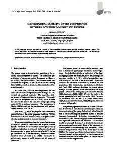
FIG. 3. Effect of diffusion on the infected population in a 10 ⫻10 lattice. We consider four values of the diffusion probability D ⬘ 共see text for details兲: 0 共dotted line兲, 0.1 共dashed line兲, 0.5 共dashdotted line兲, 1 共thin line兲. The AK model is depicted by the thick line. Rates b and c, in units of 1/⌬t, equal 0.5 and 0.2, respectively, the dimensionless quantity aK CS is 1.32, and the value of K CS in appropriate units is 66.
eral systems, with different values of the diffusion constant D, correspondingly of the dimensionless quantity D ⬘ ⫽D⌬t/(⌬x) 2 defined in Sec. I. It can be seen that the effect of diffusion on the bifurcation diagram is to lower the value of the critical carrying capacity. In fact, if the total probability for diffusion exceeds or equals 0.5, the infected population is almost indistinguishable from the one predicted by the mean field AK model. A small amount of transport between sites restores the unstable character of the state M I* ⫽0, providing for the necessary finite perturbation to take the system out of the trapped state.
IV. DISCUSSION
The deterministic model of Abramson and Kenkre has been found to be valid for diffusive situations with D ⬘ ⭓0.5 and for K values not too large (K⬍400). A critical behavior is also found in the probability evolution in the present simulations. For D ⬘ ⭓0.5, where mice transport destabilizes the M I* ⫽0 state, the critical value of the carrying capacity is as the one expected from the deterministic model. Nevertheless, for K⬎400, the simulations give equilibrium behavior 共for both types of mice populations兲 different from that predicted by the deterministic AK model. This difference can be observed in Fig. 4. The AK model predicts an underestimated and constant equilibrium value 共dashed line兲 for susceptible mice population and predicts an overestimated and linear increase for the infected population 共solid line兲. This should be compared to simulation data for M * S 共empty squares兲 and M I* 共filled squares兲. Both variations in the simulation lead to a total mice population that is in good accordance to the deterministic AK model. This behavior for high values of K may be understood if we can consider only two-mice interactions for the nonlinear
FIG. 4. Equilibrium values for total mice population AK model 共dotted line兲, simulation with diffusion 共filled dots兲; equilibrium values for susceptible mice population AK model 共dashed line兲, simulation with diffusion 共empty squares兲; equilibrium values for infected mice population AK model 共solid line兲, simulation with diffusion 共filled squares兲. Parameters values as in Fig. 1 and a value of D ⬘ ⫽1.
processes. If ⌬t/K(⌬x) 2 is the probability that a mouse at site ␣ dies as a result of competitive interaction with each of the other N ␣ mice present at the site ␣ , the probability ␣ ⫽1⫺„1 of dying from competition is p comp ␣ 2 (N ␣ ⫺1) ⫺⌬t/ 关 K(⌬x) 兴 … . Similar considerations apply to p inf . We have carried out simulations on the basis of these non␣ ␣ and p inf . They have shown, at least qualitatively, linear p comp the same results as those with their linear counterparts. While the nonlinear probabilities produce essentially the same results as linear ones, viz., a bifurcation to a state of positive infection at a finite value of K, the precise functional dependence of the bifurcation diagram as a function of K is different. We believe that only analysis of field data will be able to settle this matter in the two cases. An important observation is that the transition of a system with little diffusion to its equilibrium state takes longer if K is near the critical value. Thus, in a real landscape situation, equilibrium may never be reached by the mice population due to changes in the environment 共seasons, weather, etc.兲. Simulations have led us to a better understanding of the role of discreteness in mice number (⌬N⫽0) and fluctuation of finite number of mice (N⫽⬁). Both these factors tend, generally, to cause differences between simulations and moment equations. Further ongoing work along these lines includes the investigation of waves via simulation to make contact with recent work based on the AK model 关8兴 and a more microscopic study of the mice interactions by placing one rather than several mice at each site. These will be reported on elsewhere.
ACKNOWLEDGMENTS
The work presented in this paper was supported in part by a contract from Los Alamos National Laboratory to the
041908-4
SIMULATIONS IN THE MATHEMATICAL MODELING OF . . .
PHYSICAL REVIEW E 66, 041908 共2002兲
University of New Mexico, a grant from the National Science Foundation’s Division of Material Research 共Grant No. DMR0097204兲, and SECyT-University of Buenos Aires, Argentina 共Grant No. I046兲. Work at Los Alamos was sup-
ported by the U.S. Department of Energy. M. A. A. and G. A. acknowledge the support of the Consortium of the Americas for Interdisciplinary Science and the hospitality of the University of New Mexico.
关1兴 G. Abramson and V.M. Kenkre, Phys. Rev. E 66, 011912 共2002兲. 关2兴 G. Abramson and V. M. Kenkre, in Proceeding of Unified Science and Technology for Reducing Biological Threats and Countering Terrorism Conference 共BTR 2002兲, p. 64. 关3兴 J.N. Mills, T.L. Yates, T.G. Ksiazek, C.J. Peters, and J.E. Childs, Emerg. Infect. Dis. 5, 95 共1999兲. 关4兴 J.N. Mills, T.G. Ksiazek, C.J. Peters, and J.E. Childs, Proc. K. Ned. Akad. Wet., Ser. B: Palaeontol., Geol., Phys., Chem., Anthropol. 5, 135 共1999兲. 关5兴 M. Dresden, Rev. Mod. Phys. 33, 265 共1961兲.
关6兴 V.M. Kenkre, Z. Phys. B: Condens. Matter 43, 22 共1981兲. 关7兴 V.M. Kenkre and H.M. Van Horn, Phys. Rev. A 23, 3200 共1981兲. 关8兴 G. Abramson, V. M. Kenkre, T. L. Yates, and R. R. Parmenter, URL: http://arxiv.org/pdf/physics/0203088共physics/0203088兲 关9兴 E.J. Dawnkaski, D. Srivastava, and B.J. Garrison, J. Chem. Phys. 102, 9401 共1995兲. 关10兴 The factor 1/N(t) occurs because each mouse provides a clock, but all N clocks are running in parallel as explained, e.g., in P.L. Cao, Phys. Rev. Lett. 73, 2595 共1994兲.
041908-5