Simultaneous remote extraction of multiple speech sources and heart beats from secondary speckles pattern Zeev Zalevsky1*, Yevgeny Beiderman1, Israel Margalit1, Shimshon Gingold1, Mina Teicher2, Vicente Mico3 and Javier Garcia3 1
School of Engineering, Bar-Ilan University, Ramat-Gan 52900, Israel Dept. of Mathematics, Bar-Ilan University, Ramat-Gan 52900, Israel 3 Departamento de Óptica, Universitat de València, c/Dr. Moliner, 50, 46100 Burjassot, Spain * Corresponding author:
[email protected] 2
Abstract: The ability of dynamic extraction of remote sounds is very appealing. In this manuscript we propose an optical approach allowing the extraction and the separation of remote sound sources. The approach is very modular and it does not apply any constraints regarding the relative position of the sound sources and the detection device. The optical setup doing the detection is very simple and versatile. The principle is to observe the movement of the secondary speckle patterns that are generated on top of the target when it is illuminated by a spot of laser beam. Proper adaption of the imaging optics allows following the temporal trajectories of those speckles and extracting the sound signals out of the processed trajectory. Various sound sources are imaged in different spatial pixels and thus blind source separation becomes a very simple task. 2009 Optical Society of America OCIS codes: (070.0070) Fourier optics and signal processing; (280.1350) Backscattering
References and links 1.
Peter Yapp, "Who’s Bugging You? How Are You Protecting Your Information?," Information Security Technical Report 5, 23-33 (2000). 2. L. Hasan, N. Yu and J. Paradiso, "The Termenova: A hybrid free-gesture interface," Proceeding of the 2002 conference on new instrumentations for musical expression (NIME-02), Dublin, Ireland, May 24-26 2002. 3. SPIE session on biomedical OptoAcoustics, Vol. 3916, California (Jan. 2000): http://www.spie.org/web/meetings/programs/pw00/confs/3916.html 4. Z. Zalevsky and J. Garcia, "Motion detection system and method," Israeli Patent Application No. 184868 (July 2007). 5. J. C. Dainty, Laser Speckle and Related Phenomena, 2nd ed. (Springer-Verlag, Berlin, 1989). 6. H. M. Pedersen, “Intensity correlation metrology: a comparative study,” Opt. Acta 29, 105-118 (1982). 7. J. A. Leedertz, “Interferometric displacement measurements on scattering surfaces utilizing speckle effects,” J. Phy. E. Sci. Instrum. 3, 214-218 (1970). 8. P. K. Rastogi, and P. Jacquot, “Measurement on difference deformation using speckle interferometry,” Opt. Lett. 12, 596-598 (1987). 9. T. C. Chu, W. F. Ranson and M. A. Sutton, "Applications of digital-image-correlation techniques to experimental mechanics," Exp. Mech 25, 232-244 (1985). 10. W. H. Peters and W. F. Ranson, “Digital imaging techniques in experimental stress analysis,” Opt. Eng. 21, 427–431 (1982). 11. N. Takai, T. Iwai, T. Ushizaka, and T. Asakura, “Zero crossing study on dynamic properties of speckles,” J. Opt. (Paris) 11, 93–101 (1980); 12. K. Uno, J. Uozumi, and T. Asakura, "Correlation properties of speckles produced by diffractal-illuminated diffusers," Opt. Commun. 124, 16-22 (1996).
#109714 - $15.00 USD
(C) 2009 OSA
Received 6 Apr 2009; revised 16 Jun 2009; accepted 16 Jun 2009; published 11 Nov 2009
23 November 2009 / Vol. 17, No. 24 / OPTICS EXPRESS 21566
13. J. García, Z. Zalevsky, P. García-Martínez, C. Ferreira, M. Teicher, Y. Beiderman and A. Shpunt, "3D Mapping and Range Measurement by Means of Projected Speckle Patterns," Appl. Opt. 47, 3032-3040 (2008). 14. J. Garcia, Z. Zalevsky and D. Fixler, "Synthetic aperture superresolution by speckle pattern projection," Opt. Express 13, 6073-6078 (2005). 15. D. Bansal, B. Raj and P. Smaragdis, "Bandwidth expansion of narrowband speech using non negative matrix factorization," paper TR2005-135, 9th European Conference on Speech Communication (Eurospeech) 2005. 16. High speed digital cameras: http://www.photron.com/
1. Introduction Usage of optical means for detection of sounds has been used before mainly for security and trapping related applications where laser beam was projected on a window of a room in which interesting conversation was taking place. The light reflected from the window was collected and detected using optical interferometer and the sounds were extracted [1-3]. The idea was very simple: the speech sounds vibrate the window and those small vibrations are sufficient to perform detectable phase modulation in range of the optical wavelength. This configuration suffers from 4 major disadvantages. First, all sounds are detected together and in order to separate them one needs to apply digital blind source separation post processing algorithmic. Second, the projection laser and the detection interferometer module must be placed in very specific positions such that indeed the reflected beam should be directed towards the detection module. Third, the detection module is complicated and sensitive to errors as all interferometer based configurations. Fourth, it requires a window to be positioned near the voice source. In this paper we propose a new patented approach [4] overcoming all the four disadvantages that we have described. Our configuration includes projection of laser beam and observation of the movement of the secondary speckle pattern that are created on top of the target. The speckles are self interference random patterns [5] and have the remarkable quality that each individual speckle serves as a reference point from which one may track the changes in the phase of the light that is being scattered from the surface [5]. Because of that, speckle techniques such as electronic speckle-pattern interferometry (ESPI) have been widely used for displacement measuring and vibration analysis (amplitudes, slopes and modes of vibration) as well as characterization of deformations [6-12]. In case of an object deformations measurement, one subtracts the speckle pattern before the deformation has occurred (due to change in loading, change in temperature, etc.) from the pattern after loading has occurred. This procedure produces correlation fringes that correspond to the object’s local surface displacements between the two exposures. From the fringe pattern both the magnitude and the direction of the object’s local surface displacement is determined [7, 8]. Usage of speckles was also applied for improving the resolving capabilities of imaging sensors [13] as well as ranging and 3D estimation [14]. In our configuration the detection is obtained via fast imaging camera that observes the temporal intensity fluctuations of the imaged speckles pattern and their trajectory. In order to allow correlating the trajectory with the movement of the speckle patterns we had to properly defocus our imaging lens. Since the speckles are spatially small spots their diffraction occurs in wide angle (close to 2π Ste-Radians) and thus no matter where the camera is placed the speckles pattern may be imaged. Therefore no constrain exists any more regarding the location of the detector or the reflecting object. The speckles are self interfering pattern and thus the detection is done only by simple imaging so the detection module is not an interferometer and thus it is less sensitive to noises. Since the detection is realized with an imaging module, the temporal variations of any pixel in the image can be associated with different sound source and therefore one may realize
#109714 - $15.00 USD
(C) 2009 OSA
Received 6 Apr 2009; revised 16 Jun 2009; accepted 16 Jun 2009; published 11 Nov 2009
23 November 2009 / Vol. 17, No. 24 / OPTICS EXPRESS 21567
blind source separation of sounds just due to the spatial separation without the need for digital post processing. The bandwidth of speech signals is approximately 4KHz [15] and thus sampling at rate of 8Kfps is enough for the reconstruction. Nowadays digital cameras can allow even higher sampling frame rate at predefined spatial regions of interest of e.g. 256 by 256 pixels (this region for instance can potentially separate 256x256 different sound sources) [16]. The proposed approach was experimentally proven not only to detect acoustic and speech signals but also was capable of tapping cellular phones as well as detecting the heart beats temporal signature (resembles the ECG signals in medicine) of subjects positioned in noisy environmental scenario. Section 2 presents the theoretical explanation. Experimental results for voice detection, cellular phones taping and remote heart beats signature extraction are presented in section 3. The paper is concluded in section 4. 2. Theoretical explanation Speckles are self interfered random patterns. Speckle pattern can be generated by illuminating an object through a diffuser or a ground glass. Speckle patterns are generated due to the roughness of the surface of the object when illuminated by a spot of laser beam. When spatially coherent beam is reflected from the object whose roughness generates random phase distribution, in the far field we may obtain the self interfering speckle pattern. In the proposed configuration we propose not to focus the camera on the object but rather to have the camera focused on the far or close field such that the object itself is defocused. Doing that makes the movement of the object (its vibrations) to cause to a lateral shift of the speckles pattern. Actually due to this defocusing, the movement of the object instead of constantly changing the speckle pattern creates a situation in which we see the same speckle pattern which is only moving or vibrating in the transversal plane. This is very important feature since it allows, by tracking the maxima intensity spots, the extraction of the trajectory movement. As to be shown in the experimental part, the speech signals are vibrations around the trajectory of the entire object. The suggested approach allows not only extraction of the temporal speech and heart beat information but also estimating the 3D trajectory of the object. Let us now prove that indeed when slightly defocusing, instead of changing, the speckles pattern is moving. We will refer to Fig. 1 in order to explain our considerations. We will denote by (x,y) the coordinates of the transversal plane while the axial axis will be denoted by Z. Laser spot with diameter of D is illuminating normally a diffusive object. λ is the optical wavelength. The reflected light is imaged by a lens onto a detector giving a speckle pattern. This random amplitude and phase pattern is generated due to the random phase of the surface of the diffusive object. In the regular case the imaging system is imaging the plane close to the object determined by distance Z1 and in this case the amplitude distribution of the speckles equals to the Fresnel integral performed over the random phase φ that is created by the surface roughness. πi Tm ( xo , yo ) = ∫∫ exp [iφ ( x, y )] exp ( ( x − xo )2 + ( y − yo )2 ) dxdy = Am ( xo , yo ) exp [iψ ( xo , yo )] Z λ 1 (1) where paraxial approximation has been assumed, as well as uniform reflectivity over the object’s illuminated area. This distribution is viewed by the imaging device and the intensity of the obtained image equals to:
I ( xs , ys ) =
∫∫ T
m
( xo , yo )h( xo − Mxs , yo − Mys )
2
(2)
where h is the spatial impulse response and M is the inverse of the magnification of the imaging system. h takes into account the blurring due to the optics as well as due to the size of the pixels in the sensor and it is computed in the sensor plane (xs,ys). #109714 - $15.00 USD
(C) 2009 OSA
Received 6 Apr 2009; revised 16 Jun 2009; accepted 16 Jun 2009; published 11 Nov 2009
23 November 2009 / Vol. 17, No. 24 / OPTICS EXPRESS 21568
M=
( Z 2 + Z 3 − Z1 ) − F F
(3)
F is the focal length of the imaging lens. In the case of remote inspection, typically the distance object-lens is much longer that any other distance involved in the process. Assuming a rigid body movement, the movement of the object can be classified into three types of movements which can not be separated and they occur simultaneously: transverse, axial and tilt. Under transversal movement the amplitude distribution of the speckles pattern Tm will simply shift in x and in y by the same distance as the movement of the object, as can be checked in Eq. 1. Under normal imaging conditions and small vibrations, this movement will be demagnified by the imaging systems resulting in barely detectable shifts on the image plane. The second type of movement is axial movement in which the speckles pattern will remain basically the same since the variations in Z1 (which will only scale the resulted distribution) are significantly smaller in comparison to the magnification of the camera: Z + Z 3 Z 2 − Z1 + Z 3 (4) M= 2 ≈ F
F
The third type of movement is the tilt of the object which may be expressed as follows: πi Am ( xo , yo ) = ∫∫ exp [iφ ( x, y )] exp i ( β x x + β y y ) exp ( ( x − xo )2 + ( y − yo )2 ) dxdy λ Z 1
βx = βy =
4π tan α x
λ 4π tan α y
λ
(5) The angles αx and αy are the tilt in the x and y axes respectively and the factor of 2 accounts for the back and forth axial distance change. In this case and it is well seen from the last Eq., the resulting speckle pattern will change completely. Especially after the blurring of the small speckles with the impulse response of the imaging system having the large magnification factor (M can be a few hundreds) as described by Eq. 2. Since the three types of movements can not be separated, basically the speckles pattern is varied randomly. It should be noted that for small Z1 values the size of the speckles pattern at the Z1 plane will be very small and will not be visible in the sensor after imaging with large demagnification. Under these conditions the speckles associated with the aperture of the lens (the blurring width of λF# which is properly magnified when transferred to Z1 plane) is dominant (rather than the under-sampling due to the detector). Assuming now that we strongly defocus the image captured by the camera. Defocusing brings the plane of the imaging from position at distance of Z1 into a plane positioned at distance of Z2. In this case several changes occur. First, the magnification factor M is relatively small (it is reduced at least by one order of magnitude). Second, the plane at which the speckles pattern that are imaged by the camera is formed is in the far field approximation regime (the relevant speckle plane is far from the object). Therefore, the equivalent of Eqs. 1 and 2, is: −2π i Tm ( xo , yo ) = ∫∫ exp [iφ ( x, y ) ] exp ( xxo + yyo ) dxdy = Am ( xo , yo ) exp [iψ ( xo , yo )] (6) λ Z 2 and
I ( xs , ys ) =
∫∫ Tm ( xo , yo )h( xo − Mxs , yo − Mys )
2
(7)
Note that now also: M=
#109714 - $15.00 USD
(C) 2009 OSA
Z3 − F Z3 ≈ F F
(8)
Received 6 Apr 2009; revised 16 Jun 2009; accepted 16 Jun 2009; published 11 Nov 2009
23 November 2009 / Vol. 17, No. 24 / OPTICS EXPRESS 21569
Therefore in the case of transversal movement the speckles pattern is almost unchanged since shift does not affect the amplitude of the Fourier transform and because the magnification of the blurred function h is much smaller. Axial movement does not affect the distribution at all as well since Z2 is much larger than the shifts of the movement (only a constant phase is added in Eq. 6). Tilting is expressed as shifts of the speckles pattern. It is clearly seen in Fig. 1 as well as understood from Eq. 9 (linear phase is shift in the far field): −2π i Am ( xo , yo ) = ∫∫ exp [iφ ( x, y )] exp i ( β x x + β y y ) exp ( xxo + yyo ) dxdy λ Z 2
βx = βy =
4π tan α x
(9)
λ 4π tan α y
λ
The three types of movement are not separated but since now two of them produce negligible variations in the imaged speckle pattern, the overall effect of the three of them is the only the pure shift which may easily be detected by spatial pattern correlation. The resolution or the size of the speckle patterns that is obtained at Z2 plane and imaged to the sensor plane equals to: λ Z 1 λ F Z2 (10) δx= 2 ⋅ = ⋅ D M D Z3 This is of course assuming that this size of δx is larger (and therefore is not limited by) than the optical as well as the geometrical resolution of the imaging system. The conversion of angle to the displacement of the pattern on the camera is as follows:
d=
Z 2α Z 2 F = M Z3
(11)
Tilting angle
α Speckle patterns Diffusive object
Imaging module Sensor
α D
Laser projection Z1 Z2
Z3
Fig. 1. Schematic description of the system.
Note that assuming that ∆x is the size of the pixel in the detector then the requirement for the focal length is (we assume that every speckle in this plane will be seen at least by K pixels):
F=
K ∆x Z3 D Z 2λ
(12)
Note that Z2 fulfills the far field approximation: #109714 - $15.00 USD
(C) 2009 OSA
Received 6 Apr 2009; revised 16 Jun 2009; accepted 16 Jun 2009; published 11 Nov 2009
23 November 2009 / Vol. 17, No. 24 / OPTICS EXPRESS 21570
Z2 >
D2 4λ
(13)
The number of speckles in every dimension of the spot equals to:
N=
φ Mδ x
=
φD F ⋅D = λ Z 2 F# λ Z 2
(14)
where φ is the diameter of the aperture of the lens. F# is the F number of the lens. Mδx is the speckle size obtained at plane of Z2. This relation is obtained since the spot of the lens is covered by the light coming from the reflecting surface of the object. Eqs. 12 and 14 determine the requirements for the focal length of the imaging system. There contradictory requirements on both Eqs. On one hand, from Eq. 12 it is better to have small F since then the speckles are large in the Z2 plane (especially for large Z2) and it is preferred to increase the demagnification factor such that it will be easier to see the speckles with the pixels of the detector. In Eq. 14 we prefer larger F in order to have more speckles per spot. Therefore, a point of optimum may be found. This point limits the sound detection performance to few hundreds of meters. Let us make a small computation: Assuming D=1cm, Z2=100m, Z3=1m, N=3, F#=1.5, λ=0.8µm and ∆x=6µm one obtains: F=36mm, K=48. It is clear that K can not be too large since K·N is the region of interest and since we sample at high rate, this window should be as small as possible. Usually when sampling at rates of 8KHz or so (for recovering speech signals) the window should not exceed about 100 pixels in every direction and therefore the range of Z2=100 is close to the theoretical limit of detection. 3. Experimental results
3.1 Preliminary characterization In the first experiment we tried to extract the sounds of macroscopically static objects as loudspeakers. The object was illuminated by a doubled Nd:YAG laser with output power of 30mW at wavelength of 532nm. A conventional TVlens 16 mm focal length and F number of around 5.6 to 8 was used to image the speckle pattern. The camera was a Basler A312f with 8.3µm x 8.3µm pixels. The camera was controlled with Matlab. The camera can give up to 400 frames per second on small window of interest. The objects were illuminated through an X10 lens (with pinhole) that was positioned side by side to the camera. The object was positioned at approximately 1m away from both the camera and the laser source. In the left loudspeaker we have sent signals with increasing temporal frequency while to the right loudspeaker it was descending. Figure 2(a) presents an image of the loudspeakers as seen by the camera. The 10 by 10 pixels samples were taken from the spatial region which is the plastic of the loudspeakers (not the membrane itself). There are samples for both left and right loudspeakers. We captured 5000 frames in 12.207 seconds, giving 409.6 fps (Nyquist frequency of 205 Hz). The samples are analyzed with the Matlab function “specgram” that uses a default window of 256 pixels. The spectrogram is a time frequency representation which in this case has the size of 129x38 pixels (freq x time). In Fig. 2(b) we present the time sequence captured by the left loudspeaker. For clarity the upper right part of the image is a zoom of this temporal sequence. In Fig. 2(c) we present the spectrogram reconstructed from the left loudspeaker. It matches perfectly to the signals that were sent to it. The image processing we applied was a basically a correlation identifying the average shift of the speckles pattern. The variation of the position of the correlation peak is the extracted temporal acoustic signal. In Fig. 2(d) we present the spectrogram information reconstructed from the right loudspeaker. The reconstruction was obtained by applying similar digital processing. Here as
#109714 - $15.00 USD
(C) 2009 OSA
Received 6 Apr 2009; revised 16 Jun 2009; accepted 16 Jun 2009; published 11 Nov 2009
23 November 2009 / Vol. 17, No. 24 / OPTICS EXPRESS 21571
well a perfect match exists between the signals sent to the loudspeakers and the reconstruction.
(a).
(b).
(c).
(d).
Fig. 2. (a). The image of the loudspeakers. (b). The signal sent to the left loudspeakers. (c). The reconstructed spectrogram of the left loudspeaker. (d). The reconstructed spectrogram of the right loudspeaker.
In the next experiment we tried to extract speech signals directly by illuminating people. We have illuminated the throat as test point. We used the same Basler 312f camera with maximal resolution of 782x582 and used a region of interest of 20x20 and 20x40 pixels (The camera speed is almost independent of the width of the region of interest). The shutter was in the 40 to 100 microseconds range, and we used a Computar telecentric lens with focal length of 55mm. The aperture was 2.8. The illuminating laser was a Suwtech double Nd-YAG at power of approximately 1-20 mW. Figures 3(a) and 3(b) shows the speckle patterns. In two subsequent frames. Figure 3(c) presents the defocused image of the target person where the laser spot illuminates his/her throat. The images were correlated for shift finding. The result of the reconstructed temporal signal is presented in Fig. 3(d). Its spectrogram is seen in Fig. 3(e). The acoustic signal was a scream and indeed it was reconstructed in the proposed approach. The scream is marked in the spectrogram with an arrow. 3.2 Full outdoors testing In this subsection we present measurements in which we were able to detect direct speech signals in noise environment of standing and walking subjects, to hear their breathing and hear beats and to tape a cellular phone conversation.
#109714 - $15.00 USD
(C) 2009 OSA
Received 6 Apr 2009; revised 16 Jun 2009; accepted 16 Jun 2009; published 11 Nov 2009
23 November 2009 / Vol. 17, No. 24 / OPTICS EXPRESS 21572
(a).
(c).
(b).
(d).
(e).
Fig. 3. (a).-(b). Two consequential speckle patterns. (c). The defocused image of the target with the projected spot on top of it. (d). The extraction of the temporal speech signal (a scream). (e). The spectrogram of the signal of 3d.
In Fig. 4 we present one of the setups we tested. This configuration is capable of detecting voice signals at distances of few tens of meters. It used CANNON 28mm-300mm lens (F3.56.3). For larger distances we used a telescope instead of the CANNON lens. The camera model is PixelLink model number of A741. This camera can reach 7800 fps in reduced region of interest. In most experiments we worked with a region of interest of about 64 x 64 pixels at operation rates of about 2480 fps. Note that all the presented experiments, except for the last one, were performed with green laser (doubled Nd:YAG) that illuminated the subject in order to extract the speech signals. The last experiment was done with infrared laser at 915nm. All results were obtained by applying basic detection algorithm without any real post processing for noise removal. Therefore much better results can be extracted after proper post processing. All recordings with the visible laser were performed outside at noon and in the summer with strong turbulence effects and in an extremely noise environment between the recording system and the target.
Camera
Imaging lens Laser
Fig. 4. One of the experimental setups for far range detection.
#109714 - $15.00 USD
(C) 2009 OSA
Received 6 Apr 2009; revised 16 Jun 2009; accepted 16 Jun 2009; published 11 Nov 2009
23 November 2009 / Vol. 17, No. 24 / OPTICS EXPRESS 21573
The processing included correlation of the defocused speckles patterns and tracking the change in the position of the peak. This change in the position is the acoustic signal we aim to extract. In Fig. 5 we tape to a cellular phone conversation. The range is 60 meters and the sampling was performed at 2480 fps. The recording is of counting in English of 1,2,3,4,5,6. In Fig. 5(a) we present the image captured with our imaging system while in Fig. 5(b) one may hear the reconstructed taped signal.
(.wav) (a). (b). Fig. 5. Taping cellular phone. The person on the other side of the line is counting 1,2,3,4,5,6... (a). Image of the cellular phone. (b). (Media 1) The reconstructed taped signal.
In Fig. 6 we demonstrate the reconstruction of speech signal from the back part of the head without seeing the face of the speaker. The range was about 30 meters. The recording was at 2480 fps. The subject is saying in English: 5,6,7. In Fig. 6(a) we present the scenario while in Fig. 6(b) we show the reconstructed signal.
(.wav) (a). (b). Fig. 6. Listening to talks from the back part of the neck. The person is counting 5,6,7... (a). Image of the subject. (b). (Media 2) The reconstructed signal.
Next we performed a recording at range of 100 meters by observing the speckles pattern reflected from the face. The recording was performed across noisy constriction site. The sampling was at 2480 fps. The voice file contains counting in English saying 5,6... Figure 7(a) presents the scenario while in Fig. 7(b) we show the reconstructed voice signal. In the next experiment we aimed to extract the heart beating signature rather than the speech signals. We illuminated the side of the neck from 60 meters. The sampling rate was 2480 fps. In Fig. 8(a) we present the scenario while in Fig. 8(b) we show the reconstructed heart beats signal.
#109714 - $15.00 USD
(C) 2009 OSA
Received 6 Apr 2009; revised 16 Jun 2009; accepted 16 Jun 2009; published 11 Nov 2009
23 November 2009 / Vol. 17, No. 24 / OPTICS EXPRESS 21574
(.wav) (a). (b). Fig. 7. Listening to talks from the profile of the face. The person is counting 5,6…. (a). Image of the subject. (b). (Media 3) The reconstructed signal.
As a clarifying example, in Fig. 9(a) we present the reconstruction of speech signal containing a counting in English (obtained in the previous experiments) and in Fig. 9(b) we show its spectrogram.
(.wav) (a). (b). Fig. 8. Listening to heart beats. (a). Image of the subject. (b). (Media 4) The reconstructed signal.
The units of the temporal axis in Fig. 9(a) are 1/2480 sec (each 2480 pixels are 1 sec). The horizontal units in Fig. 9(b) are in seconds. The vertical units are in Hz. One may clearly see both in the temporal signal as well as in the spectrogram how the words are well separated in time and well visible. Signal Reconstruction
Spectrogram
2
0
1.5
200 1
400 0.5
600
0 -0.5
800 -1
1000 -1.5 -2
(a).
(b). 1200
0
1000
2000
3000
4000
5000
6000
7000
8000
9000 10000
0
0.5
1
1.5
2
2.5
3
3.5
Fig. 9. (a). The temporal voice signal. (b). The spectrogram.
#109714 - $15.00 USD
(C) 2009 OSA
Received 6 Apr 2009; revised 16 Jun 2009; accepted 16 Jun 2009; published 11 Nov 2009
23 November 2009 / Vol. 17, No. 24 / OPTICS EXPRESS 21575
The temporal signal and the spectrogram of the heart beats signals is seen in Fig. 10(a) and 10(b) respectively. Once again the beats are very visible. The units in Fig. 10(a) are in 2.5/10 [sec]. The horizontal units in Fig. 10(b) are in seconds and the vertical are Hz. Signal Recognition 1
1200
0.8 1000
0.6 0.4
800 Frequency
0.2 0 -0.2
600
400
-0.4 -0.6
200
(a).
-0.8 -1
(b). 0
0
0.5
1
1.5
2
1
2.5
2
3
4
4
5 Time
6
7
8
9
Fig. 10. Experimental results for heart beats detection of remote subject. (a). The temporal signal. (b). The spectrogram.
Now we performed recording through a glass window. The range was about 30 meters. The recording was at 2480 fps. The recording is from the forehead. Signal Reconstruction
Spectrogram
1.5
0
1
200
0.5
400
600
0
800
-0.5
1000
-1
(a). -1.5
0
10000
15000
(c).
(b).
1200
5000
0
1
2
3
4
5
Fig. 11. Experimental results for recording through a window at 30 meters across very noise construction site of talking subject. Recording from forehead. (a). The temporal signal. (b). The spectrogram. (c). The scenario of the experiment.
In Fig. 11 we present experimental results for recording through a window at 30 meters across very noise construction site of talking subject. The recording is done from the forehead. 1.5 1.5
0
11
200
0.5 0.5
400 600
00
800
-0.5 -0.5
1000
- 1-1 -1.5 -1.5
(a).
(b). 1200
0
0
1000
1
2000
2
3000
3
4000
4
5000
5
6000
6
7000
7
8000
8
9000
9
10000 10
0
0.5
1
1.5
2
2.5
3
3.5
Fig. 12. Experimental results for speech detection with IR laser. (a). The temporal signal. (b). The spectrogram.
#109714 - $15.00 USD
(C) 2009 OSA
Received 6 Apr 2009; revised 16 Jun 2009; accepted 16 Jun 2009; published 11 Nov 2009
23 November 2009 / Vol. 17, No. 24 / OPTICS EXPRESS 21576
In Fig. 11(a) we present the temporal signal each pixel is 1/2480 of a second. In Fig. 11(b) we present the spectrogram of the signal while the scenario of the experiment is seen in Fig. 11(c). The subject appearing in the left part of Fig. 11(c) is illuminated with a laser spot (marked with red arrow). The last experiment contained recording with infra red laser at 915nm (it is important due to eye safety issues). It was done in the laboratory at range of 3 meters. The recording was done from the forehead. Figure 12(a) presents the temporal signal and Fig. 12(b) is its spectrogram. One can clearly see the separate words of the counting in English in the temporal signal as well as in its spectrogram. Each temporal scale of one is equivalent to 1000/2480 of a second. (a).
(b).
X=287
X=279
0
50
100
150
200
250
300
350
400
450
500 0
(c).
150
200
250
300
350
(d).
X=506
X=509
400
450
500
550
600
(e).
400
450
500
550
600
(f). X=510 X=507
350
400
450
500
550
600
650
300 350
400
450
500
550
600
650
700
750
Fig. 13. Spectral components of OCG signature. (a)-(d) Reconstruction after projecting on hand joints. (e)-(f) Reconstruction after projection on the throat. (a). Subject #1 at rest sampled at 20Hz. (b). Subject #1 at physical strain while sampled at 20Hz. (c). Subject #2 at rest while sampled at 100Hz. (d). Subject #2 at physical strain while sampled at 100Hz. (e) Subject #3 at rest while sampled at 100Hz. (f). Subject #3 at physical strain while sampled at 100Hz.
#109714 - $15.00 USD
(C) 2009 OSA
Received 6 Apr 2009; revised 16 Jun 2009; accepted 16 Jun 2009; published 11 Nov 2009
23 November 2009 / Vol. 17, No. 24 / OPTICS EXPRESS 21577
3.3 Optical cardio-gram measurement As previously mentioned and demonstrated the system and the operation principle which we used for detecting tilted movement can also be used to extract not only speech signals but also optical signals corresponding to ECG. We will coin those signals as Optical Cardio-Gram (OCG). Those signals can indicate the pressure condition and the physical stress of an individual as well as to separate the temporal signature of a certain individual from another one. In this subsection, we measure those signals and show their dependency on different subjects and their physical condition as well test the repeatability of such measurements with time. We used the same digital camera: PixelLink model number of A741. We took spatial region of 128 by 128 pixels. The camera and the laser were positioned side by side. The distance between the camera and the subject was about 1m. The camera was focused at far range behind the subject. We used Nd:YAG laser with wavelength of 532nm. X - movement
CorrLine: pulses marked
45
25
(a).
40
(b).
Peak captured
20
35 15
30 25
10
20
5
15
0
10 -5
5 -10
0 -5
-15
0
100
200
300
400
500
600
700
800
900
1000
0
100
200
300
400
X - movement
(c).
650
700
750
800
850
900
700
800
900
1000
300
350
400
450
500
550
X - movement
(e).
140
600
(d).
X - movement
120
500 X - movement
(f).
160
180
200
220
240
260
280
300
320
550
600
650
700
750
800
Fig. 14. Temporal OCG signature. (a). Temporal signature of subject #4. (b). Temporal signature of subject #5 and correlation peaks designating that indeed its temporal signature is repeatable. (c). Temporal signature of subject #6. (d). Temporal signature of subject #6 recorded in a different day. The signature is repeatable. (e). Temporal signature of subject #7. (f). Temporal signature of subject #8. Different subjects have different signature.
#109714 - $15.00 USD
(C) 2009 OSA
Received 6 Apr 2009; revised 16 Jun 2009; accepted 16 Jun 2009; published 11 Nov 2009
23 November 2009 / Vol. 17, No. 24 / OPTICS EXPRESS 21578
Some results are presented in Fig. 13. In Fig. 13(a)-13(b) the laser beam was projected on the hand joints and performed measurements at 20Hz. We took 500 samples and therefore the spectral resolution should be 1/(500/20)=0.04Hz. Control measurement was performed with Polar Clock heart rate monitor and the result was 1.33pulses/sec. Since the Fourier was performed over a set of 490 pixels the expected position for the spectral peak is at pixel number 245+1.33/0.04=278. As one may see the peak was obtained at pixel 279 which corresponds with the external measurement by the Polar Clock. The same measurement was repeated for the same subject at physical strain. This time the external measurement was 1.783 (pulses per second). Therefore the anticipated peak should appear at pixel number 245+1.783/0.04=289. The peak was obtained at pixel 287, at only 0.7% from the external measurement. The measurements at Fig. 13(c)-13(f) were performed at rate of 100Hz. 1000 temporal images were taken (i.e. time window of 10 seconds). For Fig. 13(c) the Polar Clock measurement gave the result of 1.033 pulses per second. In this case the spectral resolution is 1/(1000/100)=0.1Hz and therefore since we took in the spectral computation only 990 pixels, the anticipated peak should appear at pixel number 1.033/0.1+495=505.3 while it was obtained at 506. In Fig. 13(d) the Polar Clock measurement gave 1.433 pulses per second and therefore we anticipate having peak at pixel number: 1.433/0.1+495=509.3. The peak was obtained at 509. In Fig. 13(e) the Polar Clock gave result of 1.216 and therefore the peak is anticipated at pixel 1.216/0.1+495=507.2. The peak was obtained at pixel number 507. In Fig. 13(f) the Polar Clock gave 1.5 pulses per second and therefore the peak is anticipated at pixel: 1.5/0.1+495=510 and indeed we have received it at pixel 510. (b).
(a).
P ers on Iden tific ation by P u ls e F rom an E xis tin g P ool (P erc entag e) 100%
13.3
Non-Identification Multi Identifications - More Than Four persons Identified
80%
13.3
60%
16.6
10
Up to Four Persons Identified 40% 46.6
Double Identifications 20% Perfect Identification
(c).
0%
P ers on Iden tific ation by P u ls e P erc en tag e of S u c c es s an d E rror 86.6 58.7 41.3 13.3
The Examinee Is Not The Examinee Is Not The Examinee Is Part The Examinee Is Part Part Of The Pool And Part Of The Pool But Of The Pool But Not Of The Pool And Not Identified Identified Identified Identified
Fig. 15. Using OCG for identifying individuals. (a). The measurement configuration. (b). Identification of subjects from an existing pool. (c). Percentages of success and error.
#109714 - $15.00 USD
(C) 2009 OSA
Received 6 Apr 2009; revised 16 Jun 2009; accepted 16 Jun 2009; published 11 Nov 2009
23 November 2009 / Vol. 17, No. 24 / OPTICS EXPRESS 21579
In Fig. 14 we tested the temporal signature of the OCG signals. In Fig. 14(a) one may see the temporal signature of a subject while the signature i.e. a single period is enlarged. The parameters of the experiment are identical to the one of Fig. 13 while the sampling was at 100Hz. In Fig. 14(b) one may see the temporal signature of different subject with correlation peaks appearing on top of it indicating the preservation of its unique temporal shape. In Fig. 14(c) and 14(d) we present the temporal signature of subject #6 at rest in different days. The signature is repeatable. In Figs. 14(e) and 14(f) we present the temporal signature of subjects #7 and #8. Different subjects have indeed different signatures. In short range OCG measurement stand that was constructed (depicted in Fig. 15(a)), we have tried to perform preliminary statistics on the capability to use the optically detected signature for identification of individuals. The measurements were done using Nd:YAG laser at 532nm which was installed and fixed as part of the measurement stand. The measurement was performed on a group of 30 subjects part of which were considered as a pool of signatures. Then, the OCG of the subjects was measured again and we have compared each one of the subjects to the signatures in the pool. In some cases the correlation was only for the subject with itself. Subjects in the pool were identified as such and those which are not were identified as such as well. In some cases measurement of a given subject in the pool that was identified resembled not only to his own signature but also to one, two or more different subjects in the pool. Sometimes subject that was not in the pool was identified as such etc. The statistics is summarized in the chart of Fig. 15(b) and 15(c). Although the algorithms that were applied for identification (simple correlation and thresholding) as well as the configuration were very preliminary we saw that more than 86% of the subjects we properly identified. Note that although all measurements in this work were performed using visible green laser at 532nm, a simple upgrade of the system can allow working with infra red light source which is also safe to the eyes. 4. Conclusions
In this paper we have presented a new approach for remote "hearing" via imaging. The proposed optical approach allows blind source separation of acoustic signals (e.g. speech signals). The main advantages of the suggested configuration are its simplicity and modularity, lack of restriction regarding the position of the system in comparison to the acoustic sources and the capability of separating several (even more than 2) sources without the need of applying sophisticated digital signal post processing algorithms. Experimental results presented the capabilities of the discussed approach for remote speech recording, extraction of heart beats temporal signature, cellular phone taping and hearing through wind
#109714 - $15.00 USD
(C) 2009 OSA
Received 6 Apr 2009; revised 16 Jun 2009; accepted 16 Jun 2009; published 11 Nov 2009
23 November 2009 / Vol. 17, No. 24 / OPTICS EXPRESS 21580