Size and Treewidth Bounds for Conjunctive Queries ∗
Georg Gottlob
Computing Laboratory and Oxford Man Institute of Quantitative Finance, University of Oxford,UK
Stephanie Tien Lee Computing Laboratory University of Oxford, UK
[email protected]
[email protected]
†
Gregory J. Valiant
Computer Science Division UC Berkeley Berkeley, CA, USA
[email protected]
ABSTRACT
Keywords
This paper provides new worst-case bounds for the size and treewith of the result Q(D) of a conjunctive query Q to a database D. We derive bounds for the result size |Q(D)| in terms of structural properties of Q, both in the absence and in the presence of keys and functional dependencies. These bounds are based on a novel “coloring” of the query variables that associates a coloring number C(Q) to each query Q. Using this coloring number, we derive tight bounds for the size of Q(D) in case (i) no functional dependencies or keys are specified, and (ii) simple (one-attribute) keys are given. These results generalize recent size-bounds for join queries obtained by Atserias, Grohe, and Marx (FOCS 2008). An extension of our coloring technique also gives a lower bound for |Q(D)| in the general setting of a query with arbitrary functional dependencies. Our new coloring scheme also allows us to precisely characterize (both in the absence of keys and with simple keys) the treewidth-preserving queries— the queries for which the output treewidth is bounded by a function of the input treewidth. Finally we characterize the queries that preserve the sparsity of the input in the general setting with arbitrary functional dependencies.
Database Theory, Conjunctive Queries, Size Bounds, Treewidth
Categories and Subject Descriptors H.2.4 [Database Management]: Systems—relational databases, query processing; F.2.0 [Analysis of Algorithms and Problem Complexity]: Miscellaneous
General Terms Algorithm Design, Theory ∗Georg Gottlob’s work was supported by EPSRC grant EP/E010865/1 “Schema Mappings and Automated Services for Data Integration and Exchange”. Gottlob also gratefully acknowledges a Royal Society Wolfson Research Merit Award. †Gregory Valiant’s work is supported under a National Science Foundation Graduate Research Fellowship.
Permission to make digital or hard copies of all or part of this work for personal or classroom use is granted without fee provided that copies are not made or distributed for profit or commercial advantage and that copies bear this notice and the full citation on the first page. To copy otherwise, to republish, to post on servers or to redistribute to lists, requires prior specific permission and/or a fee. PODS’09, June 29–July 2, 2009, Providence, Rhode Island, USA. Copyright 2009 ACM 978-1-60558-553-6 /09/06 ...$5.00.
1.
INTRODUCTION
In this paper we deal with the general question of how large and intricate the result of a conjunctive query can be, relative to the input relations. We derive worst-case size bounds for the result that depend only on structural properties of the query itself. We assess the intricacy of a data relation via measures of sparsity and treewidth. We derive bounds for the sparsity and treewidth of the result of a query and characterize those conjunctive queries that are sparsitypreserving as well as those that are treewidth-preserving. Conjunctive queries are the most fundamental and most widely used database queries [7, 20, 1] . They correspond to project-select-join queries in the relational algebra, and to SQL queries of the form SELECT . . . FROM . . . WHERE . . ., whose where-clause equates pairs of attributes of the relations mentioned in the from-clause. Conjunctive queries also correspond to nonrecursive datalog rules of the form R0 (u0 ) ← R1 (u1 ) ∧ . . . ∧ Rn (um ), where Ri is a relation name of the underlying database D, R0 is the output relation, and where each argument ui is a list of |ui | variables, where |ui | is the arity of the corresponding relation, and where the same variable can occur multiple times in one or more argument lists. We allow a single relation Ri to appear several times in the query, thus m ≥ n. Throughout this paper we adopt this datalog rule representation for conjunctive queries. It is obvious that, in general, the result of a conjunctive query can be exponentially large in the input size. Even in the case of bounded arities, the result can be substantially larger than the input relations. In fact, in the worst case, the output size is rk , where r is the size of the largest input relation and k is the arity of the output relation. Queries with very large outputs are sometimes unavoidable, but in most cases they are either ill-posed or anyway undesirable, as they can be disruptive to a multi-user DBMS. It is thus useful to recognize such queries, whenever possible. Obtaining good worst-case bounds for conjunctive queries is, moreover, relevant to view management [20] and data integration [19, 20], as well as to data exchange [11, 18], where data is transferred from a source database to a target database according to schema mappings that are specified via conjunctive queries. In this latter context, good bounds on the result size of a conjunctive query may be used for estimating the amount of data that needs to be materialized at the target site.
In the area of query optimization, models for predicting the size of the output of a conjunctive query based on selectivity indices for relational operators have been developed [24, 17, 8]. The selectivity indices are obtained via sampling techniques (see, e.g. [22, 16]) from existing database instances. Worst case bounds may be obtained by setting each selectivity index to 1, thus assuming the maximum selectivity for each operator. Unfortunately, the resulting bounds are then often trivial (akin to the above rk bound). A new and very interesting characterization of the worstcase output size of join queries was very recently developed by Atserias, Grohe, and Marx [5]. The join queries form a proper subclass of the conjunctive queries, and correspond to those conjunctive queries in which all query variables appear in the head atom R0 (u0 ). Their result is based on the notion of fractional edge cover [15], and the associated concept of fractional edge-cover number ρ∗ (Q) of a join query Q. In particular, in [15] it was shown that ∗
|Q(D)| ≤ rmax(Q, D)ρ
(Q)
,
(1)
where rmax(Q, D) represents the size of the largest relation among R1 , . . . , Rn in D. In [5] it was shown that this bound is essentially tight. A substantial part of the present paper deals with the question of whether it is possible to find similar tight worstcase bounds for the output of general conjunctive queries. In particular, we asked this question in three different settings: 1. for general conjunctive queries without integrity constraints; 2. for general conjunctive queries where simple keys have been specified on the underlying database D; and 3. for general conjunctive queries in the setting where arbitrary functional dependencies have been specified on D. We are able to derive tight bounds similar to those in Formula 1 for settings 1 and 2, and we can give a lower bound for the third (most general) setting. Moreover, for the third setting, we give a precise characterization of the sparsity preserving queries - those queries for which in each input database D with domain UD , the quotient |R0 |/|UD | for the output relation R0 is at most a constant factor larger than the quotient |D|/|UD |. A crucial step towards our results is the introduction of a new coloring scheme for query variables, and, accordingly, the association of a color number C(Q) with each query Q. Roughly, a valid coloring assigns a set L(X) of colors to each query variable X and requires that for each functional dependency V → W , the colors of W are contained in those of V . The color number C(Q) of Q is the maximum over all valid colorings of Q of the quotient of the number of colors appearing in the output (i.e., head) variables of Q by the maximum number of colors appearing in the variables of any input (i.e., body) atom of Q. By using the coloring number C(Q) instead of ρ∗ (Q), and by exploiting linear programming duality as in [5], we slightly generalize results of [5] by obtaining the following essentially tight worst-case bounds for the output size of general queries of the form R0 (u0 ) ← R1 (u1 ) ∧ . . . ∧ Rn (um ) without specified constraints (Setting 1): |Q(D)| ≤ rmax(Q, D)C(Q) ,
As a corollary we obtain a characterization of the sparsitypreserving queries: A query Q is sparsity-preserving iff C(Q) = 1. It turns out that the color number is equally useful in the case that simple keys are given on the underlying database (Setting 2). However, rather than coloring the original query Q, we color chase(Q), which is the result of chasing the keys over the query. The Chase [2, 21, 6, 10, 11] is a wellknown procedure for enforcing functional dependencies, and, in particular, keys. For example, let Q be r(X, Y, Z) ← s(X, Y )∧s(X, Z), where the first attribute of the relation s is a key for s, or equivalently, where the functional dependency s[1] → s[2] has been specified, then chase(Q) is the query r(X, Y, Y ) ← s(X, Y ). We prove the following essentially tight worst-case bounds for the case with simple keys: |Q(D)| ≤ rmax(Q, D)C(chase(Q)) . In case of simple keys (or even functional dependencies with single-attribute left sides) the color number C(chase(Q)) can be computed in polynomial time via a polynomial-time chase followed by the solution of a polynomially sized linear program. As a corollary, we show that when C(chase(Q)) is bounded, and when each query variable occurs in the output variables u0 , we immediately obtain a polynomial algorithm for query evaluation. For composite keys and arbitrary functional dependencies (Setting 3), we derive the same lower bound as for simple keys. While we currently do not know whether the upper bound rmax(Q, D)C(chase(Q)) carries over to this more general setting, we are able to characterize the sparsitypreserving queries. A query Q in this setting is sparsitypreserving iff C(chase(Q)) = 1. An important measure for describing the inherent intricacy of a graph or finite structure is treewidth [23]. The treewidth tw(D) of a structure D corresponds in a precise sense to its degree of cyclicity. For example, each tree has treewidth 1, each cycle has treewidth 2, the clique Kk of k elements has treewidth k − 1. By Courcelle’s theorem [9], all Boolean queries that can be expressed in terms of monadic second-order logic can be answered in linear time on structures (databases) of bounded treewidth. This result was actually generalized to a large class of queries based on monadic optimization problems [4]. By these results, interesting queries that cannot be formulated in SQL or first order logic, and that are NP-hard on arbitrary structures, can be answered in linear time on structures of bounded treewidth. Queries in this class include, for example, questions related to network multicuts [12], program flow graphs [25], or logic-based diagnosis [14]. One may not always issue such queries directly to the original database, but maybe to a view that has been defined via a conjunctive query. In this context, we posed ourselves the following questions: • Given a set of relations D of bounded treewidth and a conjunctive query Q. How large is the treewidth of Q(D)? • Is it possible to characterize the queries that preserve bounded treewidth in the sense that tw(Q(D)) = O(tw(D))? A join expression R 1A=B S is a keyed join if B is a key for S. We first observed that keyed joins are most beneficial
for treewidth preservation. (Here B may be a composite attribute.) We derived the following bound on the treewidth of the result of a keyed join R 1A=B S where R has arity k, and S has arity j, and tw(hR, Si) = ω and B is a key of S: tw(R 1A=B S) ≤ (j − 1)(ω + 1) − 1. Via a nontrivial example we show that this bound is tight up to a small constant factor. We also extend this bound to sequences of keyed joins and to conjunctive queries whose bodies consist of such sequences. For the case of (fixed) queries Q over (variable) input databases D without keys, we use colorings to precisely characterize the treewith-preserving queries: tw(Q(D)) = O(tw(D)) iff tw(Q(D)) ≤ tw(D) iff there exists no valid coloring of Q with two colors having color number two. We also consider the case where there are arbitrary keys that are not necessarily part of the join attribute. This case can be reduced to the previous case by chasing the keys. We characterize the queries which are treewidth-preserving in this setting, too. This paper is organized as follows. In Section 2 we state some useful definitions. In Section 3 we define the basic coloring scheme and the color number of a query. In later sections, we extended the basic coloring scheme to deal with keys, and ultimately, to general functional dependencies. Section 4 reports about our size-bounds both without keys and with simple keys, and also deals with sparsity-preservation for those cases. Section 5 presents all our results on treewidth. Section 6 deals with the extension of the work of Section 4 to the setting where arbitrary functional dependencies are specified on the underlying database. Some open problems and topics for future research are stated at the end of Section 6.
2.
PRELIMINARIES AND BASIC DEFINITIONS
We assume the reader to be familiar with the theory of relational database systems, relational algebra, and conjunctive queries. As already said in the Introduction, a conjunctive query has the form R(u0 ) ← R1 (u1 ) ∧ . . . ∧ Rn (um ), where each ui is a list of (not necessarily distinct) variables of length |ui | = arity(Ri ). Each variable occurring in the query head R0 (u0 ) must also occur in the body of the query. The set of all variables occurring in Q is denoted by var(Q). It is important to recall that a single relation Ri might appear several times in the query, and thus m could be larger than n. A finite structure or database D = (UD , R1 , . . . , Rk ) consists of a finite universe UD and relations R1 , . . . , Rk over UD . The answer Q(D) of query Q over database D consists of the structure (UD , R0 ) whose unique relation R0 contains precisely all tuples θ(u0 ) such that θ : var(Q) → UD is a substitution such that for each atom Ri (uj ) appearing in the query body, θ(uj ) ∈ Ri . For ease of notation, we define rmax(Q, D) to be the number of tuples in the largest relation among R1 , . . . , Rn in D. A (simple) attribute of a relation R identifies a column of R. An attribute list consists of a list (without repetition) of attributes of a relation R. A compound attribute is an attribute list with at least two attributes. A list consisting of a unique attribute A is identified with A. The list of
all attributes of R is denoted by attr(R). If V is a list of attributes of R and t ∈ R a tuple of R, then the V -value of t, denoted by t[V ] consists of the tuple obtained as the ordered list of all values in V -positions of t. If V and W are (possibly compound) attributes of R, then a functional dependency (FD) V → W on relation R expresses that for each t, t0 ∈ R, t[V ] = t0 [V ] implies that t[W ] = t0 [W ]. Thus each functional dependency V → W is equivalent to a set containing a FD V → A for each element A of W . If A and B are single attributes, then the FD A → B is called a simple FD. A (possibly compound) attribute K of R is a key iff K → attr(R) holds. Such a key is called a simple key if K is a simple attribute, otherwise it is called a compound key.1 An argument position in an atom that corresponds to a simple key attribute is referred to as a keyed position. Let D = (UD , R1 , . . . , Rk ) be a structure. The Gaifman graph G(D) of D is the graph (UD , E), where {a, b} ∈ E iff a and b are two distinct elements from UD who appear jointly in some tuple of D. Given a graph G = (V, E), a tree decomposition [23] of G is a pair (T, λ), where T = (N, A) is a tree, and λ a labeling function λ : N → 2V such that: (i) for all v ∈ V , there exists n ∈ N such that v ∈ λ(n); (ii) for all edges e ∈ E, there exists n ∈ N such that λ(n) ⊇ e; (iii) for every v ∈ V , the set {n ∈ N | v ∈ λ(n)} induces a connected subtree in T. The width of a tree decomposition (T, λ) is the integer value max{|λ(n)|−1 | n ∈ N }. The treewidth of a graph G = (V, E), denoted tw(G), is the minimum width of all tree decompositions. Given a finite structure D = (UD , R1 , . . . , Rk ), the treewidth of D is defined to be the treewidth of its Gaifman graph, formally tw(D) = tw(G(D)). The following motivating example shows that the size and treewidth of the result of a conjunctive query over a database D can be significantly larger than the size and treewidth of D, respectively. Example 2.1. Consider the relation R(A, B) = {h1, 1i, h1, 2i, . . . , h1, ni} that has treewidth 1. The relation R0 = R 1A=A R, which is equivalently obtained as the result of the conjunctive query R0 (X, Y, Z) ← R(X, Y ) ∧ R(X, Z), has n2 tuples where each of the n elements appears in a tuple with each of the other elements. Thus the Gaifman graph is the complete graph on n vertices, which has treewidth n − 1. Letting n get large, we see that the treewidth of R0 can be arbitrarily large, while the treewidth of R is still 1. Definition 2.2. For a database D, we define the sparsity of D to be sp(D) := |D|/|UD |, where |D| is the number of tuples in D, and |UD | is the number of elements in the domain of D. Remark If we are to consider the blowup of the sparsity after the application of a query Q, one could decide whether to define UQ(D) to be the same as UD , or whether we allow UQ(D) to be restricted to the active domain of Q(D), i.e., to those domain values that occur effectively in Q(D). In the 1
Note: We do not require compound keys to be minimal.
second case, even without increasing the number of tuples, by a single projection operation we can increase the sparsity (by, for example, removing all the key attributes). Even for a single keyed join, for any N , one can easily construct a relation R with sp(R) = 1 such that sp(R ./ R) = N . For this reason, in the remainder of this section our analysis will focus on the richer and more interesting problem of understanding the blowup in sparsity using the first definition, where we fix UQ(D) to be the same as UD . There is also a question of how to define the sparsity of a query input list hR1 , . . . , Rn i corresponding to a query body R1 (u1 ) ∧ . . . ∧ Rn (um ), given that this may contain repeated occurrences of the same relation Pm symbol. For convenience we define the sparsity to be j=1 |Ri(j) |/|UD |, that is, we double-countP relations that occur multiple times. If we were to only take n i=1 |Ri |/|UD | then one could concatenate all the Ri ’s to form a relation R with arity the sum of the arities of the Ri ’s, and |R| = maxi |Ri |, such that the result of applying the corresponding query with each Ri replaced by R is unchanged, but the sparsity would be smaller. Definition 2.3. A query Q over input relation list hR1 , . . . , Rn i (possibly with repeated relations) is sparsity preserving if for every database instance, sp(Q(hR1 , . . . , Rn i)) = O(sp(hR1 , . . . , Rn i)).
3.
THE COLORING
In this section we define a coloring scheme for assigning colors to the variables appearing in a conjunctive query. This coloring underlies both our tight bounds on the size of the results of the query, and our characterizations of queries that have bounded sparsity and bounded treewidth. We start by giving the basic definition that applies to the setting without any functional dependencies. In section 4.2 we extend this definition to accommodate simple keys, and finally in section 6 we further extend this definition in a natural way to the case where general functional dependencies are specified.
4.
SIZE BOUNDS AND SPARSITY
In this section we present our main results regarding size bounds and sparsity. We consider conjunctive queries without keys and with simple keys. Whenever we use the word “key” in this section we mean “simple key”. Essentially, the color number of a query will be a tight bound on the exponent relating the sizes of the input and the output database. We start this section by considering the special case in which the given query has no keyed relations, and relate our characterization to previous results regarding size bounds. We will then reduce the general case with keys to this special case.
4.1
Size Bounds Without Keys
We begin by considering the case when no relations have keys. While this case has been considered in [15, 5], our approach will allow us to extend the results to the case with specified output variables and keys. Proposition 4.1. Given a query Q = R0 (u0 ) ← R1 (u1 )∧ . . . ∧ Rn (um ) without specification of FDs or keys, for any database D, |Q(D)| ≤ rmax(Q, D)C(Q) , where rmax(Q, D) is the size of the largest relation among R1 , . . . , Rn in D. Furthermore, this bound is essentially tight: for any integer N > 0, there exists a database D with rmax(Q, D) ≤ rep(Q) · N , and |Q(D)| = N C(Q) , where rep(Q) is defined to be the maximum number of times any specific relation Ri appears in Q. Corollary 4.2. A query Q, as in Proposition 4.1, without FDs or keys is sparsity preserving if, and only if C(Q) = 1. Equivalently, Q is sparsity preserving if, and only if ∃i ≥ 1 such that the variables in u0 are a (not necessarily proper) subset of the variables of ui .
To prove Proposition 4.1 we first show that C(Q) is the solution to a linear program, then, exploiting duality, reduce it to the upper bound given in [15, 5]. Definition 3.1. Given a conjunctive query Q = R0 (u0 ) ← Proof of proposition 4.1: Given a query R0 (u0 ) ← R1 (u1 ) ∧ R1 (u1 ) ∧ . . . ∧ Rn (um ), without any functional dependencies . . . ∧ Rn (um ), without any keys or FDs, note that there is a valid coloring of Q with c colors assigns to each variable X always an optimal coloring with the property that for all a label L(X) ⊆ {1, . . . , c} consisting of zero or more colors. Xi 6∈ u0 , L(Xi ) = ∅. Next, observe that it suffices to assume that no color appears in the label of more than a single Definition 3.2. The color number of a query Q = R0 (u0 ) ← variable. To see this, if a color appears in the labels of at R1 (u1 ) ∧ . . . ∧ Rn (um ), denoted C(Q), is the maximum over least two variables, by removing it from the label of one valid colorings of Q of the ratio of the total number of colors of the labels, the numerator of the expression for the color appearing in the output variables u0 , to the maximum numnumber remains unchanged whereas the denominator can ber of colors appearing in any given ui , for i ≥ 1. Formally: only decrease. Thus the color number of such a query is given by the following expression, where xi ∈ N denotes the | ∪Xi ∈u0 L(Xi )| . C(Q) := max number of colors assigned to variable Xi ∈ u0 : colorings maxi≥1 | ∪Xj ∈ui L(Xj )| P Xi ∈u0 xi Example 3.3. Let Q be the query P . maximize maxj≥1 Xi ∈uj xi S(X, Y, Z) ← R(X, Y ) ∧ R(X, Z) ∧ R(Y, Z). Pushing the normalization factor into constraints on the xi ’s, Assume no keys are asserted. Then C(Q) = 3/2, which is the above expression is seen to be equivalent to the following attained with three different colors for the variables X, Y, linear program: and Z. P maximize Xi ∈u0 xi P subject to Xi ∈uj xi ≤ 1 ∀j ≥ 1 xi ≥ 0.
It is worth stressing that the above linear program is not a proper relaxation of the quantity in question–any rational solution p/q to the above with xi =ri /q can be transformed into a valid coloring with p colors such that |L(Xi )| = ri . The constraints of the linear program then imply maxj |∪Xi ∈uj L(Xi )| ≤ q. The dual linear program is: P minimize j yj P subject to uj :Xi ∈uj yj ≥ 1 ∀Xi ∈ u0 yi ≥ 0. This linear program can be recognized as expressing the minimal fractional edge cover of the hypergraph defined by Q, in which variables that don’t appear in u0 have been removed. Since the size increase of Q(D) is at most that of the analogous query in which variables not appearing in u0 have been removed, the upper bound now follows from [15], in which Shearer’s Lemma is employed to exploit the submodularity of the entropy function to yield a combinatorial statement. (We note that an elementary argument based on the pigeon-hole principle suffices to show that if there is any size increase, C(Q) > 1.) The lower bound is by a simple construction, and is noted in [5]. A generalization of this construction will prove useful in the remainder of this paper, and we explicitly describe it here. Given any (not necessarily optimal) coloring with d colors and color number C(Q), we construct an instance with the desired size increase as follows. Fix an integer N . For each variable, Xi , we assign N |L(Xi )| distinct values, which we will denote by xi1,...,1 , . . . , xiN,...,N . For each of the N d possible ways of selecting d numbers from {1, . . . , N } with replacement, we create a corresponding tuples with |V | elements. The mapping is clear: for a variable Xi with L(Xi ) = {i1 , . . . , i|L(Xi )| }, the value taken by Xi in the tuple corresponding to j1 , . . . , jd will be xiji1 ,...,ji . Finally, we let Ri be the union of |L(Xi )|
the projections of the final set of tuples onto each uj where Ri (uj ) occurs in Q. In the above construction, there will be at most X |∪ L(Xj )| N Xj ∈ui i:Rk (ui ) in Q |∪Xj ∈u0 L(Xj )|
tuples in input relation Rk , and N tuples in the output, from which our lower bound on the blowup follows. 2 While Proposition 4.1 is similar to the size bounds based on the fractional edge cover number, and coincides with it in case all query variables occur in the head’s atom, our characterization in terms of colorings provides a more concrete and intuitive connection with database instances; each color represents a degree of freedom of the output, in a sense illustrated in the above construction. This more intuitive characterization of the fractional edge cover in terms of colorings allows us to extend Proposition 4.1 to the case with simple keys and general conjunctive queries that include a projection. Furthermore, while the color number will not be directly applicable to bounding the possible increase in treewidth, a related property of the colorings will allow us to characterize those queries with bounded blowup in treewidth.
4.2
Size Bounds with Simple Keys
We apply the intuition of the color number provided in the previous section with the hope of yielding a similar result to Proposition 4.1. We start by extending our definition of a valid coloring to the setting with simple keys, and then give an example illustrating that the addition of keys might complicate both the arguments for the upper, as well as lower bounds. Nevertheless, after addressing this slight complication, we will see that the formal statement of Proposition 4.1 applies almost without modification (using the extended definition of color number). Definition 4.3. Given a conjunctive query and set of simple keys a valid coloring of Q with c colors assigns to each variable Xi a label L(Xi ) ⊆ {1, . . . , c} consisting of zero or more colors such that the following condition is satisfied: • For each atom with X appearing in a keyed position, for all variables Y such that X is a key for Y , we have that L(X) ⊇ L(Y ). The definition of the color number, C(Q), given in the previous section continues to apply in the setting with key information, except with the more restrictive definition of valid colorings given here in place of the original Definition 3.1. Example 4.4. Consider the query R0 (ABCD) ← R1 (ABC) ∧ R1 (AAA) ∧ R2 (CD), together with the first position of R1 being a key for R1 . The labeling L(A) = {1, 2, 3}, L(B) = {2}, L(C) = {3}, L(D) = {4}, is a valid coloring, yielding C(Q) = 4/3. Despite this, the information that the first position of R1 is a key for R1 , and the atom R1 (AAA) imply that in any output tuple, the values in positions corresponding to A, B, and C must all be equal. Thus in addition to the key information, there is also the further restriction on the output tuples that the actual values in positions B and C must be the same as the value in position A. It follows that there can be at most |R2 | tuples in the output. The above example motivates the chase operation which reduces the set of variables so as to eliminate any implied dependencies on the values taken by the variables beyond that implied by the given set of simple keys. Definition 4.5. Given a conjunctive query Q = R0 (u0 ) ← R1 (u1 ) ∧ . . . ∧ Rn (um ), we define chase(Q) to be the result of iteratively performing the following replacements: • Given two atoms Ri (uj ) and Ri (uk ) of the same relation, with the pth position a key for relation Ri , if the variable at the pth position of uj is the same as the variable at the pth position of uk , then for each h ∈ 1, . . . , |uj | let X be the variable that occurs at position h in uj . We replace every instance of X that occurs anywhere in the query by the variable occurring at position h of uk , and proceed with the updated ui ’s. Finally, we remove the term Ri (uj ) from the conjunctive query.
While the above definition only applies to queries with simple keys, the chase operator extends to arbitrary functional dependencies, though we defer the reader to [21] for details. The following fact confirms the intuition that the substitutions in Definition 4.5 do not affect the result of the query. Fact 4.6. [21, 3, 6] For any instance, the result of applying the query chase(Q) is identical to the output of applying Q. We are now ready to state and prove our main result regarding the potential size increase after applying a query. Theorem 4.7. Given a query Q = R(u0 ) ← R1 (u1 ) ∧ . . . ∧ Rn (um ) and set of simple keys, |Q(D)| ≤ rmax(Q, D)C(chase(Q)) . Furthermore, this bound is essentially tight: for any N > 0, there exists a database D with rmax(Q, D) ≤ rep(Q)·N , and |Q(D)| = N C(Q) , where rep(Q) is the maximum number of times any specific relation Ri appears in Q. First note that the upper bound does not follow trivially from Proposition 4.1 because the color number in the presence of key information may be smaller than if the key information is ignored. To prove the upper bound, we will transform chase(Q) and the set of keys into a query Q0 over a modified set of relations that has no keys. This transformation will have the property that C(chase(Q)) = C(Q0 ), and the transformation preserves the relationship between the size of the original structure and the size of the result. To obtain Q0 , we first let the query Q∗ be the same as chase(Q), except have each atom Ri (uj ) refer to a unique relation. 0 Thus Q∗ can be written as R0 (u0 ) ← R10 (u1 )∧. . .∧Rm (um ). 0 Furthermore, the keyed positions of Ri are the same as the keyed positions of the original relation Rj where Rj (ui ) was the term in chase(Q) that became Ri0 (ui ) in Q∗ . Finally, we modify the relations of Q∗ by iteratively applying the following insertion until all the keys have been ‘removed’: • Given a variable X appearing in a keyed position in a relation R that also contains variables Y1 , . . . , Yk , we replace all occurrences of X in the entire query with the list of variables X, Y1 , . . . , Yk , and we remove the property that X is in a keyed position of R. The following example should clarify the above process. Example 4.8. Consider chase(Q) = Q∗ = R1 (ABC) ∧ R2 (AD) ∧ R3 (EA), where the first attribute of each relation is a key for the respective relation. Variable A is a key for B, C, in R1 , and thus one iteration of the insertion yields Q∗ = R1 (ABC) ∧ R2 (ABCD) ∧ R3 (EABC). Performing the insertion for the variable A which is a key for R2 yields R1 (ABCD) ∧ R2 (ABCD) ∧ R3 (EABCD), which is unaffected by the final insertion corresponding to E being a key for R3 . Thus Q0 = Q∗ = R1 (ABCD) ∧ R2 (ABCD) ∧ R3 (EABCD). We now argue that the above transformation does not alter the color number. The proof of the following lemma is deferred to the extended version of this paper [13].
Lemma 4.9. The color numbers of chase(Q) and Q0 are equal, that is C(chase(Q)) = C(Q0 ). We are now ready to prove Theorem 4.7. Proof of theorem 4.7: We first prove that the lower bound holds by arguing that the construction described in the proof of Proposition 4.1 continues to be valid in the presence of keys. We then argue that the potential increase in size of Q0 is at least of Q, from which the upper bound follows from Proposition 4.1 together with Lemma 4.9. In the case that each relation only appears once, and thus m = n, our construction clearly respects every functional dependency. This is because for each atom Ri (ui ) our definition of a valid coloring guarantees that every color appearing in the labels of variables in ui must appear in its key, and thus for each tuple that is added to Ri in our construction,the indices of the values in the positions of the key uniquely determines the indices of the values in the rest of the positions. Now, consider the case that some relation Ri appears more than once in Q. If both Ri (uj ) and Ri (uk ) appear in Q, we claim that we can union the set of tuples corresponding to uj and uk without violating the keyed positions. Assume position 1 is a key for Ri . We are guaranteed by the chase operation that if variable X occurs in position t of uj , then a variable Y 6= X occurs in position t of uk . Since each variable has a disjoint set of values which it can take in our construction, we may take the union of the two sets of tuples without generating any duplicate values of the key. It follows that the claimed lower bound holds. To see that the upper bound holds, let Q1 be defined, as above, to be the query and set of key attributes. yielded after a single insertion removed the dependency implied by X being a key for Y1 , . . . , Yk . To see that the size increase of Q1 is at least that of Q, given an instance of Q1 , we define an instance of Q where both the input size, and resulting number of tuples are the same as for Q1 . For each possible value x in position X there must be a unique set of values y1 , . . . , yk in respective positions Y1 , . . . , Yk , and thus in every tuple of Q that has value x, we may add the extra attributes Y1 , . . . , Yk , and populate them uniquely with corresponding values y1 , . . . , yk . This clearly does not change the number of input tuples. Furthermore, even if X is in the output projection u0 , then the above process applied to each output tuple yields the same number of output tuples, and is clearly compatible with the query Q1 . 2 As a consequence of the transformation from the case with simple keys to the case without any keys in the above proof, we get the following proposition, whose proof is deferred to the extended version. Proposition 4.10. For a conjunctive query Q together with simple key information, the color number, C(Q), can be computed in polynomial time. Equivalently, the maximum possible increase in the size of a database as a result of a conjunctive query with simple keys can be computed in polynomial time. Finally, the following corollary to Theorem 4.7 captures the fact that if C(Q) is bounded, not only is the size of |Q(D)| at most polynomial in |D|, but, in case all variables are output variables, Q(D) can be computed in polynomial time via a join-project plan. The proof follows easily from the proof of Theorem 4.7 together with Theorem 15 of [5], and we defer it to the extended version.
Corollary 4.11. Given a conjunctive query Q = R0 (u0 ) ← R1 (u1 ) ∧ . . . ∧ Rn (um ), with simple keys, let Q0 = R0 (u00 ) ← R1 (u1 ) ∧ . . . ∧ Rn (um ), where u00 consists of each variable that occurs in u1 , u2 , . . . , um . For any database D, there exists a join-project plan for calculating Q(D) in time “ ” 0 O |u0 |2 · m · rmax(Q, D)C(chase(Q ))+1 . Furthermore, such a plan can be calculated in time O(|Q|2 ). It is worth noting that the condition that all variables appear in the output is necessary in the above corollary; in the absence of this condition, it is easy to construct examples of databases and queries for which C(Q) = 1 but for which evaluating the query is equivalent to solving an NP-hard problem.
5.
TREEWIDTH
In this section we consider the problem of deciding whether the result of a general conjunctive query together with a set of keys can have treewidth unbounded by any function of the treewidth of the inputs and the query. While the characterization for bounded treewidth queries will be different than our characterization of sparsity-preserving queries, the characterization will still be based on properties of the set of valid colorings of the query. As in the previous section on size bounds, we will begin by considering queries that have no functional dependencies. We will then reduce the general case to the case without functional dependencies, using a similar strategy to the reduction in the proof of Theorem 4.7 and demonstrate that if our condition for boundedness is satisfied then one can express the result of the query as a subset of a sequence of keyed joins of the original relations together with some extra relations whose treewidth is bounded. The significant complication is that in the proof of Theorem 4.7, we implicitly employed the fact that a keyed join operation preserves the number of tuples; trivial examples illustrate that a keyed join may increase the treewidth. We begin this section by providing a tight bound on the possible increase in treewidth after a single keyed join, which is of independent interest. We then give our characterization of queries without functional dependencies that induce a bounded increase in treewidth. Finally, we employ the boundedness of treewidth after a keyed join to reduce the general case to the case without functional dependencies.
5.1
Treewidth of Keyed Joins
We present tight bounds on the blowup of the treewidth of the result of a single keyed join operation. The bound follows easily from the definition of treewidth, and the example illustrating the tightness of the bound is a nontrivial construction in which the Gaifman graphs of the initial relations are grids with some extra nodes and edges, and the Gaifman graph of the result contains a quadratically larger grid. We begin with the construction. The following easily proved fact is helpful to keep in mind:
Figure 1: The structure of G in the case m = 4, with the partitions into Si,j indicated.
treewidth n, such that after a single keyed join operation, R ./ R, the resulting treewidth is at least nm. Proof. Consider an (nm + 1) × nm rectangular lattice, together with n additional vertices {α1 , . . . , αn }. We partition the O(n2 m2 ) vertices into sets Si,j , for 1 ≤ i ≤ nm, and 1 ≤ j ≤ n as follows. For i = 1, let Si,j consist of vertices αj , v1,m(j−1)+1 , v1,m(j−1)+2 , . . . , v1,mj+1 . For i ≥ 2, let Si,j consist of vertices vi−1,m(j−1)+1 , vi,m(j−1)+1 , . . . , vi,m(j−1)+m+1 , vi−1,mj+1 . For each (i, j) pair, we add edges so as to make Si,j a complete graph. Let G denote the resulting graph. The structure of G is suggested in Figure 1, in which the partition of the nodes into the groups Si,j is depicted. The proof now follows from the following lemmas. These lemmas are intuitively clear, and we defer their proofs to the extended version. Lemma 5.3. The treewidth of G is n. Lemma 5.4. For the relation R depicted in Figure 1, where each node in the graph is taken to be a unique value, the treewidth of the keyed join R ./A1 =A2 R, is at least nm, where Ai is the ith position of R. The following theorem shows that the construction of Figure 1 yields the worst-case increase in treewidth. Theorem 5.5. Let R, S be relations, where R has arity k, and S has arity j, and tw(hR, Si) = ω. If B is a key in S, then, tw(R 1A=B S) ≤ (j − 1)(ω + 1) − 1. Furthermore, this bound is tight to a constant factor. The tightness of the bound follows from Proposition 5.2. The proof of the bound depends on the following easily verified lemma:
Fact 5.1. The treewidth of an n × m rectangular grid is min(n, m).
Lemma 5.6. Let G be a graph with tree decomposition T = ({Xi |i ∈ I}, T = (I, F )). For x, y ∈ I, let px,y be a unique path between x and y in T . Let W ⊆ Xy and let Xk0 , for k ∈ I be defined as follows: Xk ∪ W if k lies on px,y Xk0 = Xk otherwise.
Proposition 5.2. For any n, m with m ≤ n − 2, there exists a relation R of arity m + 2 whose Gaifman graph has
T(x,y) = ({Xi0 |i ∈ I}, T = (I, F )) is also a tree decomposition of G.
Proof of Theorem 5.5: The proof is explicitly constructing a tree decomposition for R 1A=B S, from a tree decomposition of hR, Si. Let Y be a tree decomposition of hR, Si, and t, u tuples such that t ∈ R and u ∈ S and t(A) = u(B). There is some bag Xt ∈ Y that contains all elements of t, and some bag Xu ∈ Y that contains all elements of u. Since Xu and Xt have the common element t(A), there is a path between Xt and Xu , Xt = X1 , X2 , ..., Xm−1 , Xm = Xu . Let W = {v : v ∈ u, v 6= u(B)}, and for each i = 1, . . . , m − 1, consider augmenting each bag Xi by adding the elements of W . By Lemma 5.6, this procedure maintains a valid tree decomposition. After performing this augmentation for every pair of tuples u, t that satisfy t(A) = u(B), we clearly have a tree decomposition for R 1A=B S, since every tuple in the result appears together in some bag. We now analyze the size of the largest bag created in the above construction. First observe that since Y is a valid tree decomposition, each bag along the path Xt = X1 , X2 , ..., Xm−1 , Xm = Xu must contain the value u(B). Consider any bag X, which initially has size at most ω + 1. For each value v ∈ X, there is at most one tuple t ∈ S such that t(B) = v, and thus in our construction, X can be augmented at most ω + 1 times. Since each augmentation increases the size of X by at most j − 1, the theorem holds. 2 The following intuitively clear proposition extends the above bounds to a sequence of keyed joins. Proposition 5.7. Let the query Q be of the form ´ ` . . . ((R1 ./A1 =A2 R2 ) ./B1 =A3 R3 ) ./ . . . ./Bn−1 =An Rn , such that for i ≥ 2 the attribute Ai occurs in a keyed position of Ri and let l = max (maxi (arity(Ri )), 3). tw(Q) ≤ l
n−1
max (tw(hR1 , . . . , Rn i), 2) .
The above proposition is unsurprising in light of Theorem 5.5, though the proof is nontrivial and involves some bookkeeping. We defer the proof to the extended version.
5.2
Bounding Treewidth Without Keys
In this section, we present a necessary and sufficient condition for the results of a general conjunctive query without keys to have treewidth bounded by some function of the input treewidth. Proposition 5.8. Given a conjunctive query Q = R0 (u0 ) ← R1 (u1 ) ∧ . . . ∧ Rn (um ), with no keys, tw(Q(D)) can not be bounded as any function of tw (hR1 , . . . , Rn i) , m, and |ui | if there exists a valid coloring of Q with 2 colors and color number 2. Furthermore, if there is no such coloring, then tw(Q(D)) ≤ tw (hR1 , . . . , Rn i) . Proof. We first argue that given a valid coloring with 2 colors and color number 2, the method of populating the relations given in the proof of Proposition 4.1 yields P relations with |Ri | ≤ N , such that tw (hR1 , . . . , Rn i) ≤ i |ui | and tw(Q(D)) ≥ N . Indeed, for each ui with i ≥ 1 | ∪X∈ui L(X)| ≤ 1 so for each of the variables with a label with a color, each value appears in only one tuple, and thus the Gaifman graph corresponding to each atom consists of the
clique of the values corresponding to the uncolored variables, with N disjoint cliques attached only via the values corresponding to uncolored nodes. Thus for each atom R(ui ), the corresponding Gaifman graph has treewidth at most |ui |. Finally, if one adds the Gaifman graph corresponding to R0 (uj ) to the Gaifman graph corresponding to R(ui ), no new edges will be added between values already in the Gaifman graph of R(ui ), and thus tw (hR, R0 i) ≤ |ui | + |uj |, from which our claim follows. In the result of the query, each of the N values taken by a variable with color 1 appears with each of the N values taken by variables with color 2 (since | ∪X∈u0 L(X)| = 2), and thus the treewidth of the result will be at least N , and, in particular, can be made arbitrarily larger than the original treewidth. For the other direction, if there is no valid coloring with 2 colors and color number 2, it means that for each pair of variables Xi , Xj that appear in the final projection u0 , there must be some atom uk containing both Xi and Xj . Thus every edge in the Gaifman graph of the result will exist in the Gaifman graph of one of the inputs, and tw(Q(D)) ≤ tw (hR1 , . . . , Rn i), as claimed.
5.3
Treewidth and Keys
We now extend the characterization of queries that preserve bounded treewidth to the setting with simple keys via a reduction to the result of the previous section. Our reduction analyzes the iterative process of removing keys, as employed in the proof of Theorem 4.7, together with the bounds of Proposition 5.7 for the increase in treewidth resulting from a keyed join operation. Theorem 5.9. Given a conjunctive query Q = R0 (u0 ) ← R1 (u1 ) ∧ . . . ∧ Rn (um ), and a set of simple keys, tw(Q(D)) can not be bounded as any function of tw (hR1 , . . . , Rn i) , m, and ui if there exists a valid coloring of chase(Q) with 2 colors and color number 2. Furthermore, if there is no such coloring, then for any database D, tw(Q(D)) ≤ pkm−1 max (tw(hR1 (D), . . . , Rn (D)i), 2) , where k = maxi |ui |, and p is the total number of variables appearing in Q. Proof. First observe that if there is a valid coloring with 2 colors and color number 2, the construction given in the proof of Proposition 5.8 is still valid, and yields an instance with unbounded blowup in treewidth. For the other direction, we consider the insertion procedure given in the proof of Theorem 4.7. Let Q = Q0 , Q1 , . . . , Qkm = Q0 be the queries obtained by sequentially performing insertions, where Q0 is as in the proof of Theorem 4.7 and has no keys. (Note that there can be at most km such insertion steps.) A trivial modification to the proof that C(Q) = C(Qi ) = C(Q0 ) demonstrates that Q has a valid coloring with 2 colors and color number 2 if, and only if for all i, Qi has such a coloring. Assume for the point of contradiction that there is an instance with tw(Q(D)) > pkm−1 max (tw(hR1 (D), . . . , Rn (D)i), 2) . By applying the natural transformation from instances of Qi to instances of Qi+1 given in the proof of Theorem 4.7,
for any i ∈ 0, . . . , km − 1, given any instance of Qi , one can make an instance of Qi+1 in which the Gaifman graph of the input structure of Qi+1 is contained by the Gaifman graph i of hR1i , . . . , Rn i ./ S where the join is keyed, and S is the relation of the form (X, Y1 , . . . , Yj ) where X is a key for all Yi . Furthermore, note that “ ” “ ” i i tw hR1i , . . . , Rn i, S = tw hR1i , . . . , Rn i , since each tuple of S necessarily appears as a subset of a tuple in some Rji . Iterating this argument for i = 0, . . . , km−1, together with Propositions 5.7 and 5.8 yield 0
0
tw(Q (D )) ≤ p
km−1
As with our proof of the upper bound in Theorem 4.7, we will iteratively transform chase(Q) and the functional dependencies into a query Q0 that has no functional dependencies such that C(chase(Q)) = C(Q0 ) and no step of the transformation increases the amount of potential increase in size of the query. Q0 is obtained from chase(Q) via the iterative application of the following substitution, which is equivalent to that employed in the proof of Theorem 4.7 in the case that the functional dependencies correspond to simple keys:
max (tw(hR1 , . . . , Rn i), 2) ,
which contradicts our assumption because tw(Q(D)) ≤ tw(Q0 (D0 )), where D0 is the database instance compatible with Q0 obtained from D.
6.
EXTENSIONS TO GENERAL FUNCTIONAL DEPENDENCIES
In this section, we attempt to extend the results of the previous two sections to conjunctive queries with arbitrary functional dependencies. We begin by considering a natural extension of the definition of ‘valid colorings’ that applies to arbitrary functional dependencies. We then provide partial analogs of Theorems 4.7 and 5.9, whose proofs follow the rough structure of the analogous proofs for simple keys, but with several significant complications. Consider the following generalization of the definition of valid colorings that was given in section 3: Definition 6.1. Given a conjunctive query Q = R0 (u0 ) ← R1 (u1 ) ∧ . . . ∧ Rn (um ), and the set of functional dependencies for each input relation, a valid coloring of Q with c colors assigns to each variable Xi a label L(Xi ) ⊆ {1, . . . , c} consisting of zero or more colors such that the following condition is satisfied: • For each functional dependency X1 , . . . , Xk → Y, [ L(Y ) ⊆ L(Xi ). i
The above extension of valid colorings implicitly extends our definition of the color number of a query and associated set of functional dependencies. Remark 6.2. It is worth noting that simple functional dependencies are a strict generalization of simple keys— simple keys can be expressed as (sets of ) simple functional dependencies, though the converse is not true. Unsurprisingly, all of our results for queries with simple keys hold (with only minimal modification of the proofs) in the slightly more general setting of simple functional dependencies. The following proposition extends the lower bounds of Theorem 4.7 to this general setting. The proof is similar, though considerably more involved in this setting. Proposition 6.3. Given a query Q = R0 (u0 ) ← R1 (u1 )∧ . . . ∧ Rn (um ) and set of functional dependencies, there exists an instance D in which «C(chase(Q)) „ rmax(Q, D) . |Q(D)| ≥ rep(Q)
• Given a functional dependency X1 , . . . , Xk → Y , we remove it, and replace every instance of Y by the variables YX1 , . . . , YXk in both the query and the functional dependencies, and add the variable YXi to every atom that contains variable Xi .
While it was obvious that we would only require a small number of applications of the above substitutions in the case of simple keys, with arbitrary functional dependencies, it is not immediately obvious that the above process will terminate; after performing a substitution corresponding to the dependency X1 , . . . , Xk → Y, we might have increased the number of substitutions that we could make by a factor of k, and also increased the size of the left-hand sides of the substitutions by a factor of k. Nevertheless, the following lemma holds. We defer the proof to the extended version. Lemma 6.4. Consider s initial functional dependencies, whose left-hand sides have at most k variables each. After P i−1 at most si=1 k2 −1 substitutions we end up with a query, 0 Q , that has no remaining functional dependencies. Given the above lemma, the proof of Proposition 6.3 now follows relatively easily, and we defer the details to the extended version. Note that an analysis of the above process of translating instances corresponding to Q into instances corresponding to Q0 also yields the following partial extension of Theorem 5.9: Corollary 6.5. Given a conjunctive query Q = R0 (u0 ) ← R1 (u1 ) ∧ . . . ∧ Rn (um ), and set of functional dependencies, tw(Q(D)) can not be bounded as any function of tw (hR1 , . . . , Rn i) , m, and ui if there exists a valid coloring of chase(Q) with 2 colors and color number 2. While we cannot prove the general matching upper size bound for Proposition 6.3 as we had done in the case of simple keys, we can prove the following tight result for the case that C(Q) = 1 via pigeon-hole arguments. Proposition 6.6. A query Q = R0 (u0 ) ← R1 (u1 )∧. . .∧ Rn (um ) with arbitrary functional dependencies is sparsity preserving if, and only if C (chase(Q)) = 1. Proof. If C(Q) > 1, the query is not sparsity preserving by Proposition 6.3. For the other direction, consider a query and set of functional dependencies for which there is an instance with |Q(D)| > rmax(Q, D) ≥ maxi≥1 |πui (D)|, where πui (D) denotes the projection of D onto the variables of ui . Given such an instance, we will explicitly construct a valid coloring with color number greater than 1. First, we extend Q(D) to Q(D)0 such that |Q(D)| = |Q(D)0 | and
πu0 (Q(D)0 ) = Q(D), but each variable that appears in a ui has a position in Q(D)0 . (Such an extension trivially always exists, and need not be unique if Q(D) is not the total join.) Assume that the set of variables used in the ui ’s is X1 , . . . , Xd , and thus d = arity(D0 ). The construction of the coloring proceeds as follows: for each i ≥ 1, by the pigeon-hole principle there must be some subset of the tuples, Q(D)0i , with |Q(D)0i | = 2 such that |πui (Q(D)0i )| = 1. For each variable Xj , we mark it with an i if |πXj (Q(D)0i )| = 2. (Note that no Xj ∈ ui will be marked with an i.) After completing these markings for all i ∈ {1, . . . , d}, we simply assign colors according to the markings: if variable Xj has not been marked, it is assigned the null color. If Xj has been marked with a single i, we assign it color i. If Xj has been marked with i, . . . , j, we assign it the set of colors (i, . . . , j). We now argue that the above coloring is valid. Consider a functional dependency XY → Z. If the color i is in the label of Z, then |πXj (Q(D)0i )| = 2, and thus in the two tuples of Q(D)0i , position Z takes on two distinct values. The functional dependency implies that at least one of X or Y must also take on two distinct values, and thus at least one of X or Y will also be marked with an i, and therefore contain an i in its coloring, as desired. Finally, note that each of the m colors must be present in the label of some Xj ∈ u0 , because |πu0 Q(D)0 | = |Q(D)|, and thus there cannot be any uj whose variables contain all m colors because as we noted above, no variable appearing in uj can be marked with a j. Thus we have a valid coloring with m colors appearing in the final projection variables, with at most m − 1 appearing together in any uj , completing the proof.
6.1
Open Question
The obvious remaining questions are whether the size bound of Proposition 6.3 is tight, and whether the condition that there is a coloring with 2 colors and color number 2 is a necessary condition for the treewidth to be unbounded. We believe that we are very close to proving that Proposition 6.3 is tight, via a direct approach that circumvents relying on Shearer’s lemma for the upper bound. On the complexity side, while Proposition 4.10 guarantees that computing the color number of a query with keyed relations can be done efficiently by expressing it as the solution to a succinct linear program, we do not currently know the complexity of computing the color number of a query with arbitrary functional dependencies. Especially in light of Proposition 6.6, even the complexity of deciding whether C(Q) > 1 remains a relevant open question, (though we note that it is N P − complete to decide whether there is a coloring with 2 colors and C(Q) > 1).
7.
REFERENCES
[1] S. Abiteboul, R. Hull, and V. Vianu. Foundations of Databases. Addison-Wesley, 1995. [2] A. V. Aho, C. Beeri, and J. D. Ullman. The theory of joins in relational databases. ACM Trans. Database Syst., 4(3):297–314, 1979. [3] A. V. Aho, Y. Sagiv, and J. D. Ullman. Equivalence of relational expressions. SIAM J. of Computing, 8(2):218–246, May 1979. [4] S. Arnborg, J. Lagergren, and D. Seese. Easy problems for tree-decomposable graphs. J. Algorithms, 12(2):308–340, 1991.
[5] A. Atserias, M. Grohe, and D. Marx. Size bounds and query plans for relational joins. In IEEE FOCS’08. [6] C. Beeri and M. Y. Vardi. A proof procedure for data dependencies. J. ACM, 31(4):718–741, 1984. [7] A. K. Chandra and P. M. Merlin. Optimal implementation of conjunctive queries in relational data bases. In ACM STOC, 1977. [8] S. Chaudhuri. An overview of query optimization in relational systems. In PODS 1998. [9] B. Courcelle. The monadic second-order logic of graphs. i. recognizable sets of finite graphs. Inf. Comput., 85(1):12–75, 1990. [10] A. Deutsch, L. Popa, and V. Tannen. Query reformulation with constraints. SIGMOD Rec., 35(1):65–73, 2006. [11] R. Fagin, P. G. Kolaitis, R. J. Miller, and L. Popa. Data exchange: Semantics and query answering. In ICDT, 2003. [12] G. Gottlob and S. T. Lee. A logical approach to multicut problems. Inf. Proc. Letters, 103(4):136 – 141, 2007. [13] G. Gottlob, S. T. Lee, and G. J. Valiant. Size and treewidth bounds for conjunctive queries (extended version). Available from the authors upon request. [14] G. Gottlob, R. Pichler, and F. Wei. Efficient datalog abduction through bounded treewidth. In AAAI, pages 1626–1631, 2007. [15] M. Grohe and D. Marx. Constraint solving via fractional edge covers. In SODA 2006. [16] P. J. Haas, J. F. Naughton, S. Seshadri, and A. N. Swami. Selectivity and cost estimation for joins based on random sampling. J. Comput. Syst. Sci., 52(3):550–569, 1996. [17] M. Jarke and J. Koch. Query optimization in database systems. ACM Comput. Surv., 16(2):111–152, 1984. [18] P. Kolaitis. Schema mappings, data exchange, and metadata management. In PODS, 2005. [19] M. Lenzerini. Data integration: a theoretical perspective. In PODS, 2002. [20] A. Y. Levy, A. O. Mendelzon, and Y. Sagiv. Answering queries using views. In PODS 1995. [21] D. Maier, A. O. Mendelzon, and Y. Sagiv. Testing implications of data dependencies. ACM Trans. Database Syst., 4(4):455–469, 1979. [22] F. Olken and D. Rotem. Random sampling from database files: A survey. In Proc. of Stat. and Scientific Database Management, 1990. [23] N. Robertson and P. D. Seymour. Graph minors II: Algorithmic Aspects of Tree-Width. Journal of Algorithms, 7:309–322, 1986. [24] A. N. Swami and K. B. Schiefer. On the estimation of join result sizes. In Advances in Database Technology EDBT’94. 4th Int. Conf. on Extending Database Technology, 1994. [25] M. Thorup. Structured programs have small tree-width and good register allocation. Information and Computation, 142:318–332, 1998.