Sketch-Based User Interface for Inputting Graphic Objects on Small Screen Devices Liu Wenyin1, Xiangyu Jin2, Zhengxing Sun2 1
Department of Computer Science, City University of Hong Kong Tat Chee Avenue, Kowloon, Hong Kong SAR, China
[email protected] 2 State Key Laboratory for Novel Software Technology, Nanjing University, Nanjing 210093, PR China
[email protected]
Abstract. For small screen devices, such as PDAs, which totally depend on a pen-based user interface, traditional menu-selection/button-clicking based user interface becomes inconvenient for graphics inputting. In this paper, a novel sketch-based graphics inputting user interface is presented. By sketching a few constituent primitive shapes of the user-intended graphic object, the candidate graphic objects in the shape database are guessed and displayed in a ranked list according to their partial structural similarity to what the user has drawn. The user can then choose the right one from the list and replace the sketchy strokes with the exact graphic object with proper parameters, such as position, size and angle. This user interface is natural for graphics input and is especially suitable for schematic design.
1 Introduction Currently, most graphics input/editing systems, including Microsoft Office, PhotoDraw, Visio, and many CAD systems, ask users to input graphic objects using mouse/keyboard with lots of toolbar buttons or menu items for selection. This clumsy user interface is inconvenient when drawing graphic objects on small screen devices, such as PDAs, for there is no room to accommodate so many toolbar buttons and menu items. The most convenient and natural way for human beings to draw graphics is via a pen-based interface, that is, using pens to draw sketches, just like on a real sheet of paper. Moreover, it is even better to recognize and convert the sketchy curves drawn by a user to rigid and regular shapes immediately. This is because, with the online graphics recognition as an immediate and useful feedback, the user can realize errors or inappropriateness earlier and therefore draw diagrams more perfectly. In this paper, we discuss the issues of inputting composite graphic objects using the sketch-based user interface. When drawing a pre-defined graphic object, the user tends to divide the graphic objects into several primitive shapes, which are usually convex polygons (users usually do not regard a concave shape as an entire shape and tend to input them in several different parts) or ellipses. The user can input a primitive
shape in a single-stroke or in several consecutive strokes. In our proposed user interface, we discover latent primitive shapes among user-drawn strokes and show the regularized shape on the screen immediately. Users can then adjust the recognition and regularization results by the suggestion of the system. This immediate feedback strategy makes the user interaction smoother and humanistic. Moreover, it has an extra advantage to reduce inner-stroke and inter-stroke noises, which are usually introduced by the non-proficiency or un-professionalism of the user. After being recognized and regularized, primitive shapes, which belong to one graphic object, are grouped together according to their spatial and temporal relationships. They are then segmented and combined to form an object skeleton. Partial structural similarities are calculated between the user-drawn graphic object and the candidates in the database. The graphic objects that are the most similar to what the user has drawn are suggested to the user in a ranked list for the user to choose and confirm. In this way, the user does not need to manually go to menus to find and select what he/she wants. Hence, it is a more efficient, convenient, and natural way to input composite graphic objects. We have implemented this user interface for composite graphic object inputting in our on-line graphics recognition system—Smart Sketchpad [1]. Experiments have shown the effectiveness and efficiency of the shape similarity measurement and the naturalness and convenience of the user interface.
2 Related Works Very few research works have been done on such on-line graphics recognition. Zeleznik et al. [2] have invented an interface to input 3D sketchy shapes by recognizing the defined patterns of some input 2D graphics that correspond to certain sketchy solid shapes. Some sketchy input interfaces such as the one developed by Gross and Do [3], are mainly for conceptual and creative layout designs. Fonseca and Jorge and their group [4][5] have implemented an on-line graphics recognition tool that can recognize several classes of simple shapes. But their recognition approach is based on global area calculation. This simple rule can hardly distinguish ambiguous shapes such as pentagon and hexagon and therefore cannot achieve high recognition precision generally. The sketch recognition work reported by Arvo and Novins [6] is mainly for 2D on-line graphics recognition. Their approach continuously morphs the sketchy curve to the predicted shape while the user is drawing the curve. However, their main purpose focuses on the user studies of such sketch recognition system. Moreover, their recognition approach only handles two simplest classes of shapes (circles and rectangles) drawn in single strokes. This is not adequate for a real software tool that can be used for inputting most classes of diagrams. Anyway, their preliminary conclusion shows that such interface is particularly effective for rapidly constructing diagrams consisting of simple shapes. Hence, in order to provide the capability to input more complex diagrams, it is necessary to extend the sketchy graphics recognition approach to handle more complex and composite shapes.
3 The Proposed Approach The minimum input unit of a graphic object in an on-line graphics recognition system is a stroke, which is the trajectory of the pen movement on a tablet with the pen-tip touching the tablet between the time when the pen-tip begins to touch the tablet and the time when the pen-tip was lifted up from the tablet. Several consecutive strokes can constitute a primitive shape, which can be a straight-line segment, an arc segment, a polygon, or an ellipse, etc. Composite graphic objects are more complex shapes that consist of several primitive shapes. The objectivity of on-line graphic object recognition is to convert the input strokes into the user-intended graphic objects. In our approach, we first recognize the input strokes into primitive shapes. The latest input primitive shapes (based on the assumption that the component of the same object must be inputted consecutively) are then grouped together according to their location vicinity as a query example. A content-based graphics retrieval procedure then starts in the object database based on partial structural similarities between the query example and those predefined composite graphic objects in the database. The most similar composite graphic objects are displayed in a ranked list for the user to choose. If the user cannot find his/her intended objects, he/she can continue to draw other components until the intended shape appears in the list and can be dragged and dropped to the drawing area. In order to avoid too much intrusive suggestions of composite shapes of low similarity, only those candidates whose similarities are above a threshold will be displayed for suggestions. Relevance feedback based on the component’s input sequence is also employed to raise the system’s performance. There are four major stages in our proposed approach: primitive shape recognition, primitive shapes grouping, partial structural similarity calculation, and relevance feedback. We will discuss them in detail in the following subsections. 3.1 Primitive Shape Recognition The first stage of our approach is primitive shape recognition. In this stage, an input sketchy line is first recognized as a known primitive shape type (which can be a line segment, an arc segment, a triangle, a quadrangle, a pentagon, a hexagon, or an ellipse). The recognized shape is then regularized to the most similar rigid one that the user might intend to draw. The entire primitive shape recognition process is divided into four sub-processes: pre-processing, feature extraction, closed-shape recognition, and shape regularization. 3.1.1 Pre-Processing Due to non-proficiency or un-professionalism, the sketchy line for an intended shape input is usually very cursive/unshaped and free-formed. For example, without using a ruler, a straight line drawn by a drafter is not so straight if measured strictly no matter how much attention the drafter is paying to the drawing operation. More often, the sketchy line is not properly closed. Hence, the sketchy line is not suitable for feature extraction directly. Pre-processing is first done to reduce all kinds of noises. The pre-
processing stage includes four sub-processes: polygonal approximation, agglomerate points filtering, end point refinement, and convex hull calculating. Many intermediate points on the sketchy line are redundant because they lie (approximately) on the straight-line segment formed by connecting their neighbours. These points can be removed from the chain so that the sketchy line can be approximately represented by a polyline (an open polygon) with much fewer critical vertices. We apply the algorithm developed by Sklansky and Gonzalez [7] to implement polygonal approximation in this paper. Due to the shaky operations caused when the pen-tip touches the tablet and when it is lifted up, there are often some hooklet-like segments at the ends of the sketchy lines. There might also be some circlet at the turning corner of the sketchy line. These noises usually remain after polygonal approximation. Agglomerate points filtering process is introduced to reduce these noises. The main idea of this process lies in the difference of point density. Polyline segments, which have a hooklet or circlet, usually have much higher point density than the average value of the whole polyline. The task of agglomerate points filtering is to find such segments and use fewer points to represent the segment. Because it is difficult for the user to draw a perfectly closed shape, the sketchy line is usually not closed or forms a cross near its endpoints. In other words, it has improper endpoints. These improper endpoints are great barriers for both correct shape recognition and well regularization. For a sketchy line that has cross endpoints, we delete its extra points to make it properly closed. For a sketchy line that is not closed, we extend its endpoints along its end directions and make it closed. After that it can undergo other processing as if it were previously closed. The sketchy line the user draws is often very cursive, and might also be concave. These noises have strong impact on the later feature extraction stage. We employ the classical algorithm developed by Graham [8] to obtain the convex hull of the vertices set, which is used to represent its original line and therefore remove those noises. Experimental results show that using convex hull instead of the original input stroke helps to raise the precision of primitive shape recognition in general cases, although it might introduce extra noises. After pre-processing, line segments and arc segments can be distinguished from other closed-shapes by intuitive rules. A closed-shape is then represented by a polygon and needs further classification into more elaborate types (including triangle, quadrangle, pentagon, hexagon, and ellipse). Feature extraction and closed-shape recognition are key processes to fulfill this objective. 3.1.2 Feature Extraction and Closed-Shape Recognition We regard all polygons having the same vertex number as the same shape type. For instance, diamonds, squares, rectangles, trapezoids, and parallelograms are all regarded as quadrangles. Hence, the feature we used for recognition must be irrelevant to the polygon’s size, position, and rotation. Thereby, we employ the turning function [9] to obtain the feature vector of the polygon representation of the sketchy stroke. Turning function ΘA(s) measures the angle of the counter-clockwise tangent as a function of the arc-length s, staring from a reference point O on a polygon A’s
boundary. Thus ΘA(0) is the angle v of the tangent at O from the x-axis, as in Fig.1. ΘA(s) accumulates the turning angles (which is positive if the turning is left-hand and negative otherwise) as s increases. Θ(s) v+2π v O
v 0
1
s
Fig.1. A polygon and its turning function
Our definition of turning function is a little different from the commonly used one [9]. We see that the previous definition is dependent on both the traversal direction of the polygon and the reference orientation. We scaled the polygon so that its perimeter length is 1. We use the tangent at O as the reference orientation such that ΘA(0)=0 and determine a traversing direction such that all turning angles are positive. Hence, our turning function Θ’A is a monotonous increasing one from [0, 1] into [0, 2π]. If an m-dimensional feature vector is needed, we equally divide the boundary of the polygon into m pieces (m=20 in this paper). Each element of the feature vector is the turning degrees accumulated in a corresponding piece of the polygon, as is defined in Eq. (1).
if ϕ i ≥ 0 ϕi Vi = if ϕ i < 0 ϕ i + 2π where ϕ i = Θ' A (
(1)
i mod m i −1 . ) − Θ' A ( ) m m
After feature extraction, we classify closed-shapes into more elaborate primitive shape types. A multi-class classifier based on support vector machines [10] is used to assign each input stroke to its corresponding primitive shape type. 3.1.3 Shape Regularization After shape type is known, fitting is employed to adjust the shape parameters (e.g., three vertices for a triangle) such that the recognized shape can best fit its original closed curve. We employ two basic types of fitting processes: ellipse fitting and polygonal fitting. For ellipse fitting, we first determine its axes orientations by finding the eigenvectors of the covariance matrix of the sampling points along the original curve at equi-length steps. The stroke’s enclosing rectangle whose edges are parallel to the axes is used to determine the centre and axes lengths of the ellipse. For N-edge polygonal fitting, we first find its inscribed N-edge polygon that has the maximal area. As a result, we cut the original stroke into N pieces by the vertices of this inscribed polygon. By finding the linear regression result of each piece, the edges of the optimized N-edge polygon can be obtained.
The input shape that the user has drawn cannot precisely match the one he/her intends to input. Rectification process is employed to make the shape very similar to the one that the user has in mind. This process is currently rule based, including two sub-processes called vertical/horizontal rectification and rigid shape rectification. The shape is gradually regularized to a rigid shape as regular as possible following the arrowheads in Fig.2. Horizontal and vertical regularization triangle
quadrangle
ellipse
right triangle
circle
parallelogram
isosceles triangle
diamond
trapezoid
rectangle
equilateral triangle square
Fig.2. Shape rectification
3.2 Primitive Shapes Grouping After primitive shape recognition, we group together the recognized and regularized primitive shapes that the user has already drawn to guess his/her intended composite graphic object. Based on the assumption that the user tends to draw an object in consecutive strokes, we only group together the latest drawn primitive shapes according to their location vicinity. Denote a group as SG, which consists of k primitive shapes (S1, S2, … Sk). Denote ψ as a function to get the center point of the bounding box of a shape or a shape group. Define Dis(x, y) as a function to get the distance between two points. We have the following definitions: d = max ( Dis (ψ ( SG ),ψ ( si ))) i
σ =
(2)
d k
∑ Dis (ψ ( SG ), ψ ( s ))
(3)
i
i =1
where d represents the compactness of components. The smaller d is, the more compact these components are. σ represents the imbalance between different components. The larger σ is, the larger the possibility that a component does not belong to this object. At initialization, the shape group SG=φ. Then, we add primitive
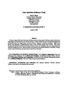
shapes from the latest drawn one and follow the reverse input sequence until one of the four conditions is met: 1. No ungrouped shapes available, 2. d > dmax, 3. σ > σmax, or 4. The bounding box of SG is bigger than a given threshold. Thus the ultimate SG is the shape group we guess for the user-intended shape. Fig.3 illustrates an example of primitive shapes grouping. The red line segment is the latest input shape, and it can be grouped together with two quadrangles. The circle cannot be grouped in because it would make the combined shape imbalanced (the σ value would exceed the threshold).
Fig.3. Primitive shapes grouping
3.3 Partial Structural Similarity Calculation After primitive shape grouping, the combined shape group can also be regarded as a composite object. This object (the source object) and each candidate object (the destination object) in the database are then compared for similarity assessment. Since the inputted shape might be in an incomplete form, the similarity is not symmetric between the source and destination objects. It is a “partial” similarity measured from the source to the destination objects. For example, if the source object (an incomplete object) is a part of the destination object (a complete object), we think they are highly similar because the source object can be completed later. However, if the source object contains certain components that do not exist in the destination object, we think their similarity should be very low, no matter how similar other corresponding parts are. First, we normalize the source object and the candidate object into a square of 100*100 pixels. Then we calculate the partial structural similarity in two stages. In the first stage, primitive similarity is only measured based on matched primitive shapes. In the second stage, these matched primitive shapes are removed from both the source and the designation objects. More elaborate shape similarity is then adjusted according to the similarity of the topological structures of the remained parts. 3.3.1 Similarity between Primitive Shapes An intuitive way to calculate the similarity between the source object and the destination object is to compare their components one-by-one based on identical shape types and relative positions. The overall similarity can be acquired through a weighted sum of similarity of their matched components. We define Average Point Shifting (APS) for two primitive shapes if their types are identical through the following rules:
1. If both are line segments, denote them as P1-P2 and P3-P4. The APS of two line segments is defined as APS L =
1 ( Min( Dis ( P1 , P3 ) + Dis ( P2 , P4 ), Dis ( P1 , P4 ) + Dis ( P2 , P3 )) 2
(4)
2. If both are arc segments, denote them as P1-P12-P2 and P3-P34-P4, where P12 and P34 are the middle point of an arc. The APS of two arc segments is defined as APS A =
1 ( APS L + Dis ( P12 , P34 )) 2
(5)
3. If both are n-polygons (n is the number of vertexes), denote their vertex lists (in the same traversal order) as P0, P1, … Pn-1 and Q0, Q1, … Qn-1 respectively. The APS between two polygons is defined as n −1
APS P = Min ( j =0
1 n −1 ∑ Dis ( Pi ,Q (i + j ) mod n )) n i =0
(6)
4. If both are ellipses, the APS is defined as the APSP between their bounding boxes. The partial structural similarity between two composite objects is then defined based on APS. Denote the component set of the source object as S, which has m components S1, S2, …Sm. Denote the component set of the destination object as D, which has n components D1, D2, …Dn. If m=0, the similarity is defined as 1. If m>n, the similarity between them is 0. Otherwise (n≥m), we create a mapping j form [1, m] to [1, n], which satisfies the following two conditions: 1. For each i ∈[1, m], Si and Dj(i) are of the same shape type. 2. For i1, i2∈[1, m] and i1≠ i2, j(i1)≠j(i2). Enumerate all these possible mappings and denote them as a set J. The partial structural similarity between the source object and the destination object can be obtained by
Sim prim ( S , D ) = Max (1 − j∈J
1 m APS ( S i , D j (i ) ) ∑ 100 2 ) m i =1
(7)
where 100 2 is the length of the diagonal of the normalized area. 3.3.2 Similarity between Object Skeletons Admittedly, different users may have different opinions in decomposing a composite object into primitive shapes. Even the same user may change his ideas from time to time. E.g., for the composite graphic object called “envelope”, a user may input it by drawing a pentagon and a triangle. However, he may also input it by drawing a pentagon and two line segments. See Fig.4 for illustrations of two ways to draw the “envelope”. Although the ultimate combined objects look totally the same, they cannot match each other through the previous strategy presented in Sect. 3.3.1. Moreover, it is extremely difficult to enumerate all the possible combinatorial ways to draw a
composite graphic object, in both spatial and temporal considerations. Hence, we also need to find other ways to measure similarity between two composite objects. =
+
=
+
+
Fig.4. A composite graphic object may be drawn in several different ways
Object skeleton is a graph we use to represent the topological structure of the composite object. In order to acquire the skeleton of the object, we first generate an initial candidate skeleton and then merge redundant nodes and edges to obtain the ultimate one. See Fig.5 for illustration. Node generation is first done based on the following rules: 1. All vertices of polygons are candidate nodes, such as Point 1~7. 2. All end points of line and arc segments are candidate nodes, such as Point 8 and 9. 3. The middle points of arc segment are candidate nodes. 4. All of the cross points (of two different primitive shapes) are candidate nodes, such as Point 10 and11. 1
2
1
2 5
5 8
9 10
4 (a) the destination object in the database (some primitive shapes has been removed)
(b) the source object that the user has input (some primitive shapes has been removed)
6
10
11 7
3
(c) the initial skeleton for (b)
11
4
3 (d) the ultimate skeleton for (b)
Fig.5. Object skeleton acquisition
After nodes generation, these candidate nodes divide the polygon and line segment into several pieces. Each piece can be logically represented by an edge (a line segment). If a node’s distance to an edge is under a threshold, we move this node on the edge (choose the most nearest point on the line segment to replace the node) and split the edge into two pieces. E.g., in Fig.5 (c), node 5 splits the edge between node 1 and 2 into two pieces. After getting the initial skeleton, those nodes that are close enough are merged. Edges must be correspondingly adjusted to adapt to the new nodes. All fully overlapping edges should be merged into one. E.g., in Fig.5 (c), node 4 and 6 are combined into node 4. And node 7and 3 are combined into node 3. Thus, the edge between node 6 and 7 is then eliminated. After these processes, we can get the ultimate object skeleton, as illustrated in Fig.5 (d). The object skeleton is represented by a graph consisting of a node set and an edge set. The similarity between object skeletons is calculated based on their topological structures. Denote the node set of the source object skeleton as NS, which has m elements. Sort these nodes according to the sum of their x coordinate and y coordinate
descendent, denote them as NS1, NS12, … NSm. Denote the node set of the destination object skeleton as ND, which has n elements. Use the similar way sort them in a list, denote them as ND1, ND12, … NDn. Define the edge set of the source object as ES and the edge set of the destination object as ED. Define logical edge set of the destination object LED={(i1, i2)| (NDi1, NDi2)∈ED, i1, i2∈[1, n]}. If m=0, the similarity is defined as 1. If m>n, the similarity between these two skeletons is 0. Otherwise (n≥m), create a mapping j from [1, m] to [1, n] which satisfies the following two conditions. 1. For each i1, i2∈[1, m] and i1≠i2, j(i1)≠j(i2). 2. For each i1, i2∈[1, m] and i10 and w1+w2+w3=1. The computational complexity of this algorithm depends on ε. If ε=0, the number of all possible mapping is C nm . If ε≥n, the m
number of all possible mapping is Pn . Hence, the computational complexity of this m
algorithm is between C nm and Pn . The larger ε is, the larger the computational cost is, and more accurate result can be obtained. 3.3.3 The Overall Similarity Calculation The computation complexity of similarity calculation between object skeletons is very high for a real-time system. Hence, we must reduce the node number to save calculation time. We find users have common senses to group some parts of a composite graphic object into one primitive shape. For instance, users usually draw some special primitive shape types (E.g., ellipse, hexagon, etc.) in a single stroke and seldom divide them into pieces (multiple strokes). The same situation is for some isolated primitive shapes, which do not have intersection with other parts of the object. These primitive shapes can be separated from other strokes of both the source and the
destination objects and first compared by our primitive shape comparison strategy. Then, the remained parts of both objects can be compared through our object skeleton comparison strategy. Thus the node number of object skeleton can be much reduced. Denote the source object as S and the destination object as D. Denote the separated primitive shapes of S and D as Sprim and Dprim respectively. Denote the remained parts of S and D are Srem and Drem respectively. The overall similarity between S and D is a linear combination of the similarities between Sprim and Dprim and that of Srem and Drem, as defined in Eq. (12). 0 , if Sim prim ( S prim , D prim ) = 0 or Simk (S rem , Drem ) = 0 Sim ( S , D) = otherwise k1 Sim prim (S prim , D prim ) + k 2 Simk (S rem , Drem ) ,
(12)
where k1, k2>0 and k1+ k2=1. 3.4 The User Interface and Relevance Feedback We implement the proposed approach in our SmartSketchpad [1] system. After only a few components of a composite object are drawn, the similarities between the input source object and those candidates in the database are then calculated using the partial structural similarity assessment strategy. The most similar objects are displayed in a ranked candidate list (according to the descending order of similarities) in the smart toolbox for the user to choose. If the user cannot find his/her intended shape, he/she can continue to draw other components until the intended one appears in the list. In order to avoid too much intrusive suggestion of composite shapes of low similarity, only the first ten objects whose similarities are above a threshold (which is 0.3 currently) are displayed in the smart toolbox for suggestions. The smart toolbox will not give any suggestion if less than two components are drawn. E.g., if a user wants to input a graphic object called “bear”, he/she can first draw its face and an ear by sketching two circles. But the intended object does not appear in the smart toolbox. Then the user continues to draw its right ears by sketching a smaller circle. This time, the wanted object appears and is ranked as the 5th in the smart toolbox for selection. If the user did not notice this, he/she can continue to draw its left eye by sketching a line segment. # 2
Input
Sim 0.407362
Rank 12
3
0.447857
5
4
0.852426
1
ID: # of input components Sim: Similarity of the intended object
Candidates sorted in descending similarity
Input: The input components Rank: Rank of the intended object
Fig.6. Input a composite graphic object by sketching a few constituent primitive shapes
This time, only three objects are listed and the wanted object is ranked as the first in the smart toolbox. See Fig.6 for illustration. However, the partial structural similarity
calculation strategy we have proposed is not perfect yet. During the drawing processes, irrelevant objects may obtain higher ranks in the object list. Sometime, users have to draw the intended object completely so that it could be seen in the list. Or, even after the entire object is drawn, it still does not appear in the smart toolbox. In this case, the user has to click the “more” button continually to find his/her intended object. In order to avoid such situation, relevance feedback is employed to improve both input efficiency and accuracy. Because each user has his/her drawing style/preference, a specific user tends to input the same object through a list of components of fixed constitution (e.g., two ellipses and a triangle) and fixed input time sequence (e.g., ellipse-triangle-ellipse). Hence, the input primitive shape list offers much more information that we have not utilized in our partial structural similarity calculation. Each time when the user drags an object from the smart toolbox, the current grouped input primitive shape list will be saved as a “word” index for this intended object with a probability. E.g., a list rectangle-triangle may be used for index of “envelope” and “arrow box”. The probability can be easily obtained from the relative times when the intended object is selected for this “word”. Hence, for an inputted source object and a candidate object in the database, we not only can acquire their shape similarity using the partial structural similarity calculation strategy, but also can acquire the probability (initially, all possibilities are set to 0) that the candidate object is just the intend one. We linearly combine them with different weights to obtain a new metric for similarity comparison. Therefore, if a user always chooses the same candidate object for a specific input primitive shape sequence, the probability of this candidate object must be much higher than that of other candidate objects. Obviously, through this relevance feedback strategy, the intended object will obtain a higher rank than before.
4 Performance Evaluations In this experiment, we created 97 composite graphic objects for experimentation in SmartSketchpad. All these objects are composed of less than ten primitive shapes, as shown in Fig.7. The weights and thresholds we used are ε=20, w1=0.4, w2=0.3, w3=0.3, k1=k2=0.5.We randomly selected 10 objects (whose ID is 73, 65, 54, 88, 22, 5, 12, 81, 18, and 76) and draw these objects as queries. We recorded the intended object’s rank variation together with the drawing steps. Results of four objects are shown in Fig.8. The horizontal coordinate is the input steps. In each step, only one component is drawn until the object is properly finished. The vertical coordinate is the rank of the intended object. In most cases, the intended object will appear in the smart toolbox (ranked in the first 10) after only a few components are drawn. Take Object 73 as an example. The user can input this object in 6 steps. After four components are drawn, the intended object’s rank is 4. Thus the user can directly drag it form the smart toolbox. Averagely (of the ten objects we have tested), after 85.7% components of the intended object are drawn, it will be shown as the first one in the smart toolbox. In order to see it in the smart toolbox (top 10), only 67.0% of the intended object needs to be drawn. And the ratio is 68.7% for top 5 and 72.0 for top 3. The user does not need to draw the complete sketch for a composite graphic object. Only a few sketchy
components are sufficient for the system to predict the user’s intent. Hence, this user interface provides a natural, convenient, and efficient way to input complex graphic objects.
Fig.7. The composite graphic objects we have created for experimentation 100
100
80
80
60
60
40
40
33
20
38
12
4
3
1
4
5
1
1 2
6
3
4
100
80
80
60
60
6
1 7
40
30
25
20 2
0 2
5
Object 54
100
20
25
0
Object 73
40
25
20
0 2
61
3
1 4
Object 76
1 5
10
0 2
3
2 4
1 5
1 6
Object 5
Fig.8. The intended object’ ranks (vertical axes) and input steps (horizontal axes)
5 Summary We proposed a novel user interface to input composite graphic objects by sketching only a few of their constituent simple/primitive shapes. The inputted shape’s
similarities to those objects in the database are updated in the drawing process and those promising composite objects are suggested to the user for selection and confirmation. By doing so, the user is provided with a natural, convenient, and efficient way to input composite graphic objects and can get rid of the traditional graphic input interface based on menu selection and this user interface is especially suitable for small screen devices.
6 Acknowledgement The work described in this paper was fully supported by a grant from City University of Hong Kong (Project No. 7100247) and partially supported by a grant from National Natural Science Foundation of China (Project No. 69903006).
7 References 1. Liu, W., Qian, W., Xiao, R., and Jin, X.: Smart Sketchpad—An On-line Graphics Recognition System. In: Proc. of ICDAR2001, Seattle (2001) 1050-1054 2. Zeleznik, R.C., Herndon, K.P., Hughes, J.F.: SKETCH: An Interface for Sketching 3D Scenes. In: SIGGRAPH96, New Orleans (1996) 163-170 3. Gross, M.D., Do, E.Y.L.: Ambiguous Intentions: A Paper-like Interface for Creative Design. In: Proc. of the 9th Annual ACM Symposium on User Interface Software and Technology, Seattle, WA (1996) 183-192 4. Albuquerque, M.P., Fonseca, M.J., Jorge, J.A.: Visual Language for Sketching Document. In: Proc. IEEE Sym. on Visual Languages (2000) 225-232 5. Fonseca, M.J., Jorge, J.A.: Using Fuzzy Logic to Recognize Geometric Shapes Interactively. In: Proc. 9th IEEE Conf. on Fuzzy Systems, Vol. 1 (2000) 291-296 6. Arvo, J., Novins, K.: Fluid Sketches: Continuous Recognition and Morphing of Simple Hand-Drawn Shapes. In: Proc. of the 13th Annual ACM Symposium on User Interface Software and Technology, San Diego, California (2000) 7. Sklansky, J., Gonzalez,V.: Fast Polygonal Approximation of Digitized Curves. Pattern Recognition 12 (1980) 327-331 8. Graham, R.L.: An Efficient Algorithm for Determining the Convex hull of A Finite Planar Set. Information Processing Letters 1(4) (1972) 132-133 9. Esther, M.A., et al.: An Efficient Computable Metric for Comparing Polygonal Shapes. IEEE Trans. on PAMI 13(3) (1999) 209-216 10. Vapnik, V.: The Nature of Statistical Learning Theory. Springer-Verlag, New York (1995)