Software Cost Estimation Models and Techniques: A ...

International Journal of Engineering Research & Technology (IJERT) ISSN: 2278-0181 Vol. 3 Issue 2, February - 2014

Software Cost Estimation Models and Techniques: A Survey 1

Yansi Keim, 1Manish Bhardwaj, 2Shashank Saroop, 2Aditya Tandon

Department of Information Technology Ch. Brahm Prakash Government Engineering College, Jaffarpur, New Delhi-110073  Abstract— Software products are said to be feasible if they are developed within the budget constraints. Prior to making software product it’s imperative to predict the software development cost. Practitioners have expressed concern over their inability to accurately estimate costs associated with software development. This concern has become even more pressing as costs associated with development continue to increase. As a result, considerable research attention is now directed at gaining a better understanding of evaluating software cost estimating tools. This paper summarizes software cost estimation models: COCOMO II, COCOMO, PUTNAM, STEER and ESTIMACS based on the parameters implement ability, extensibility, flexibility and traceability and techniques used to estimate software costs.

I. INTRODUCTION

Software cost estimation model is an indirect measure, which is used by software personnel to predict the cost of a project. They are used for the number of purposes. It includes:  Budgeting   Overall estimate has to be accurate, the most desired capability. Hence initial efforts are directed in predicting budget for the software product.    Tradeoff and risk analysis   An important additional capability is to illuminate the cost and schedule sensitivities of software project decisions (scoping, staffing, tools, reuse, etc.).    Project planning and control   An additional potential is to provide cost and schedule breakdowns by component, stage and activity.    Software improvement investment analysis Strategies such as tools, reuse, and process maturity benefit the development process of software.[1]  This paper has been divided into five sections. Initial being Introduction, Section II pertains to surveying of various Cost

IJERTV3IS20384

Economy of s/w development would reduce the current difficulties of software production resulting in cost overruns or even project cancellations. Just like in any other field, the field of software engineering cost models has had its own pitfalls. The fast changing nature of software development has made it very difficult to develop parametric models that yield high accuracy for software development in all domains. S/w development costs hikes abnormally and practitioners continually express reckon over their incapability to accurately predict the costs involved. S/w models constructively explain the development life-cycle and accurately predict the cost of developing a software product [2]. Many s/w estimation models have evolved in the last two decades based on the pioneering efforts by the researchers. Mostly being proprietary models cannot be compared and contrasted as far as the model structure is concerned [3]. Theory or experimentation determines the functional form of these models. These are:

IJE RT

Index Terms— Software Cost Estimation Model, Software Development, Software Development Cost, Development Life Cycle, KLOC (Kilo Lines of Code), function count (FC), S/w (Software), KDSI (Kilo Delivered Source of Instruction), AT (Algorithmic Technique), NAT (Non-Algorithmic Technique)

Estimation Models. Section III regards to surveying distinct cost estimation techniques. Section IV defines comparative analysis of various models on the basis of certain parameters. Finally, Section V summarizes and tells about future scope for the same. Section VI is References.  II. COST ESTIMATION MODELS

1. COCOMO 81 1(a) Basic COCOMO COCOMO is an acronym used for Constructive Cost Model. It was first published in 1981 book Software Engineering Economics by Barry Boehm. It gives the magnitude of cost of project due to the ease of openness of model. It is meant for relatively small projects as a very few cost drivers are associated with it. Its supportive when the team size is small, i.e. small staff. It ’ s good for quick, early, rough, order of magnitude of software costs, but its accuracy is necessarily limited because of its lack of factors to account for difference in hardware constraints, personnel quality and experience, use of modern tools and techniques and other project attributes are known to

www.ijert.org

1763


have a significant influence on s/w costs. EFFORT = a* (KDSI)

design, etc) of the software engineering process.

b

2. COCOMO-II

The value of constants a & b depend on the project type. The estimated number of delivered lines of code for the project accounts for the KLOC. Basic COCOMO has three types of modes which are following [4]:Organic Mode: Relatively small, simple s/w project in which a small teams with good application experience. Efforts, E and Development, D are:E= 2.4*(KLOC) 0.38 D=2.5*(E)

1.05

Semi-detached Mode: An intermediate s/w projects in which teams with mixed experience E = 3.0* (KLOC) D=2.5*(E)

1.12

0.35

E = 3.6* (KLOC) D=2.5*(E)

1.20

0.32

1(b) Intermediate COCOMO

a.

The Application Composition model is worn to approximate effort and schedule on projects that use Integrated Computer Aided Software Engineering tools for rapid application development. It is based on Object Points (Object Points are a tally of the screens, reports and 3 GL language modules developed in the application). b. The Early Design Model involves the investigation of substitute system architectures and concepts of operation. c. The Post-Architecture Model is used when apex level design is complete and thorough information about the project is accessible and as the name suggests, the software architecture is sound defined and well-known. It accounts for the intact development life-cycle and is a exhaustive extension of the Early-Design model. This is a lean-to intermediate COCOMO model and defined as:-

IJE RT

Embedded Mode: A s/w project that must be developed within a set of tight h/w, s/w and operational constraints

The COCOMO II research effort was started in 1994 at USC. Its major focus on non-sequential and rapid development process models, reengineering, reuse driven approaches, object oriented approaches, etc. It is a cumulative result of three variants, Application composition model, Early design model, and Post architecture model [5].

EFFORT = 2.9 (KLOC)

1.10

3. PUTNAM MODEL (SLIM)

It evaluates software development effort as a function of program size and set of cost drivers that include subjective examination of the products, hardware, personnel and project attributes. It is used for medium sized projects. The cost drivers are intermediate to basic and advanced COCOMO. Product reliability, database size, execution and storage are function of cost drivers. Team size is medium. The intermediate COCOMO model takes the form:

SLIM (Software Life Cycle Model) is based on Putnam’s study in terms of Rayleigh distribution of project personnel level versus time. It chains most of the popular size estimating methods including ballpark techniques, source instructions, function points, etc. It estimates project effort, schedule and defect rate. Record and analyze data from formerly completed projects which are then used to standardize the model [3]. If data are not obtainable then a set of questions can be answered to get values of MBI and PF from the presented database. Productivity, P, is the ratio of software product size S and development effort E is that is

EFFORT = a* (KLOC) b * EAF

P=

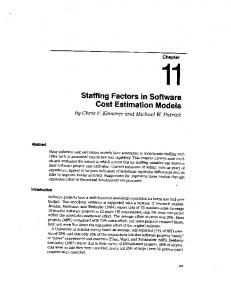
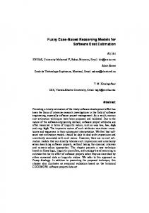
Here effort in person-months and KLOC is the estimated number of delivered lines of code for the project. The Rayleigh curve [2] is accustomed to define the distribution of effort which is modeled by the differential Equation

1(c) Detailed COCOMO It is used for large sized projects. Requirements, analysis, design, testing and maintenance determines the cost drivers, here. Team size is large. The detailed COCOMO Model inculcates all features of the intermediate version with an assessment of the cost driver’s effect on each step (analysis,

IJERTV3IS20384

www.ijert.org

1764


a product offered by Galorath, Inc. of El Segundo, California. This model is based on the original Jensen model [Jensen1983], and has been on the market since last 15 years. The scope of the model is broad. It covers all phases of the project life-cycle, from early specification all the way through design, development, delivery and maintenance. It facilitates extensive sensitivity and trade-off analyses on model input parameters. It organizes project elements into work breakdown structures for suitable planning and control and displays project cost drivers. The model allows the interactive scheduling of project elements on Gantt charts. Builds estimates upon a sizable information base of existing projects [2].

Fig. 1: The Rayleigh Model

4. ESTIMACS

a. b. c. d. e.

IJE RT

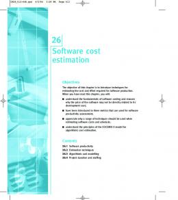
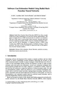
It is a proprietary system which is used in critical flight s/w [7] and was marketed by Management and Computer Services (MACS). ESTIMACS stresses impending the evaluating task in business terms. Rubin has recognized six vital proportions of estimation and a map presenting their interactions, all the way from what he calls the gross business terms through to their impact on the developer’s protracted term projected portfolio mix. [3]The significant estimation dimensions are: effort hours, staff size and deployment, cost, hardware resource requirements, risk, portfolio impact..

III.

COST ESTIMATION TECHNIQUES

A. Algorithmic Techniques Algorithmic methods use a formula to calculate the software cost estimate. The formula is developed from models which are created by combining related cost factors. In addition, the statistical method is used for model construction.

Fig. 2: Rubin’s map of relationship of estimation dimensions

5.SEER-SEM SEER-SEM is System Evaluation and Estimation of Resources,

IJERTV3IS20384

The algorithmic method is designed to provide some mathematical equations to perform software estimation. These mathematical equations are based on research and historical data and use inputs such as Source Lines of Code (SLOC), number of functions to perform, and other cost drivers such as language, design methodology, skill-levels, risk assessments, etc. The algorithmic methods have been largely studied and many models

www.ijert.org

1765


have been developed, such as COCOMO models, Putnam model, and function points based models.

small software components and the interactions. The leading method using this approach is COCOMO's detailed model.

Function Point Analysis

iii. Estimating by Analogy

The Function Point Analysis is another method of quantifying the size and complexity of a software system in terms of the functions that the systems deliver to the user. A number of proprietary models for cost estimation have adopted a function point type of approach, such as ESTIMACS and SPQR/20. This is a measurement based on the functionality of the program and was first introduced by Albrecht [8]. The total number of function points depends on the counts of distinct (in terms of format or processing logic) types.

Estimating by analogy means comparing the proposed project to previously completed similar project where the project development information id known. Actual data from the completed projects are extrapolated to estimate the proposed project. This method can be used either at system-level or at the component-levels. The estimating steps using this method are as follows: a. Find out the characteristics of the proposed project.

There are two steps in counting function points:

ii.

Counting the user functions:- The raw function counts are arrived at by considering a linear combination of five basic software components: external inputs, external outputs, external inquiries, logic internal files, and external interfaces, each at one of three complexity levels: simple, average or complex. The sum of these numbers, weighted according to the complexity level, is the number of function counts (FC). Adjusting for environmental processing complexity:- The final function points is arrived at by multiplying FC by an adjustment factor that is determined by considering 14 aspects of processing complexity.

B. Non-Algorithmic Techniques Non-algorithmic methods do not use a formula to calculate the software cost estimate. i. Top-Down Estimating Method Top-down estimating method is also called Macro Model. Using top-down estimating method, an overall cost estimation for the project is derived from the global properties of the software project, and then the project is partitioned into various low-level mechanism or components. The leading method using this approach is Putnam model. This method is more applicable to early cost estimation when only global properties are known. In the early phases of the software development, it is very useful because there is no detailed information available. ii. Bottom-Up Estimating Method Using bottom-up estimating method, the cost of each software components is estimated and then combines the results to arrive at an estimated cost of overall project. It aims at constructing the estimate of a system from the knowledge accumulated about the

IJERTV3IS20384

b. Select the most similar completed projects whose characteristics have been stored in the historical data base. c. Find out the estimate for the proposed project from the most similar completed project by analogy.

IV.

COMPARATIVE ANALYSIS OF VARIOUS MODELS ON THE BASIS OF CERTAIN PARAMETERS

IJE RT

i.

COCOMO 81 or COCOMO I model published in 1981. In [2], Barry Boehm described the capabilities of COCOMO 81 from simply providing cost estimation capability to sensitivity analysis and trade-off analysis. The reports in [3] tell us the model being entirely transparent; its openness shows how it works. The drivers are helpful to understand the factors affecting project costs. However the shifting needs from mainframe overnight batch processing to real time application, strenuous effort in building s/w for reusing, new system development including the off-the-shelf component, spending as much effort on designing, managing the s/w software development process once spent creating the s/w product, application generation programs, object oriented approaches. The model’s success greatly requires historical data, but it might not be present every time. The COCOMO-II came into existence [2] when needs mentioned above arose. Joint efforts of USC-CSE (University of California, Center for Software Engineering) and the COCOMO II Project Affiliate Organizations the COCOMO II model was presented in 1995. It supported updated project database [7]. The strategy maintained focused upon preserving the openness of previous version.

SLIM s/w cost estimation model has not been widely accepted due to certain limitations. Why it has been initially accepted is given below: One of the key advantages to this model is the

www.ijert.org

1766


simplicity with which it is calibrated. Most software organizations, regardless of maturity level can easily collect size, effort and duration (time) for past projects. Process Productivity, being exponential in nature is typically converted to a linear productivity index an organization can use to track their own changes in productivity and apply in future effort estimates. [2] Why this model is not widely accepted? One significant problem with the PUTNAM model is that it is based on knowing, or being able to estimate accurately, the size (in lines of code) of the software to be developed. There is often great uncertainty in the software size. It may result in the inaccuracy of cost estimation. The error percentage of SLIM, a Putnam model based method, is 72.87%. The ESTIMACS model was developed by Howard Rubin of Hunter College as an outgrowth of a consulting assignment to Equitable Life. It is a proprietary system and, at the time the data were collected, was marketed by Management and Computer Services (MACS). Since it is a proprietary model, details, such as the equations used, are not available. The model does not require

Current Version: SEER for Software Version 7.3 is a vast improvement over the original implementation, representing perhaps the first time that any version of SEER could be integrated to support all phases of a project's lifecycle. The size of the software has grown to over 200,000 source lines of code and shifted from simply a means to generate work estimates through parametric modeling to a system that buttresses those results with simulation-based probability and over 20,000 historical cases to draw conclusions from.

IJE RT

SLOC as an input, relying instead on “Function-Point-like” measures. The research in this paper is based on Rubin’s paper from the 1983 IEEE conference on software development tools and the documentation provided by MACS [ZO, 221. The 25 ESTIMACS input questions are described in these documents. The ESTIMACS average error is 85 percent, which includes some over and some under estimates, and is the smallest average error of the four models. [7]

has undergone numerous upgrades, keeping up with changing technology, adapting to better meet the needs of the customer, and altering the model to achieve more precise estimates. For example, the 1994 release of SEER-SEM version 4 included major enhancements to the core math behind the model, handling the realities of projects rather than just a Rayleigh curve approximation, as well as dozens more knowledge bases and the latest research in software science and complexity metrics. 2003 saw SEER-SEM add significant new features such as Goal Setting and Risk Tuning. Both features operated as their names suggest with Risk Analysis allowing project managers to make changes to estimates and Goal Setting allowing for projects to not only be estimated, but also to be managed. Version 6 of SEER for Software was the first to be fully COM-enabled, allowing SEER to both input and output through various Microsoft products, such as Excel. Version 7 included better handling of projects that stretch beyond their optimal effort. [9]

The original SEER-SEM has also branched into:

There is a brief discussion given below how the SEER-SEM model gone through its development stages and which version is currently in use. SEER-SEM model has made its unique way in software cost estimation process.



Version 1.0: In 1988, Galorath Incorporated began work on the initial version of SEER-SEM which resulted in an initial solution of 22,000 lines of code. SEER-SEM version 1.0 was released on 13 5.25" floppy disks and was an early product running on Windows version 2. Designing SEER-SEM for Windows was considered risky as the operating system had yet to establish itself as a viable competitor to the current dominant OS, Microsoft's MS-DOS. However, the adoption of a Windows-based format proved to be worthwhile, allowing SEER-SEM to offer a much more intuitive user interface than would have otherwise been available in MS-DOS. Galorath chose Windows due to the ability to provide a more graphical user environment, allowing more robust management tradeoffs and understanding of what drives software projects. Next Versions: Since that initial release in 1988, SEER-SEM



IJERTV3IS20384



www.ijert.org



SEER for Information Technology – SEER-IT  – a version of SEER created to aid IT professionals estimates the design, build, and maintenance of information technology infrastructures and service management projects. 



SEER for Hardware, Electronics, & Systems – SEER-H – a version of SEER designed to aid in the life-cycle cost estimation of any type of hardware, electronics or system.  



SEER for Manufacturing – SEER-MFG – a version of SEER tailored for estimating the detailed production costs of manufacture, covering a wide range of state-of-practice manufacturing process knowledge.[10] 

1767


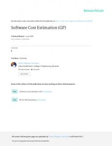
S. No.

Model Name

01.

ESTIMACS

Howard Rubin

02.

PUTNAM‟ s S/w Life Cycle Model(SLIM)

03. 04

05.

Author

Year of Publishing

Parameters Technique Used Extensibility

Flexibility

√

√

1970

Function Point (AT)

L.H. Putnam,

1978

Ballpark Technique (NAT), Function Point (AT),

COCOMO 81[3][4][5][6]

Barry Boehm

1981

SLOC‟ s, KDSI

√

SEER-SAM

Galorth

1983

Top-down, bottomup

√

1995

Object Point, Function Point, SLOCs, KSLOC

COCOMO II

USC-CSE & COCOMO II Project Affiliate Organizations

Traceability

√

Easy to Implement Being proprietary, accessibility is less

√ √

√

√

Suitable for SLC over 2,00,000

√

√

Suitable for large size projects

Table 1 Comparison of various Cost Estimation Models

FUTURE SCOPE

]REFERENCES Ashita Malik, Varun Pandey, Anupama Kaushik et al.(2013), “Analysis of Fuzzy Approaches for COCOMO II”, Vol-6, India, pp 68-75 [2] Barry Boehm, Chris Abts, Sunita Chulan et al. (2000), “Software Development Cost Estimation Approaches”, Annuals of Software Engineering, 10, pp 177-205 [3] Barry Boehm, Chris Abts, Sunita Chulani et. al., “Software Development Cost Estimation Approaches- A Survey”, IBM Research [4] Roger S. Pressman, 1997 – Software Engineering – A Practitioner‟ s Approach, Fourth Edition; http://groups.engin.umd.umich.edu/CIS/course.des/cis525/js/f00/gamel/ help.html [5] Sunita Devnani-Chulani et. al(May 1999), “Bayesian Analysis of Software Cost and Quality Models” [6] Astha Dhiman, Chander Diwaker et. al(2013), “Optimization of COCOMO II Effort Estimation using Generic Algorithm” [7] Raymond Madachay, Barry Boehm et. al(2008), “Comparative Analysis of COCOMO II, SEER-SEM and True-S Software Cost Models” [8] Sweta Kumari, Shashank Pushkar et. Al(2013), “Performance Analysis of Software Cost Estimation Methods: A Review” [9] Galorath, D & Evans M. (2006) Software Sizing, Estimation, and Risk Management ISBN 0-8493-3593-0

IJE RT

V.

Here, we have carried out the comparative systematic study of some software cost estimation models in conjunction with their relevant techniques. Although, it would be awfully difficult to say which model is preeminent as it is vastly based on the size of software and certain other factors. But, largely COCOMO-II is hugely used and has a broad prospect too.

Thus, we would like to carry out our future study on the same. VI. ACKNOWLEDGEMENT

This paper has come out as a successful work product due to the throughout support of our well-regarded teacher Mr. Gulzar Ahmad (Assistant Professor).

IJERTV3IS20384

[1]

www.ijert.org

1768