Solutions to Exercises in Chapter 3 - Routledge

ANSWERS TO EXERCISES IN

PROGRAMMING AND SCHEDULING TECHNIQUES 2nd edition

Thomas E. Uher Adam Zantis

This edition published 2011 by Spon Press 2 Park Square, Milton Park, Abingdon, Oxon, OX14 4RN Simultaneously published in the USA and Canada by Spon Press 270 Madison Avenue, New York, NY 10016 Spon Press is an imprint of the Taylor & Francis Group, an informa business © 2011 Thomas E Uher and Adam Zantis The right of Thomas E Uher and Adam Zantis to be identified as authors of this work has been asserted by them in accordance with sections 77 and 78 of the Copyright, Designs and Patents Act 1988.

All rights reserved. [No part of this book may be reprinted or reproduced or utilised in any form or by any electronic, mechanical, or other means, now known or hereafter invented, including photocopying and recording, or in any information storage or retrieval system, without permission in writing from the publishers. The publisher makes no representation, express or implied, with regard to the accuracy of the information contained in this book and cannot accept any legal responsibility or liability for any errors or omissions that may be made.

ANSWERS TO EXERCISES IN PROGRAMMING AND SCHEDULING TECHNIQUES

2nd edition

Thomas E. Uher Adam Zantis

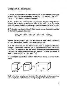
FOREWORD This Answers to Exercises document supplements the Programming and Scheduling Techniques textbook. It contains worked solutions to exercises set out in most chapters of the textbook. The exercises have been carefully formulated to improve your comprehension of important topics explained in the textbook and to enable you to self-test your knowledge. Upon accessing Answers to Exercises on the Spon Press website, you may peruse this document, download it or even print it free of charge. The most effective way of using Answers to Exercises is for you to solve or attempt to solve individual problems first before looking up the answers. We trust you will find Answers to Exercises a useful supplement to the textbook. We are confident that it will improve your understanding of the programming and scheduling techniques introduced in the textbook, and make your study much easier and more enjoyable.

T.E. Uher A. Zantis

CONTENTS ANSWERS TO EXERCISES IN CHAPTER 3

5

ANSWERS TO EXERCISES IN CHAPTER 4

9


15


18


29


40


44


47

ANSWERS TO EXERCISES IN CHAPTER 3 (pp ) Solution to exercise 3.1 Precedence schedule

A

C

G

D

F

M

E

L

N

P

J

O

H

B

K

1

Solution to exercise 3.2 Precedence schedule

A

B

C

G

D

H

L

J

K

E

M

Q

N

P

F

O


B

A

C

D

E

H

J

F

G

N

L

K

2

M



3

Solution to exercise 3.6

4

ANSWERS TO EXERCISES IN CHAPTER 4 (pp...........) Solution to exercise 4.1 (a)

Solution to exercise 4.1 (b)

5

Solution to Exercise 4.2 (a)

Solution to exercise 4.2 (b)

A more even distribution of the total daily labour resource may be achieved by varying it or by splitting it. 6


Trade Contract

Activity

1

Formwork Contingency Reinforcement Concrete Conduits & cables Contingency Handrails Contingency A/C ducts Sprinkler pipes Contingency Plumbing stock Lift rails Contingency Bricks Mortar Windows Door frames Contingency Electrical Plaster Glazing Contingency Ceiling frames Wall & floor tiles Contingency Toilet partitions Contingency Plumbing fixtures Contingency Ceiling tiles Lights Contingency Lift doors Contingency Doors Vanity units Venetian blinds Mirrors Contingency Induction units Lift lobby finish Door hardware Contingency

2

3 4

5

6

7

8

9 10 11

12 13

14

Hoist Lifting Table No. of Cycle/ Activity loads/ time/ floor floor (min.) floor (hrs) 100 10% 40 170 5 10% 6 10% 20 10 10% 5 3 10% 15 10 7 3 10% 8 30 8 10% 4 20 10% 2 10% 2 10% 8 6 10% 17 10% 2 3 1 3 10% 2 12 4 10%

15

25 3 10 20 3 3 2 0 5 3 1 3 2 0 4 3 7 2 1 8 8 8 2 2 7 1 1 0 2 0 4 6 1 9 1 1 3 1 3 1 1 4 1 1

15 7 30 15 15 15 30 30 15 15 60 30 60 15 60 30 20 30 60 30 60 30 30 60 60 60 30 20 15

7

Total time/ floor (hrs)

Cumulat. time (hrs)

28

28

36

64

2

66

8

74

4

78

16

94

26

120

10

130

1

131

2

133

11

144

9

153

9

162

7

169

Cumulative Hoist Lifting Schedule Week Hoist time/week Cumulative hoist time No. in hours in hours

1 2 3 4 5 6 7 8 9 10 11 12 13 14 15 016 17 18 19 20 21 22 23 24 25 26 27 28 29 30 31 32 33 34

28 36 2 8 4 16 26 10 1 2 11 9 9 7

28 64 66 74 78 94 120 130 131 133 144 153 162 169 169 169 169 169 169 169 141 105 103 95 91 75 49 39 38 36 25 16 7 0

8

Hoist Lifting Schedule


1. The lift shaft will be built to level 3 (3 storeys) prior to installation of crane and will take 4 weeks to complete 2. The crane will be installed within the only Goods Lift 3. The jump form system will be installed using the crane and will take 3 weeks to complete 4. The structure will take 34 weeks to complete once the jump form is installed. There are approximately 329 load lifts required per floor with the average load weighing 4 tonnes and distance of 200 m Test Crane Speed = Loads/floor * no. of floors * cycle time per load = x, then convert to time scale Take Crane 1 for example = ((329 loads/floor * 34 floors * 12 min/load) / (60 min x 8 hrs))/ 6 days 5. The jump form system removal can take place after the structure is complete and will take 3 weeks to complete. 6. The roof plantroom is to be constructed from structural steel with the largest steel member weighing 5 tonnes and being located 45 m from the goods lift shaft. Test Crane load = tonne/metre * metre. Final load to be confirmed by crane supplier and structural engineer. Take Crane 1 for example = 8.25 tonne / 60 m * 45 m, then check with structural engineer & crane supplier 7. Heaviest permanent plant weighs 7 tonnes and is located 40 m from the goods lift shaft. Test Crane load = tonne/metre * metre. Final load to be confirmed by crane supplier and structural engineer. Take Crane 1 for example = 8.25 tonne / 60 metres * 40 m, then check with structural engineer & crane supplier 8. The crane can be removed after the final piece of plant is lifted into position and jump form removed.

9

Crane 1

Crane 2

Crane 3

28 days

28 days

28 days

5 days

3 days

3 days

18 days

18 days

18 days

NOT OK

OK

OK

47 weeks

35 weeks

31 weeks

18 days

18 days

18 days

OK

OK

NOT OK

6.2 t

5.4 t

OK

OK

4.5 t NOT OK

5.5 t

4.8 t

4.0 t

6 days

4 days

4 days

In selecting the appropriate crane for the project, all project information needs to be reviewed and a crane selected based on the crane speed, maximum reach, capacity at the maximum reach & average cycle time per lift. The project particular information should be tabulated as shown in the above table and each crane's ability to meet the project particular information should be analysed. The crane that can carry all heavy loads at the required distances and has the most efficient cycle time should then be selected. Based on the requirements of in the above exercise, Crane 2 appears to meet the requirements.

10

ANSWERES TO EXERCISES IN CHAPTER 5 (pp...........)


11


12


13

ANSWERS TO EXERCISES IN CHAPTER 6 (pp. ) Solution to exercise 6.1

14

15

16


17

18


19

20

21

22

23

Solution to exercise 6.4 (adapted from Burke, 1999, p 213) The EAC calculations are performed using the following equation: EAC = (ACWP/BCWP) x BAC Cases 1 2 3 4 5 6 7 8 9 10 11 12 13

BAC $10,000 $10,000 $10,000 $10,000 $10,000 $10,000 $10,000 $10,000 $10,000 $10,000 $10,000 $10,000 $10,000

BCWS $5,000 $5,000 $5,000 $5,000 $5,000 $5,000 $5,000 $5,000 $5,000 $5,000 $5,000 $5,000 $5,000

BCWP $5,000 $4,000 $5,000 $6,000 $4,000 $6,000 $4,000 $5,000 $6,000 $3,000 $4,000 $7,000 $6,000

ACWP $5,000 $4,000 $4,000 $4,000 $5,000 $5,000 $6,000 $6,000 $6,000 $4,000 $3,000 $6,000 $7,000

EAC $10,000 $10,000 $8,000 $6,667 $12,500 $8,333 $15,000 $12,000 $10,000 $13,333 $7,500 $8,571 $11,667

Case 1:

The project is on schedule and within cost budget.

Case 2:

The project is behind schedule but within cost budget.

Case 3:

The project is on schedule and under cost budget.

Case 4:

The project is ahead of schedule and under cost budget.

Case 5:

The project is behind schedule and over cost budget.

Case 6:


Case 7:


Case 8:

The project is on schedule but over cost budget.

Case 9:

The project is ahead of schedule and within cost budget.

Case 10:


Case 11:

The project is behind schedule but under cost budget.

Case 12:


Case 13:

The project is ahead of schedule but over cost budget.

24

ANSWERS TO EXERCISES IN CHAPTER 9 (pp............) Solution to exercise 9.1 The original schedule provides continuity of resource use for Trade A only (verify this by examining the earliest start and finish dates). Trade B is discontinuous as is Trade C. In Trade C, two activities ‘Level 4’ and ‘Level 5’ compete for the same resource.

With introduction of resource restraints, which ensure a logical progression of Trades A, B and C through the structure, the overlap between the activities ‘Level 4’ and ‘Level 5’ in Trade C was eliminated. However, the project duration was extended by 2 time units. Discontinuity in the use of the committed resources continues in Trades B and C. A clearer picture of the use of resources can be deduced by converting a critical path schedule to a MAC schedule.

25

The first three columns of MAC show the converted original schedule. The discontinuity in the use of the committed resources is clearly apparent as is the overlap between the activities ‘Level 4’ and ‘Level 5’ in Trade C. The next three columns show the converted schedule with the resource restraints. The planner can now adjust the schedule to eliminate or minimise discontinuity in the use of resources. The adjusted MAC is shown in the last three columns.

26

Solution to exercise 9.2 Alternative 1 Quantities of materials per floor and crew sizes have been calculated and are given in the table below. Activities

Quantities

Production rates

Setout ceiling grid Ceiling hangers @ 2m centres Ceiling frame Ceiling tiles Sprinkler heads @ 3m centres Light fittings @ 3m centres Aircon. registers @ 4m centres

16x11 = 176

Person hours

Crew size

8

Activity duration in hours 4

say 20

10

2

37

say 20 24

2

say 10 say 10 10

2

9x6 = 54

0.1 person hrs/hanger 50m/person hr 12.2 m2/person 3/person

9x6 = 54

6/person

9

7x4 = 28

3/person

10

(31x20m) + (41x30m) = 1,850m 30mx20m = 600m2

48 18

2

2

1 1

In this alternative, crew sizes have been kept at the maximum of 2 persons per crew per activity. To speed up ‘Ceiling fixing’, it is assumed that 2 crew of 2 persons each will work at the same time. The following MAC shows the arrangement of work for all the crews.

27

While the continuity of work of the ceiling fixing crews has been maintained, the other crews work discontinuously. The pattern of work of the ceiling fixing crews also changes substantially from one level to the next.

28

Alternative 2 The previous solution requires crews to move from floor to floor. Let’s try to work out a better solution by changing crew sizes. The adjusted MAC now provides a more satisfactory solution. Activities

Quantities

Production rates

Setout ceiling grid Ceiling hangers @ 2m centres Ceiling frame Ceiling tiles Sprinkler heads @ 3m centres Light fittings @ 3m centres Aircon. registers @ 4m centres

16x11 = 176

Person hours

Crew size

8

Activity duration in hours 4

say 20

20

1

37

10

4

48

12

4

18

10

2

2

9x6 = 54

0.1 person hrs/hanger 50m/person hr 12.2 m2/person 3/person

9x6 = 54

6/person

9

9

1

7x4 = 28

3/person

10

10

1

(31x20m) + (41x30m) = 1,850m 30mx20m = 600m2

29

30

Solution to exercise 9.3 The first truck will be unloaded in 54 minutes when the 8th pallet has been loaded with bricks. The cycle time of moving three pallets through the system is 21 minutes.

31


32

MAC schedule

Solution to Exercise 4.

33

Solution to exercise 9.5 Preliminary MAC schedule

34

Final MAC schedule

35

ANSWERS TO EXERCISES IN CHAPTER 10 (pp. ..............) Solution to exercise 10.1 With only one crew per activity, the total construction time in days per activity is calculated first. For example, the activity ‘A’ will take 4 days x 40 floors = 160 days. Durations of the other activities are given in the following table in the third column. Start and finish dates of the repetitive activities are given in columns 4 & 5. For example, the activity ‘D’, which is faster per cycle of work than its preceding activity ‘B’ will be scheduled from the end of the 40th completed activity ‘B’, which is day 164. The 40th activity ‘D’ will then be completed 3 days later or on day 167. The start of the 1st activity ‘D’ will then be 167 – 120 = 47. The LOB table Activity

Time duration in days

A B C D E F

4 4 6 3 8 4

Total construction time in days 160 160 240 120 320 160

Start of activity in days 0 4 8 47 14 178

Finish of activity in days 160 164 248 167 334 338

Let’s now add time buffer zones of 6 days and recalculate start and finish dates of the activities. The LOB table with buffer zones Activity

Time duration in days

A B C D E F

4 4 6 3 8 4

Total construction time in days 160 160 240 120 320 160

Start of activity in days 0 10 20 59 32 202

Finish of activity in days 160 170 260 179 352 362

The LOB schedule for the project in question is given below. 40 typical floors will be constructed in 362 days with the first floor fully completed on day 206.

36

The LOB schedule in the form of a graph

37

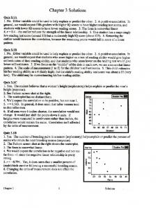
Solution to exercise 10.2 The production rates per week are calculated first from activity durations. They are given in the following LOB table in column 3. To achieve the required production output of 2 service stations per week, multiple crews are introduced to each activity, see column 4. Please remember that with multiple crews durations of activities per repetitive cycle will remain the same. Crews in each activity will work concurrently. For example, the activity ‘A’ will continue to take 3 weeks per service station, however, there will be 6 of these activities built concurrently with 6 crews. The total duration in weeks per activity will be calculated next, see column 5. Since the crew numbers per activity are uneven, these durations may need to be adjusted later. Star and finish dates of each activity will be determined in the same manner as in Exercise 10.1, see columns 6 & 7. The LOB table Activity

A B C D E F G H I

Time duration in weeks 3 3 2 3 2 4 2 4 2

Production rate per week 0.33 0.33 0.50 0.33 0.50 0.25 0.50 0.25 0.50

Number of crews 6 6 4 6 4 8 4 8 4

Total duration in weeks 51 51 50 51 50 50 50 50 50

Start of activity

Finish of activity

0 3 3 3 6 6 8 10 12

51 54 53 54 56 56 58 60 62

Let’s examine the impact of having an uneven number of multiple crews of workers. The activity ‘F’ requires 8 crews of workers while the preceding activities ‘C’ and ‘D’ only 4 & 6 respectively. It means that on week 6 only six crews of the activity ‘F’ will be able to star. It will therefore be necessary to delay the start of the activity ‘F’ until all of its crew could star, which will be on week 9. The activity ‘F’ will then be completed on week 59, see the following table. The start and finish dates of the activities ‘G’ & ‘H’ will be recalculated as 11 & 61 and 13 & 63 respectively. The adjusted LOB table Activity

A B C D E F G H I



Number of crews 6 6 4 6 4 8 4 8 4


Start of activity

Finish of activity

0 3 3 3 6 9 11 15 17

51 54 53 54 56 59 61 65 67

The activity ‘H’ requires eight crews of workers while the preceding activities ‘G’ and ‘E’ only four each. It means that on week 13 only four crews of the activity ‘H’ will be 38

able to start. By delaying the activity ‘H’ by two weeks, all of its crews will be able to commence work. Therefore, the activity ‘H’ will start on week 15 and finish on week 65. The activity ‘I’ will then start on week 17 and finish on week 67. The final start and finish dates of the activities are given in the following table. The adjusted LOB table with buffer zones Activity

A B C D E F G H I



Number of crews 6 6 4 6 4 8 4 8 4


Start of activity

Finish of activity

0 4 4 4 8 11 14 19 22

51 55 54 55 58 61 64 69 72

The project will completed in 72 weeks with the first service station delivered on week 24. The crew sizes are sufficient to meet the contract requirements.

39

ANSWERS TO EXERCISES IN CHAPTER 11 (pp. .............) Solution to exercise 11.1 Standard time = Basic time + Relaxation allowance + Contingency

Basic time = Observed time x

Utilisation =

Assessed rating Standard rating

Total standard time of work Time of work available

x 100%

Basic time = 6 min. x (120/100) = 7.2 minutes Standard time = 7.2 + (7.2 x 50/100) = 10.8 minutes Utilisation = ((10.8 x 160) / (4days x 8hrs x 60min)) x 100% = 90%

40

Solution to exercise 11.2 The MAC schedule shows that the present method of work that uses 1 m3 kibble can deliver 1 m3 of concrete every 4.5 minutes. Consequently, the delivery of 130 m3 of concrete will take (130 x 4.5 min.) / 60 or 9.8 hours. However, since the delivery of materials is restricted to only 8.5 hours during the working day, this method of distributing concrete is inadequate. If the contractor engaged 1.5 m3 kibble, the cycle time of delivering 1.5 m3 of concrete to the working floor would be 5.5 minutes. The delivery of 130 m3 of concrete would then take ((130 / 1.5) x 5.5 min.) / 60 = 7.9 hours, which is within the limit of delivery hours.

41

ANSWERS TO EXERCISES IN CHAPTER 13 (pp............) Solution to exercise 13.1 S = (1.77 + 0.69 + 0.25 + 0.69) = 3.4 S = 1.84 Ts – Te 25 – 23.5 z= = = 0.815 S 1.84 The probability of completing the project within 25 weeks is 79%.


42


43