SOLVING RESOURCE-CONSTRAINED PROJECT SCHEDULING PROBLEMS WITH BI-CRITERIA HEURISTIC SEARCH TECHNIQUES M Kamrul Ahsan
De-bi Tsao
Department of Industrial Engineering and Management Tokyo Institute of Technology, 2-12-1 O-okayama, Meguro-ku, Tokyo 152-8552, Japan
[email protected]
[email protected]
Abstract In this paper we formulate a bi-criteria search strategy of a heuristic learning algorithm for solving multiple resource-constrained project scheduling problems. The heuristic solves problems in two phases. In the pre-processing phase, the algorithm estimates distance between a state and the goal state and measures complexity of problem instances. In the search phase, the algorithm uses estimates of the pre-processing phase to further estimate distances to the goal state. The search continues in a stepwise generation of a series of intermediate states through search path evaluation process with backtracking. Developments of intermediate states are exclusively based on a bi-criteria new state selection technique where we consider resource utilization and duration estimate to the goal state. We also propose a variable weighting technique based on initial problem complexity measures. Introducing this technique allows the algorithm to efficiently solve complex project scheduling problems. A numerical example illustrates the algorithm and performance is evaluated by extensive experimentation with various problem parameters. Computational results indicate significance of the algorithm in terms of solution quality and computational performance. Keywords: Resource-constrained project scheduling, search algorithm, heuristics, state-space representation
1. Introduction Conventional critical path method (CPM) and program evaluation and review technique (PERT) scheduling procedures minimize project duration with an assumption of unlimited availability of resources for each project activity. Conversely, in real-life projects resources are limited and it is difficult ISSN 1004-3756/03/1201/2 CN11- 2983/N ©JSSSE 2003
to satisfy resource demand of concurrent activities. Increased problem size and scarce resources make scheduling tasks more challenging and computationally complex. Recognition of these limitations have motivated researchers to develop different exact and heuristic solution procedures for solving resource-constrained project scheduling problems (RCPSP). JOURNAL OF SYSTEMS SCIENCE AND SYSTEMS ENGINEERING Vol. 12, No.2, pp190-203, June, 2003
AHSAN and TSAO
Limitations of exact procedures underline the development of heuristics for practical problems. Heuristics can provide optimal or near optimal solutions within reasonable computation time. Current research trends in RCPSP heuristics include truncated branch and bound (Alvarez-Valdés and Tamarit 1989, Pollack-Johnson 1995, Sprecher 2000), disjunctive arc concepts (Alvarez-Valdés and Tamarit 1989, Bell and Han 1991) and local search techniques (Lee and Kim 1996, Leon and Balakrishnan 1995, Cho and Kim 1997, Hartmann 1998, Hartmann 2002). A review of state-of-the-art heuristics can be found in Hartmann and Kolisch (2000). Meta-heuristics, the permutation based genetic algorithm (Hartmann 1998) and self-adapting genetic algorithm (Hartmann 2002) are the best performing heuristics. Another competitive heuristic is the single and multi-pass priority rule based sampling heuristics of Kolisch (1996a). This heuristic compares several efficient priority rules within both the serial and the parallel schedule generation scheme and reports experiences with sampling procedures. Moreover, artificial intelligence based search heuristics are a further promising area for solving RCPSP. This area is still unexplored and little research has been conducted. Bell and Park (1990) first employed A* with a resource allocation approach for RCPSP. Their work represents a new approach in solving RCPSP. The heuristic follows a state transition process generating a sequence of arcs evaluated by heuristic function. Recently, Zamani and Shue (1998) developed search and learn A* (SLA*)
algorithm with an implementation approach for solving RCPSP. The algorithm improves the problem of repetitive application of Learning-Real-Time-A* (LRTA*) (Korf, 1990) and claims to find an optimal solution by enumerating the search path in a single solving trial with a search path review component through backtracking. Although the SLA* algorithm is promising it has some weak points. The algorithm does not have a good partial schedule selection strategy though it is necessary when there are many alternative combinations of neighboring activities. To decide which combinations of neighboring activities will be given more priority and to minimize project duration time the algorithm uses single criterion with a tie-breaking rule. The use of a single criterion may cause misleading partial schedule selection and increase backtracking, which often makes the algorithm computationally intractable. For complex project networks with tight resource constraint, the algorithm usually causes considerable increase in search effort through heuristic learning. Moreover, the implementation approach of the algorithm lacks detailed computational investigation by state-of-the-art instances (Patterson 1984, Kolisch et al. 1995, Kolisch and Sprecher 1996) for establishing optimality and broadening the scope of application. We propose a new search technique to obtain a better solution with less computational effort. The proposed method substantially develops SLA* and is a continuation of the composite multi-criteria search technique (Ahsan and Tsao 2003). The search process of the algorithm follows the state-space
JOURNAL OF SYSTEMS SCIENCE AND SYSTEMS ENGINEERING / Vol. 12, No.2, June, 2003
191
Solving Resource-constrained Project Scheduling Problems
representation technique of SLA*.We describe how the search process makes a sequence of decisions based on bi-criteria partial schedule selection process. The bi-criteria explicitly consider resource utilization with minimum project duration. Moreover, for the criteria we employ a variable weighting technique based on problem complexity. Along with new additions and development of the algorithm, we extensively test the contribution towards solving state-of-the-art benchmark instances and compare performances with other heuristics. The rest of the paper is organized as follows: In section two a formal description of state-space representation is given with a statement of the problem. In the following section, details of the algorithm are presented with a numerical example. We then present computational results for Patterson’s test problems and compare the algorithm with other heuristics in section four. Finally in section five, we discuss conclusions and recommend future research.
2. Statement of the Problem 2.1 State-Space Representation of SLA* A state-space representation of a problem requires representation of a state, initial and goal states, and available operators that systematically allow the search process to transform from one state to another. Solution to a problem in state-space search is expressed in terms of either a final state, or a path from an initial state to a final state. In state-space representation of SLA* the operator transforms a state from its parent state
192
and each state is evaluated by the use of a heuristic evaluation function. The cost of an operator is assumed to be positive and cost is defined as the cost associated to convert a state from its parent state. For a state, the initial heuristic estimate represents the distance of that state from goal state and a heuristic evaluation function represents the sum of initial heuristic estimate and costs of the operator. To apply SLA* for RCPSP, a state is represented by a partial schedule; the concept of heuristic evaluator is replaced by total heuristic estimate; and the cost of the operator is defined as the minimum time required to complete at least one of the incomplete activities of the state. For a neighboring state of a front state total heuristic estimate is made up of the search path duration of the state, cost of the operator and the heuristic estimate of its neighboring state. The algorithm considers heuristic estimate as a lower bound for completing the remaining project from that state and the estimate is the larger of the following approaches: (i) resource based lower bound ignoring precedence constraints, and (ii) CPM based lower bound ignoring resource constraints. The main features of SLA* are the search path review process with backtracking and use of updated heuristic estimate in the same originating state. The search process starts by comparing the heuristic estimate of the initial state with the total heuristic estimate of neighboring states. Subsequently, the neighboring state with minimum total heuristic is chosen for a new front state. The algorithm assumes that the heuristic estimates of a state
JOURNAL OF SYSTEMS SCIENCE AND SYSTEMS ENGINEERING / Vol. 12, No.2, June, 2003
AHSAN and TSAO
should not be smaller than the smallest heuristic evaluator of the neighboring state. Thus a smaller heuristic estimate of the initial state needs to update with the new state’s heuristic evaluator and the algorithm progresses through stepwise generation of a series of consecutive new front states and continues until all activities are scheduled or until any updating of total heuristic estimate of a new front state occurs. Updating the total heuristic estimate of a front state indicates under-estimation of heuristic estimate of its parent state. Therefore, if the improved state is not the initial state, improvement of the front state propagates to its parent state through backtracking. This search path review process requires considerable number of backtrackings, which take proportionally more computational time and particularly for complex project networks with tight resource cases the algorithm becomes computationally intractable. However, solving the problems of the algorithm and improving for less backtracking as well as for less computational effort will be of benefit in solving RCPSP.
Kolisch et al. (1995) and Alvarez-Valdés and Tamarit (1989). PS counts the total number of activities in a project. NC( ≥ 1) implies average number of non-redundant precedence relations per node of a network including the dummy activities. RF ∈ (0,1) of a resource type determines
average
number
of
limited
resources necessary to process an activity. RF=1 indicates a problem where each activity demands each resource, whereas RF=0 leads a problem without a resource demand. RS∈(0,1) measures scarcity of the resources in a category. An RS value close to zero implies that the resource capacities in those project instances are scarce. Scarcity of resources also imply there are fewer margins between maximum available resource and maximum resource demand by an activity or when certain combinations of parallel processing activities require more resources (peak demand) than maximum available resources. Different
studies
(Christofides
1987,
Kolisch et al. 1995, Kolisch 1996a, Kolisch 1996b , Brucker et al. 1998, Klein 2000, Hartmann and Kolisch 2000, Hartmann 2002)
2.2 Influence of Instance Attributes To
analyze
the
parameters that affect performance of the
different
algorithm. Research points out that scarce
problem parameters of the instances are
resources make the problem harder to solve
necessary.
attribute
and with decreasing RS average deviation of
instance-sets to various parameters including
make span from optimal schedule increases
problem size (PS), resource strength (RS),
monotonically. RS examines the effectiveness
network complexity (NC) and resource factor
of
(RF). For a particular problem type, NC and
systematically. We consider RS as an important
PS measure problem characteristics while RF
parameter for a project instance that has
and RS measure problem complexity. Details
relationship with the conflicted resource
about PS, NC, RF and RS can be found in
demand of the activities of a project.
In
this
algorithm, paper
we
of
have been conducted to identify problem a
project-scheduling
performance
different
scheduling
JOURNAL OF SYSTEMS SCIENCE AND SYSTEMS ENGINEERING / Vol. 12, No.2, June 2003
algorithms
more
193
Solving Resource-constrained Project Scheduling Problems
3. Proposed Search Algorithm The proposed algorithm solves the RCPSP based on state-space representation with backtracking. This heuristic is different from the priority rule based sampling of Kolisch (1996a), which is made by a schedule generation scheme to generate the set of all schedulable activities, the so-called decision set and a specific priority rule to choose activities from the decision set. The proposed algorithm considerably solves the problems of SLA* and an extension of composite multi-criteria search technique (CMST). Before giving a formal description of the algorithm we describe the bi-criteria partial schedule selection process in detail.
3.1 Bi-criteria Partial Schedule To cope with shortcomings of the single criterion partial schedule selection process,the proposed algorithm considers a bi-criteria technique to select the most suitable partial schedule. The relative importance of the criteria can be combined by using a rank index or an absolute value. In this paper we use the weighted sum of two individual criteria: resource utilization and total heuristic estimate. The first criterion, resource utilization is considered as one of the most important factors. A partial schedule that utilizes more resources may generate numerous parallel processing activities in the remaining schedule, which leads to shorter project completion time and a reduced number of backtrackings. We use resource utilization for a partial schedule rather than only for newly allocated activities of a partial schedule. This may lead to an initially promising partial schedule becoming less
194
favorable after scheduling more activities in later states which in the long run helps the algorithm to determine a better schedule with more resource utilization. Our second criterion, total heuristic estimate directly measures the objective of the problem, the lower bound in completion of unscheduled activities, and is similar to critical path method lower bound. We introduce a variable weighting strategy for the criteria to calculate bi-criteria index. For example, based on problem characteristics, weights of the criteria can be changed and more emphasis can be given on total heuristic estimate or resource utilization. On the basis of RS we introduce a variable weight factor. For a lower RS ( ≤ 0.15) we put more weight on resource utilization criteria and for higher RS (>0.15) we consider the same weight for the criteria. Adaptation of a variable weight for the criteria allows the algorithm to be more flexible and resolves the scarce resource problem by putting more weight on resource utilization criteria. The bi-criteria partial schedule selection rule can efficiently select resource-violating activities so that less heuristic update is required and scarce resource problems are solved quickly. 3.1.1 Bi-criteria Rank Index The bi-criteria rank index for a partial schedule can be obtained by using the following equation: Bi-criteria Index 2
=
2
∑ w I ; w ≥0∀i and ∑ w =1; i i
i
i=1
i
(1)
i =1
Where, i represents resource utilization and total euristic estimate respectively; wi denotes weights; and Ii denotes index for all i. These
JOURNAL OF SYSTEMS SCIENCE AND SYSTEMS ENGINEERING /
Vol. 12, No.2, June, 2003
AHSAN and TSAO
weights (wi) for a problem category are determined based on the problem complexity mentioned previously. The two individual criteria can be determined as explained below. We estimate total heuristic estimate of neighboring state x΄ of a front state x as: HT(x΄)=T(x)+ C(x, x΄)+H(x΄), where T(x) is the
3.2 General Description of the Algorithm The
algorithm
is
proposed
for
non-preemptive, renewable, deterministic and constant level multiple resource-constrained project scheduling problems. We assume that both source and sink activities are two dummy activities with zero resource occupancy and
state transition time of state x, and C(x,x΄) is
zero time consumption. The addition of source
the cost of the operator or time interval
and sink activities eliminates consideration of
between x to the next transitional state x΄. H(x΄)
dead end state in SLA*. To clearly present the
is the duration of the longest remaining path to
search technique,we use some terms within the
complete, known as heuristic estimate of x΄ to
description. We represent a state by [C, P, U]
the goal state. To determine H(x΄) for both
where
single and multiple resource cases we use
in-progress and unscheduled activity sets
CPM based lower bound as the technique still
respectively. In a state [C, P, U] possible
pertains to the most powerful bounds available
activity status of P may contain categories of
today (Demeulemeester and Herrroelen 1992).
either newly scheduled activities or previously
We define resource utilization as the use of
scheduled activities or a combination. When
total resources in a state. Resource utilization
one of the activities of set P is completed it
of state x΄ is calculated based on time
releases occupied resources and moves to set C.
T(x)+C(x,x΄).
average
Consecutively, to generate a new state an
resource utilization ratio is determined for all
operator schedules any of the categories of
Within
this
time,
resources of a child state. To illustrate the bi-criteria index concept, for a problem of higher RS (>0.15) there are three
possible
combinations
of
feasible
activities X,Y,Z that could be scheduled beyond a given front state. The values of resource utilization and total heuristic estimate are given as (97, 80, 99), and (20,23,19) respectively. According to the proposed bi-criteria index ranking values will be (4,1,7), and (4,1,7). For equal weights of the criteria, bi-criteria rank index is calculated as, ((4+4)/2, (1+1)/2, (7+7)/2) or (4,1,7). Here Z is the best activity combination.
C,
precedence
P and
and
U
imply
resource
completed,
feasible
new
in-progress activities from set U. Within the category of a combination of activities in set P, the
operator
additionally
considers
the
alternate of scheduling nil activity with previously scheduled activities. We call this nil-activity schedule. The process of generating new states is called state-transition and the time when a new schedule is generated is called state transition time. Consideration of nil activity schedule may increase the computational time for some problems, but the addition of this concept at an earlier period will benefit later state transition time by reducing total project duration or
JOURNAL OF SYSTEMS SCIENCE AND SYSTEMS ENGINEERING / Vol. 12, No.2, June, 2003
195
Solving Resource-constrained Project Scheduling Problems
utilizing more resources. With the aim of reducing computational time, we consider nil activity schedule specially when we have only one newly scheduled activity. The search path starts at the root or initial state and ends at the goal state. The root state is an empty schedule where all the activities are in set U and the goal state is a complete schedule where all the activities are transformed into set C. Initially, root state is considered as a parent state to start the search process and the parent state is recorded on the open list as front state. From the parent states, the operator generates possible alternative child states. Among the child states of a parent state, values of the bi-criteria index are calculated by weighting order scores of resource utilization and total heuristic estimate. The child state with the best bi-criteria index value is selected as the new front state. In case of tie, preference is given to the state with less total heuristic estimate. At this stage, total heuristic estimate of the new front state is compared with that of its parent state. The comparison of total heuristic estimate is based on SLA* and results in heuristic learning with backtracking or no heuristic learning. Heuristic learning arises in a parent state when there is an increase of total heuristic estimate at the new front state. Once heuristic learning occurs, the updated front state is removed from the open list. Backtracking propagates until it reaches the root state or the state where no heuristic learning is recorded. No heuristic learning occurs if total heuristic estimate of the new front state is less than that of its parent state. The selected new front state will be the new parent state and the state is put
196
on top of the open list, thus completing state transition. 3.2.1 Steps of the Algorithm The algorithm consists of two phases, (i) pre-processing phase and (ii) search phase. In the pre-processing phase the algorithm estimates distance between a state and the goal state and measures complexity of problem instances to determine the weights of the criteria. In the search phase, the algorithm uses estimates of the pre-processing phase to further estimate distances of states to the goal state and guides the search process from the root state to the goal state. The phases are as follows. (i) Pre-processing phase Determine RS of the instance and compute initial heuristic estimate for all project activities. (ii) Search phase Search phase of the algorithm perform the following the steps: Step 1: Put the root state as front state (x) on top of the open list and calculate total heuristic estimate HT (x). Go to Step 2. Step 2: Call the front state x, from the open list. If x is the goal state, go to Step 7, else continue. Step 3: List all child states of x and calculate bi-criteria index as per equation (1). Step 4: Select the child state x΄with the largest bi-criteria index, and in case of tie take the state with less total heuristic estimate and break any further tie arbitrarily. Step 5: Compare total heuristic estimate of selected child state HT(x΄) and front
JOURNAL OF SYSTEMS SCIENCE AND SYSTEMS ENGINEERING / Vol. 12, No.2, June, 2003
AHSAN and TSAO
state HT(x): If HT(x) ≥ HT(x΄), then no heuristic learning occurs and x΄will stack on the open list. Otherwise, heuristic learning occurs with backtracking and if x is not the root state remove x from open list. Step 6: Return to Step 2 for next state transition. Step 7: Terminate search process and record complete schedule associated with state x. Step 8: End.
3.3 Numerical Example Based on the application procedure of the algorithm we explain an example problem from Demeulemeester and Herrroelen (1992). The problem consists of nine activities including two dummy (source, sink) activities with a limited single resource capacity of six. In Figure 1, the activity number is written inside the corresponding circle while duration of activities, available resources and initial heuristic estimates are shown in brackets under the activity numbers respectively. The activities within each activity set of a state [C, P, U] are separated by a dot. The search process starts from the root state [1,,U] and considers it as a front state. Taking into account the CPM based initial heuristic estimate we let the total heuristic estimate of the front state be 10. From the front state, the operator determines the possible child states as [1,2,U], [1,3,U], [1,4,U], [1,5,U], [1,2.3,U], [1,2.4,U] [1,2.5,U], [1,3.4,U], [1,3.5,U], [1,5.4,U], [1,2.3.4,U], [1,2.3.5,U], and [1,2.5.4,U]. The corresponding total heuristic estimates and the resource utilization of the states are 1+10, 3+10, 5+10, 4+10, 2+8, 2+9,
2+9, 3+10, 3+10, 4+10, 2+8, 2+8, 2+9 and 16, 33, 50, 33, 50, 66, 50, 83, 66, 83, 100, 83 and 100 respectively. Based on project complexity measures (RS=0.5) and equal weights of the criteria, total values of ranks for the child states are determined. 6(2,2,8)
2(2,1,10)
7(6,1,6) 5(4,2,4) 1(0,0,10) 4(5,3,5) 3(3,2,9)
9(0,0,0)
8(6,1,6)
Legend: activity no. (activity duration, resources available, initial heuristic estimate) Figure 1: Precedence diagram of the example problem The child state [1,2.3.4,U] is found to have maximum rank order 29. Total heuristic estimate of the child state is equal to that of the parent state [1,,U] and no heuristic learning occurs in this stage. The child state becomes the new front state and the state is stacked on the open list. The next state selection occurs when activity 2 of the new front state is completed at time 2. At this time, due to resource and precedence constraint, no other activity can be scheduled. Hence the operator selects the state [1.2,3.4,U] as the only new child state. The total heuristic estimate of the state is 3+8=11, which becomes greater than that of the parent state [1,2.3.4,U]. Therefore heuristic learning occurs for the child state [1.2,3.4,U] and heuristic of the front state is updated from 10 to 11. The updated front state is removed from the open list and the front state backtracks to [1,,U].
JOURNAL OF SYSTEMS SCIENCE AND SYSTEMS ENGINEERING / Vol. 12, No.2, June, 2003
197
Solving Resource-constrained Project Scheduling Problems
Table 1 Search process of numerical example t
[Front state] HT
In progress activities (HT , resource utilization) rank
Heuristic learning
0
[1,,U]10
2(11,16)11; 3(13,33)11; 4(15,50)8; 5(14, 33)8; 2.3(10,50)20; 2.4(11,66)20; 2.5(11,50)17; 3.4(13, 83)20; 3.5(13,66)17; 5.4(14,83)17; 2.3.4(10,100)29; 2.3.5(10,83)26; 2.5.4(11,100)26
No
2
[1,2.3.4,U] 10
3.4(11,94)
[1,2.3.4,U] 11
0
[1,,U]10
2(11,16)11 ; 3(13,33)11; 4(15,50)8; 5(14, 33)8; 2.3(10,50)20; 2.4(11,66)20; 2.5(11,50)17; 3.4(13, 83)20; 3.5(13,66)17; 5.4(14,83)17; 2.3.4(11,100)26; 2.3.5(10,83)26; 2.5.4(11,100)26
No
2
[C,2.3.5,U] 10
3.5(11,83)2; 3.5.6(10,88)8
No
3
[C,3.5.6,U]10
5.6.8(10,87)5; 5.6(10,83)2
No
4
[C,5.6.8,U] 10
9
[C, 8.4.7,U] 10
7(10,78)
No
10
[C, 7,U]10
-(10,78)
No
8.4(15,75)5; 8.7(14,57)5; 8.4.7(10,85)14
In this way, the search process moves forwards and backwards in search of minimum project completion time. Through stepwise generation of a series of consecutive new front states the algorithm reaches the final schedule 10 with no further rounds of heuristic learning. The generated final schedule is shown in Table 1. For each state transition time t, front state, child states and status of heuristic learning are given in corresponding columns and selected front states are shown in bold. We represent a child state only by the activities of set P while heuristic estimate and resource utilization of the state are shown within brackets.
4. Results and Analysis We explained the proposed algorithm and showed effectiveness through an example. For
198
No
a detailed performance observation we solved Patterson’s (1984) standard benchmark set. The data set consists of 110 test problems with 7 to 51 activities and 1 to 3 renewable resource types. For different project parameters characteristics of the instances are given in Table 2. The benefit of choosing Patterson’s project instances is the availability of optimal make span values and the wide usage of the test set for both optimal and heuristic algorithms. We solved the test problems and the experiments have been performed on a Pentium-based IBM-compatible personal computer with 2.2 GHz clock-pulse and 512 MB RAM. The algorithm has been coded in C, compiled with the Microsoft Visual C++ compiler. In Table 3 we report a summary of
JOURNAL OF SYSTEMS SCIENCE AND SYSTEMS ENGINEERING / Vol. 12, No.2, June, 2003
AHSAN and TSAO
the results for the proposed algorithm. The project duration found was compared to the known optimal (Demeulemeester and Herroelen 1992, Kolisch and Sprecher 1996).
Performances are justified in terms of number of optimal cases, backtracking required and CPU time.
Table 2 Project attribute values of the Patterson-instances Max-Min Mean Std. deviation
PS
NC
RF
RS
7-51 26.02 9.167
1.08-3.05 1.55 0.32
0.25-1.0 0.97 0.09
0.0-1.0 0.5 0.18
Computational performance shows that for the test problems on average the algorithm required 1749 backtrackings and 18.6 seconds CPU time. However, about 65% of the problems require less than 1000 backtrackings with 2.5 seconds CPU time. Only one problem
needs more than 10000 backtrackings and many problems do not require any backtracking. The algorithm shows its significance by solving most of the test problems optimally.
Table 3 Computational results for the algorithm Problem Weight for complexity resource utilization
Weight for heuristic estimate
No. of problems
Optimally solved (%)
Backtracking required
CPU time (seconds)
High RS
1/2
1/2
106
104 (98.1)
1805
19.3
Low RS Total
2/3
1/3
4 110
2 (50.00) 106 (96.4)
282 1749
1.6 18.6
We further analyzed the performances based on problem complexity and problem characteristics. The results show that for low RS or scare resource problems the algorithm requires on average 282 backtrackings with 1.67 seconds CPU time. On the other hand for high RS problems the algorithm needs comparatively more backtracking with more CPU time. However, in terms of optimality, higher RS problems perform much better with 98.1% optimal solution. When almost all activities demand resources (i.e. RF≥ 0.97) the algorithm ensures optimality for 96.4%
problems. Optimal results are often found for all problem sizes and the algorithm solved all large (51≥ PS≥ 35) test problems optimally. For complex network instances (NC >1.55) the algorithm gives optimal results. Generally the algorithm solved 96.4% of Patterson’s problems optimally with an average 0.12 % deviation from optimal solution. The worst performance is for problem number 78 with make-span deviation 5.6%, however shortcoming in optimality is offset by a few backtrackings and less computation time. Optimality is achieved for big size problems
JOURNAL OF SYSTEMS SCIENCE AND SYSTEMS ENGINEERING/ Vol. 12, No.2, June, 2003
199
Solving Resource-constrained Project Scheduling Problems
with complex network and scarce resource cases with the exception of only four problems. These performances indicate that the heuristic learning algorithm with bi-criteria search strategy can solve complex problems and has an overall significantly better performance.
4.1 Comparison with Other Heuristics We compare performance of our algorithm with other heuristics. However, direct comparison between the performance of different scheduling algorithms is difficult. Researchers have conducted computational experiments using a wide range of computing
environments. To compare our algorithm with other recently proposed heuristics,we cite the results that are taken from Hartmann (1998) and Kolisch and Drexl (1996). The algorithm is compared with other best performing heuristics like priority rule based sampling algorithm of Kolisch (1996a), disjunctive arc based two-phase procedure of Bell and Han (1991) and truncated branch and bound approach of Alvarez and Tamarit (1989). Performance is justified in terms of number of optimal cases, and percentage deviation from optimal cases. The results are shown in Table 4.
Table 4 Comparison of heuristics based on Patterson-instances
Technique used
No. of optimally solved problems Average percentage increase above optimal Percent of optimally solved instances
Alvarez and Tamarit (1989)
Bell and Han (1991)
Truncated branch and bound
Two-phase search
63
49
106
106
2.28
2.6
0.05
0.12
57.27
44.5
96.4
96.4
Comparative performance in Table 4 shows that the proposed algorithm performs close to state-of-the-art heuristics by solving 106 problems optimally. For only a few cases the algorithm loses optimality, where the ratio of difference of the solution quality (near optimal-optimal/near optimal) ranges between 0.0156 (problem number 77) and 0.056 (problem number 78) with average percentage of deviation 0.12. This indicates that the proposed heuristic sacrifices solution quality
200
Kolisch (1996a)
Proposed algorithm
Priority rule Search and learn based heuristic sampling
very slightly.
5. Conclusion We formulate a state-space representation of a heuristic search algorithm with a bi-criteria partial schedule selection technique. The fundamental aspect of the proposed algorithm is the bi-criteria partial schedule selection process, which considers resource utilization
and
total
heuristic
estimate.
Allocation of weights to each criterion is based
JOURNAL OF SYSTEMS SCIENCE AND SYSTEMS ENGINEERING /Vol. 12, No.2, June, 2003
AHSAN and TSAO
on complexity of the problem. Along with improvement,
the
algorithm
conducts
a
comprehensive computational experiment by state-of-the-art
problem
instances
and
compares performances with other heuristics. We showed an example of the proposed algorithm that gives optimal solution with only one backtracking. We further examined Patterson’s test problems to evaluate performances for different types of problems. Computational results show that the algorithm works efficiently in terms of optimality. For scarce resource problems a greater emphasis on resource utilization criterion compared to heuristic estimate criteria makes the algorithm significantly better with reduction of computational time and backtracking. The algorithm gives optimal results in 96.4% cases (increase of make span worst case = 5.6%, best case =1.5%) of Patterson’s data sets and requires an average 19 seconds CPU time with an average 1745 backtrackings. The algorithm is competitive compared to other heuristics. The outcome of the proposed combination is optimal in most cases and near optimal in a few remaining cases. It can be applied to big size problems and is developed to work efficiently for solving problems with scarce resources. To further investigate performance we can extend this work to solve 480 state-of-the-art instances of Kolisch et al. (1995). The algorithm is a promising search heuristic in solving RCPSP. Further improvement of search technique would be beneficial for both practical and theoretical purposes. We realize that there is room for improvement especially for a better quality
solution with less backtracking and reduced computational time. To reduce more backtracking we recommend introducing an upper bound pruning method for partial schedules or alpha pruning method to relax the heuristic learning process of the algorithm. We can also extend this algorithm for solving multi-mode and preemptive project scheduling problems.
References [1] Ahsan, M.K., Tsao, D., “A Heuristic Search Algorithm for Solving ResourceConstrained Project Scheduling Problems”, Asia-Pacific Journal of Operational Research, Vol. 20, No.2, 2003 (In press). [2] Alvarez-Valdés, R., Tamarit, J.M., “Heuristic algorithm for resourceconstrained project scheduling: a review and an empirical analysis”, in Advances in Project Scheduling, (ed. By Slowiński, R., and Węglarz J.), Elsevier, Amsterdam, p113-134, 1989. [3] Bell, C.E., Han, J., “A new heuristic solution method in resource-constrained project scheduling”, Naval Research Logistics, Vol.38, p315-331, 1991. [4] Bell, C.E., Park, K., “Solving resourceconstrained project scheduling problems by A* search”, Naval Research Logistics, Vol. 37, p61-84, 1990. [5] Brucker, P., Knust, S., Schoo, A., Thiele, O., “A branch and bound algorithm for the resource-constrained project scheduling problem”, European Journal of Operational Research, Vol. 107, p272-288, 1998. [6] Cho, J.H., Kim, Y.D. “A simulated annealing algorithm for resource-constrained project
JOURNAL OF SYSTEMS SCIENCE AND SYSTEMS ENGINEERING / Vol. 12, No.2, June, 2003
201
Solving Resource-constrained Project Scheduling Problems
scheduling problems”, Journal of the Operational Research Society, Vol. 48, p736-744, 1997. [7] Christofides,
N.,
Alvarez-Valdes,
R.,
scheduling problems”, Management Science, Vol. 41, p1693-1703, 1995. [14]Kolisch, R., Sprecher, A., “PSPLIB-A project
scheduling
problem
library”,
Tamarit, J.M., “Project scheduling with
European Journal of Operational Research,
resource constraints: a branch and bound
Vol. 96, p205-216, 1996.
approach”,
European
Journal
of
[15]Kolisch,
R.,
“Serial
and
parallel
Operational Research, Vol. 29, p262-273,
resource-constrined
1987.
methods revisited: Theory and computation”,
[8] Demeulemeester, E., Herroelen, W., “A branch-and-bound multiple
procedure
for
resource-constrained
the
projects
project
European Journal of Operational Research, Vol. 90, p320-333, 1996a. [16]Kolisch, R., “Efficient priority rule for the
scheduling problem”, Management Science,
resource-constrained
Vol. 38, p1803-1818, 1992.
problem”,
[9] Hartmann, S., Kolisch, R., “Experimental
scheduling
project-scheduling
Journal
of
Operations
Management, Vol. 14, p179-92, 1996b.
evaluation of state-of-the-art heuristics for
[17]Kolisch, R., Drexl, A., “ Adaptive search for
the resource-constrained project scheduling
solving hard project scheduling problems”,
problem”, European Journal of Operational
Naval Research Logistics, Vol. 43, p23-40,
Research, Vol. 127, p394-407, 2000.
1996.
[10]Hartmann, S., “A competitive genetic
[18]Korf, R., “Real time heuristic search”,
algorithm for resource–constrained project
Journal of Artificial Intelligence, Vol. 42,
scheduling”, Naval Research Logistics, Vol. 45, p733-750, 1998.
p189-211, 1990. [19]Lee, J.K., Kim, Y.D., “Search heuristics for
[11]Hartmann, S., “A self-adapting genetic
resource constrained project scheduling”,
algorithm for project scheduling under
Journal of the Operational Research Society,
resource
Vol.47, p678-689, 1996.
constraints”,
Naval
Research
Logistics, Vol. 49, p433-448, 2002. [12]Klein, R., “Bidirectional roving for
priority rule-based
scheduling
resource
projects”, European
[20]Leon, V., Ramamoorthy, B., “Strength and
planning: impheuristics constrained
Journal
of
Operational Research, Vol. 127, p619-638, 2000.
adaptability
of
neighborhoods scheduling”,
problem for
OR
space
based
resource-constrained Spektrum,
Vol.17,
p173-182, 1995. [21]Patterson, J. H., “A comparison of exact approaches
for
solving
the
multiple
[13]Kolisch, R., Sprecher, A., Drexl, A.,
constrained resource, Project Scheduling
“Characterization and generation of a
Problem”, Management Science, Vol. 30,
general class of resource-constrained project
p854-867, 1984.
202
JOURNAL OF SYSTEMS SCIENCE AND SYSTEMS ENGINEERING / Vol. 12, No.2, June, 2003
AHSAN and TSAO
[22]Pollack-Johnson, B., “Hybrid structures and improving forecasting and scheduling in project
management”,
Journal
of
Operations Management, Vol. 12, p101-117, 1995. [23]Sprecher, A., “Scheduling resourceconstrained projects competitively at modest memory requirements”, Management Science, Vol.46, p710-723, 2000. [24]Zamani, R., Shue, L-Y., “Solving projectscheduling problems with a heuristic learning algorithm”, Journal of the Operational Research Society, Vol. 49, p709-716,1998. M Kamrul Ahsan is currently a Ph.D. student in the Department of Industrial Engineering and Management, Tokyo Institute of Technology, Japan. He received his MEng degree in Industrial Engineering in 1997 from the Asian Institute of Technology, Thailand. He has worked as an operations research analyst and as a university lecturer. He is a member of
EU/ME, the European chapter on metaheuristics. He has published research work in the Asia-Pacific Journal of Operational Research. His research areas include resource-constrained project scheduling, multi-criteria decision-making and application of operations research in operations management and health care decision-making. De-bi Tsao is an associate professor at Tokyo Institute of Technology, Japan. He obtained his Ph.D. from the same university in 1992, and worked in the industry for several years. He is an active member of INFORMS and JIMA. He has published numerous research papers in international journals such as the Asia-Pacific Journal of Operational Research, Journal of Japan Society of Operations Research, Journal of IE and Engineering Management, Japan Industrial Management Journal, etc. His research interest includes project scheduling, supply chain management, and manufacturing strategy.
JOURNAL OF SYSTEMS SCIENCE AND SYSTEMS ENGINEERING / Vol. 12, No.2, June, 2003
203