Some Hypothesis Tests for the Covariance Matrix when the Dimension is Large Compared to the Sample Size Olivier Ledoit Anderson Graduate School of Management UCLA and Equities Trading Credit Suisse First Boston
Michael Wolf ∗ Dept. of Economics and Business Universitat Pompeu Fabra
October 2001
∗
Michael Wolf, Phone: +34-93-542-2552, Fax: +34-93-542-1746, E-mail:
[email protected].
We wish to thank Theodore W. Anderson for encouragement. We are also grateful to an Associate Editor and a referee for constructive criticisms that have led to an improved presentation of the paper. Research of the second author supported by DGES grant PB98-0025.
1
Abstract This paper analyzes whether standard covariance matrix tests work when dimensionality is large, and in particular larger than sample size. In the latter case, the singularity of the sample covariance matrix makes likelihood ratio tests degenerate, but other tests based on quadratic forms of sample covariance matrix eigenvalues remain well-defined. We study the consistency property and limiting distribution of these tests as dimensionality and sample size go to infinity together, with their ratio converging to a finite non-zero limit. We find that the existing test for sphericity is robust against high dimensionality, but not the test for equality of the covariance matrix to a given matrix. For the latter test, we develop a new correction to the existing test statistic that makes it robust against high dimensionality.
JEL Classification Numbers: C12, C52. Key Words and Phrases: Concentration asymptotics; Equality test; Sphericity test.
2
1
Introduction
Many empirical problems involve large-dimensional covariance matrices. Sometimes the dimensionality p is even larger than the sample size n, which makes the sample covariance matrix S singular. How to conduct statistical inference in this case? For concreteness, we focus on two common testing problems in this paper: 1) the covariance matrix Σ is proportional to the identity I (sphericity); 2) the covariance matrix Σ is equal to the identity I. The identity −1/2 can be replaced with any other matrix Σ0 by multiplying the data by Σ0 . Following much of the literature, we assume normality. For both hypotheses the likelihood ratio test statistic is degenerate when p exceeds n; see, for example, Muirhead (1982, Sections 8.3 and 8.4) or Anderson (1984, Sections 10.7 and 10.8). This steers us towards other test statistics that do not degenerate, such as Ã
1 U = tr p
S −I 1 p tr(S)
!2
i 1 h and V = tr (S − I)2 p
(1)
where tr denotes the trace. John (1971) proves that the test based on U is the locally most powerful invariant test for sphericity, and Nagao (1973) derives V as the equivalent of U for the test of Σ = I. The asymptotic framework where U and V have been studied assumes that n goes to infinity while p remains fixed. It treats terms of order p/n like terms of order 1/n, which is inappropriate if p is of the same order of magnitude as n. The robustness of tests based on U and V against high dimensionality is heretofore unknown. We study the asymptotic behavior of U and V as p and n go to infinity together with the ratio p/n converging to a limit c ∈ (0, +∞) called the concentration. The singular case corresponds to a concentration above one. The robustness issue boils down to power and size: Is the test still consistent? Is the n-limiting distribution under the null still a good approximation? Surprisingly, we find opposite answers for U and V . The power and the size of the sphericity test based on U turn out to be robust against p large, and even larger than n. But the test of Σ = I based on V is not consistent against every alternative when p goes to infinity with n, and its n-limiting distribution differs from its (n, p)-limiting distribution under the null. This prompts us to introduce the modified statistic ·
¸2
i 1 h p 1 W = tr (S − I)2 − tr(S) p n p
+
p . n
(2)
W has the same n-asymptotic properties as V : it is n-consistent and has the same n-limiting distribution as V under the null. We show that, contrary to V , the power and the size of the test based on W are robust against p large, and even larger than n. The contributions of this paper are: (i) developing a method to check the robustness of covariance matrix tests against high dimensionality; and (ii) finding two statistics (one old and one new) for commonly used covariance matrix tests that can be used when the sample covariance matrix is singular. Our results rest on a large and important body of literature on the asymptotics for eigenvalues of random matrices, such as Arkharov (1971), Bai (1993), Girko (1979, 1988), Jonsson (1982), Narayanaswamy and Raghavarao(1991), Serdobol’skii (1985, 1995, 1999), Silverstein (1986), Silverstein and Combettes (1992), Wachter (1976, 1978), and Yin and Krishnaiah (1983), among others. Also, we are adding to a substantial list of papers dealing with statistical tests using results on large random matrices, such as Alalouf (1978), Bai, Krishnaiah, and Zhao (1989), Bai and Saranadasa (1996), Dempster (1958, 1960), L¨auter (1996), Saranadasa (1993), Wilson and Kshirsagar (1980), and Zhao, Krishnaiah, and Bai (1986a, 1986b). 3
The remainder of the paper is organized as follows. Section 2 compiles preliminary results. Section 3 shows that the test statistic U for sphericity is robust against large dimensionality. Section 4 shows that the test of Σ = I based on V is not. Section 5 introduces a new statistic W that can be used when p is large. Section 6 reports evidence from Monte-Carlo simulations. Section 7 addresses some possible concerns. Section 8 contains the conclusions. Proofs are in the Appendix and tables and figures are at the very end of the paper.
2
Preliminaries
The exact sense in which sample size and dimensionality go to infinity together is defined by the following assumptions. Assumption 1 (Asymptotics) Dimensionality and sample size are two increasing integer functions p = pk and n = nk of an index k = 1, 2, . . . such that lim pk = +∞, lim nk = +∞ k→∞
and there exists c ∈ (0, +∞) such that lim pk /nk = c.
k→∞
k→∞
The case where the sample covariance matrix is singular corresponds to a concentration c higher than one. In this paper, we refer to concentration asymptotics or (n, p)-asymptotics. Another term sometimes used for the same concept is “increasing dimension asymptotics (i.d.a)”; for example, see Serdobol’skii (1999). Assumption 2 (Data-Generating Process) For each positive integer k, Xk is an (nk + 1) × pk matrix of nk + 1 i.i.d. observations on a system of pk random variables that are jointly normally distributed with mean vector µk and covariance matrix Σk . Let λ1,k , . . . , λpk ,k denote P k the eigenvalues of the covariance matrix Σk . We suppose that their average α = pi=1 λi,k /pk P k and their dispersion δ 2 = pi=1 (λi,k − α)2 /pk are independent of the index k. Furthermore we require α > 0. P
Sk is the sample covariance matrix with entries sij,k = n1 n+1 l=1 (xil,k − mi,k )(xjl,k − mj,k ) where 1 Pn+1 mi,k = n+1 x . The null hypothesis of sphericity can be stated as δ 2 = 0, and the null l=1 il,k Σ = I can be stated as δ 2 = 0 and α = 1. We need one more assumption to obtain convergence results under the alternative. Assumption 3 (Higher Moments) The averages of the third and fourth moments of the P k eigenvalues of the population covariance matrix pi=1 (λi,k )j /pk (j = 3, 4) converge to finite limits, respectively. Dependence on k will be omitted when no ambiguity is possible. Much of the mathematical groundwork has already been laid out by research in the spectral theory of large-dimensional random matrices. The fundamental results of interest to us are as follows. Proposition 1 (Law of Large Numbers) Under Assumptions 1–3, 1 P tr(S) −→ α p 1 P tr(S 2 ) −→ (1 + c)α2 + δ 2 p P
where −→ denotes convergence in probability. 4
(3) (4)
All proofs are in the Appendix. This Law of Large Numbers will help us establish whether or not a given test is consistent against every alternative as n and p go to infinity together. The distribution of the test statistic under the null will be found by using the following Central Limit Theorem. Proposition 2 (Central Limit Theorem) Under Assumptions 1–2, if δ 2 = 0 then
n×
1 p tr(S) − α 1 2 ) − n+p+1 α2 tr(S p n
"
0 D −→ N 0
#
,
³
³
2α2 /c
4 1+
1 c
´
4 1+
α3 4
³
2 c
1 c
´
α3 ´
+ 5 + 2c α4
(5)
D
where −→ denotes convergence in distribution and N the normal distribution.
3
Sphericity Test
It is well-known that the sphericity test based on U is n-consistent. As for (n, p)-consistency, Proposition 1 implies that, under Assumptions 1–3, U=
1 2 p tr(S ) h i2 1 tr(S) p
P
− 1 −→
(1 + c)α2 + δ 2 δ2 − 1 = c + . α2 α2
(6)
Since c can be approximated by the known quantity p/n, the power of this test to separate the null hypothesis of sphericity δ 2 /α2 = 0 from the alternative δ 2 /α2 > 0 converges to one as n and p go to infinity together: this constitutes an (n, p)-consistent test. John (1972) shows that, as n goes to infinity while p remains fixed, the limiting distribution of U under the null is given by np U 2
D
−→ Y 1 p(p+1)−1 2
D
nU − p −→
or, equivalently,
2 Y1 −p p 2 p(p+1)−1
(7) (8)
where Yd denotes a random variable distributed as a χ2 with d degrees of freedom. It will become apparent after Proposition 4 why we choose to rewrite Equation (7) as Equation (8). This approximation may or may not remain accurate under (n, p)-asymptotics, depending on whether it omits terms of order p/n. To find out, let us start by deriving the (n, p)-limiting distribution of U under the null hypothesis δ 2 /α2 = 0. Proposition 3 Under the assumptions of Proposition 2, D
nU − p −→ N (1, 4).
(9)
Now we can compare Equations (8) and (9). Proposition 4 Suppose that, for every k, the random variable Y 1 pk (pk +1)+a is distributed as 2
a χ2 with 12 pk (pk + 1) + a degrees of freedom, where a is a constant integer. Then its limiting distribution under Assumption 1 satisfies 2 D Y1 − pk −→ N (1, 4). pk 2 pk (pk +1)+a 5
(10)
Using Proposition 4 with a = −1 shows that the n-limiting distribution given by Equation (8) is still correct under (n, p)-asymptotics. The conclusion of our analysis of the sphericity test based on U is the following: the existing n-asymptotic theory (where p is fixed) remains valid if p goes to infinity with n, even for the case p > n.
4
Test that a Covariance Matrix Is the Identity P
P
£
¤
As n goes to infinity with p fixed, S −→ Σ, therefore V −→ p1 tr (Σ − I)2 . This shows that the test of Σ = I based on V is n-consistent. As for (n, p)-consistency, Proposition 1 implies that, under Assumptions 1–3, 1 2 P V = tr(S 2 ) − tr(S) + 1 −→ (1 + c)α2 + δ 2 − 2α + 1 = cα2 + (α − 1)2 + δ 2 . p p
(11)
Since p1 tr[(Σ − I)2 ] = (α − 1)2 + δ 2 is a squared measure of distance between the population covariance matrix and the identity, the null hypothesis can be rewritten as (α − 1)2 + δ 2 = 0, and the alternative as (α − 1)2 + δ 2 > 0. The problem is that the probability limit of the test statistic V is not directly a function of (α − 1)2 + δ 2 : it involves another term, cα2 , which contains the nuisance parameter α2 . Therefore the test based on V may sometimes be powerless to separate the null from the alternative. More specifically, when the triplet (c, α, δ) satisfies cα2 + (α − 1)2 + δ 2 = c, (12) the test statistic V has the same probability limit under the null as under the alternative. The clearest counter-examples are those where δ 2 = 0, because Proposition 2 allows us to compute the limit of the power of the test against such alternatives. When δ 2 = 0 the solution to Equation (12) is α = 1−c 1+c . Proposition 5³ Under Assumptions 1–2, if c ∈ (0, 1) and there exists a finite d such that ´ p d 1 n = c + n + o n then the power of the test of any positive significance level based on V to reject the null Σ = I when the alternative Σ = one.
1−c 1+c I
is true converges to a limit strictly below
We see that the n-consistency of the test based on V does not extend to (n, p)-asymptotics. Nagao (1973) shows that, as n goes to infinity while p remains fixed, the limiting distribution of V under the null is given by np V 2
D
−→ Y 1 p(p+1) 2
D
nV − p −→
or, equivalently,
2 Y1 −p p 2 p(p+1)
(13) (14)
where, as before, Yd denotes a random variable distributed as a χ2 with d degrees of freedom. It is not immediately apparent whether this approximation remains accurate under (n, p)asymptotics. The (n, p)-limiting distribution of V under the null hypothesis (α − 1)2 + δ 2 = 0 is derived in Equation (41) in the Appendix as part of the proof of Proposition 5: D
nV − p −→ N (1, 4 + 8c). 6
(15)
Using Proposition 4 with a = 0 shows that the n-limiting distribution given by Equation (14) is incorrect under (n, p)-asymptotics. The conclusion of our analysis of the test of Σ = I based on V is the following: the existing n-asymptotic theory (where p is fixed) breaks down when p goes to infinity with n, including the case p > n.
5
Test that a Covariance Matrix Is the Identity: New Statistic
The ideal would be to find a simple modification of V that had the same n-asymptotic properties and better (n, p)-asymptotic properties (in the spirit of U ). This is why we introduce the new statistic · ¸2 i 1 h p p 1 W = tr (S − I)2 − tr(S) + . (16) p n p n £
P
¤
As n goes to infinity with p fixed, W −→ p1 tr (Σ − I)2 , therefore the test of Σ = I based on W is n-consistent. As for (n, p)-consistency, Proposition 1 implies that, under Assumptions 1–3, P
W −→ cα2 + (α − 1)2 + δ 2 − cα2 + c = c + (α − 1)2 + δ 2 .
(17)
Since c can be approximated by the known quantity p/n, the power of the test based on W to separate the null hypothesis (α − 1)2 + δ 2 = 0 from the alternative (α − 1)2 + δ 2 > 0 converges to one as n and p go to infinity together: the test based on W is (n, p)-consistent. The following proposition shows that W has the same n-limiting distribution as V under the null. Proposition 6 As n goes to infinity with p fixed, the limiting distribution of W under the null hypothesis (α − 1)2 + δ 2 = 0 is the same as for V : np W 2
D
−→ Y 1 p(p+1) 2
D
nW − p −→
or, equivalently,
2 −p Y1 p 2 p(p+1)
(18) (19)
where Yd denotes a random variable distributed as a χ2 with d degrees of freedom. To find out whether this approximation remains accurate under (n, p)-asymptotics, we derive the (n, p)-limiting distribution of W under the null. Proposition 7 Under Assumptions 1–2, if (α − 1)2 + δ 2 = 0 then D
nW − p −→ N (1, 4).
(20)
Using Proposition 4 with a = 0 shows that the n-limiting distribution given by Equation (19) is still correct under (n, p)-asymptotics. The conclusion of our analysis of the test of Σ = I based on W is the following: the nasymptotic theory developed for V is directly applicable to W , and it remains valid (for W but not V ) if p goes to infinity with n, even in the case p > n.
7
6
Monte-Carlo Simulations
So far, little is known about the finite-sample behavior of these tests. In particular the question of whether they are unbiased in finite sample is not readily tractable. Yet some light can be shed on finite-sample behavior through Monte-Carlo simulations. Monte-Carlo simulations are used to find the size and power of the test statistics U , V , and W for p, n = 4, 8, . . . , 256. In each case we run 10, 000 simulations. The alternative against which power is computed has to be “scalable” in the sense that it can be represented by population covariance matrices of any dimension p = 4, 8, . . . , 256. The simplest alternative we can think of is to set half of the population eigenvalues equal to 1, and the other ones equal to 0.5. Table 1 reports the size of the sphericity test based on U . The test is carried out by computing the 95% cutoff point from the χ2 n-limiting distribution in Equation (8). We see that the quality of this approximation does not get worse when p gets large: it can be relied upon even when p > n. This is what we expected given Proposition 4. Table 2 shows the power of the sphericity test based on U against the alternative described above. We see that the power does not become lower when p gets large: power stays high even when p > n. This confirms the (n, p)-consistency result derived from Equation (6). The table indicates that the power seems to depend predominantly on n. For fixed sample size, the power of the test is often increasing in p, which is somewhat surprising. We do not have any simple explanation of this phenomenon but will address it in future research focusing on the analysis of power. Using the same methodology as in Table 1, we report in Table 3 the size of the test for Σ = I based on V . We see that the χ2 n-limiting distribution under the null in Equation (14) is a poor approximation for large p. This is what we expected given the discussion surrounding Equation (15). Using the same methodology as in Table 2, we report in Table 4 the power of the test based on V against the alternative described above. Given the discussion surrounding Equation (12), we anticipate that this test will not be powerful when c = [(α−1)2 +δ 2 ]/(1−α2 ) = 2/7. Indeed we observe that, in the cells where p/n exceeds the critical value 2/7, this test does not have much power to reject the alternative. Using the same methodology as in Table 1, we report in Table 5 the size of the test for Σ = I based on W . We see that the χ2 approximation in Equation (19) for the null distribution does not get worse when p gets large: it can be relied upon even when p > n. This is what we expected given the discussion surrounding Equation (15). Using the same methodology as in Table 2, we report in Table 6 the power of the test based on W against the alternative described above. We see that the power does not become lower when p gets large: power stays high even when p > n. This confirms the (n, p)-consistency result derived from Equation (17). As with U , the table indicates that the power seems to depend predominantly on n, and to be increasing in p for fixed n. Overall, these Monte-Carlo simulations confirm the finite-sample relevance of the asymptotic results obtained in Sections 3, 4, and 5.
8
7
Possible Concerns
For the discussion that follows, recall the definition of the rth mean of a collection of p nonnegative reals, {s1 , . . . , sp }, given by (
M (r) =
Pp
p 1/p i=1 si ) 1/p i=1 si
( p1
Qp
if r 6= 0 if r = 0
.
A possible concern is the use of John’s statistic U for testing sphericity, since it is based on the ratio of the first and second means (that is, M (1) and M (2)) of the sample eigenvalues. The likelihood ratio (LR) test statistic, on the other hand, is based on the ratio of the geometric mean (that is, M (0)) to the first mean of the sample eigenvalues; for example, see Muirhead (1982, Section 8.3). It has long been known that the LR test has the desirable property of being unbiased; see Gleser (1966) and Marshall and Olkin (1979, pages 387–388). Also, for the related problem of testing homogeneity of variances, it has long been established that certain tests based on ratios of the type M (r)/M (t) with r ≥ 0 and t ≤ 0 are unbiased; see Cohen and Strawderman (1971). No unbiasedness properties are known for tests based on ratios of the type M (r)/M (t) with both r > 0 and t > 0. Still, we advocate the use of John’s statistic U over the LR statistic for testing sphericity when p is large compared to n. First, the LR test statistic is degenerate when p > n (though one might try to define an alternative statistic using the non-zero sample eigenvalues only in this case). Second, when p is less than or equal to n but close to n some of the sample eigenvalues will be very close to zero, causing the LR statistic to be nearly degenerate; this should affect the finite-sample performance of the LR test. (Obviously, this also questions the strategy of constructing a LR-like statistic based on the non-zero sample eigenvalues only when p > n.) Our intuition is that tests whose statistic involves a mean M (r) with r ≤ 0 will misbehave when p becomes close to n. The reason is that they give too much importance to the sample eigenvalues close to zero, which contain information not on the true covariance matrix but on the ratio p/n; see Figure 1 for an illustration. To check this intuition, we run a Monte-Carlo on the LR test for sphericity for the case p ≤ n. Critical values are obtained from the χ2 approximation under the null; for example, see Muirhead (1982, Section 8.3). The simulation set-up is identical to that of Section 6. Table 7 reports the simulated size of the LR test and severe size distortions for large values of p compared to n are obvious. Next we compute the power of the LR test in a way that enables direct comparison with Table 2: we use the distribution of the LR test statistic simulated under the null to find the cutoff points corresponding to the realized sizes in Table 1 (most of them are equal to the nominal size of 0.05, but for small values of p and n they are lower). Using these cutoff points for the LR test statistic generates a test with exactly the same size as the test based on John’s statistic U , so we can directly compare the power of the two tests. Table 8 is the equivalent of Table 2 except it uses the LR test statistic for n ≥ p. We can see that the LR test is slightly more powerful than John’s test (by one percent or less) when p is small compared to n, but is substantially less powerful when p gets close to n. Hence, both in terms of size and power, the test based on U is preferable to the LR test when p is large compared to n, and this is the scenario of interest of the paper. Another possible concern addresses the notion of consistency when p tends to infinity. For p fixed, the alternative is given by a fixed covariance matrix Σ and consistency means that the power of the test tends to one as the sample size n tends to infinity. Of course, when p increases the matrix Σ of the alternative can no longer be fixed. Our approach is to work within an asymptotic framework that places certain restrictions on how Σ can evolve, namely 9
we require that the quantities α and δ 2 cannot change; see Assumption 2. Obviously, this excludes certain alternatives of interest such as Σ having all eigenvalues equal to 1 except for the largest which is equal to pβ , for some 0 < β < 0.5. For this sequence of alternatives, the test based on John’s statistic U is not consistent and a test based on another statistic would have to be devised (e.g., involving the maximum sample eigenvalue). Such other asymptotic frameworks are deferred to future research.
8
Conclusions
In this paper, we have studied the sphericity test and the identity test for covariance matrices when the dimensionality is large compared to the sample size, and in particular when it exceeds the sample size. Our analysis is restricted to an asymptotic framework that considers the first two moments of the eigenvalues of the true covariance matrix to be independent of the dimensionality. We found that the existing test for sphericity based on John’s (1971) statistic U is robust against high dimensionality. On the other hand, the related test for identity based on Nagao’s (1973) statistic V is inconsistent. We proposed a modification to the statistic V which makes it robust against high dimensionality. Monte-Carlo simulations confirmed that our asymptotic results tend to hold well in finite sample. Directions for future research include: applying the method to other test statistics; finding limiting distributions under the alternative to compute power; searching for most powerful tests (within specific asymptotic frameworks for the sequence of alternatives); relaxing the normality assumption.
10
Appendix Proof of Proposition 1 The proof of this proposition is contained inside the proof of the main theorem of Yin and Krishnaiah (1983). Their paper deals with the product of two random matrices but it can be applied to our set-up by taking one of them to be the identity matrix as a special case of a random matrix. Even though their main theorem is derived under assumptions on all the average moments of the eigenvalues of the population covariance matrix, careful inspection of their proof reveals that convergence in probability of the first two average moments requires only assumptions up to the fourth moment. The formulas for the limits come from Yin and Krishnaiah’s second equation on the top of page 504. 2 Proof of Proposition 2 Changing α simply amounts to rescaling p1 tr(S) by α and p1 tr(S 2 ) by α2 , therefore we can assume without loss of generality that α = 1. Jonsson’s (1982) Theorem 4.1 shows that, under the assumptions of Proposition 2,
o n n tr(S) − E[tr(S)] n+p 2 n o n 2 2 tr(S ) − E[tr(S )] (n + p)2
(21)
converges in distribution to a bivariate normal. Since p/n → c ∈ (0, +∞), this implies that
n×
h
1 p tr(S)
−E
1 2 p tr(S )
−E
h
i
1 p tr(S)
i
(22)
1 2 p tr(S )
also converges in distribution to a bivariate normal. p1 tr(S) is the average of the diagonal elements of the unbiased sample covariance matrix, therefore its expectation is equal to one. . So far we have John (1972, Lemma 2) shows that the expectation of p1 tr(S 2 ) is equal to n+p+1 n established that 1 tr(S) − 1 (23) n×1 p n+p+1 2 p tr(S ) − n converges in distribution to a bivariate normal. Since this limiting bivariate normal has mean zero, the only task left is to compute its covariance matrix. This can be done by taking the limit of the covariance matrix of the expression in Equation (23). Using once again the moments computed by John (1972, Lemma 2), we find that ·
n Var tr(S) p ·
n Var tr(S 2 ) p
"µ
¸
=
E "µ
¸
= =
= −→
E
¶2 #
n tr(S) p
µ ·
− E ¶2 #
n tr(S 2 ) p
¸¶2
n tr(S) p
µ ·
=
n(np + 2) n 2 − n2 = 2 −→ p p c
¸¶2
n − E tr(S 2 ) p
pn3 + (2p2 + 2p + 8)n2 + (p3 + 2p2 + 21p + 20)n + 8p2 + 20p + 20 pn 2 − (n + p + 1) 8n 20p2 + 20p 8p3 + 20p2 + 20p + + p p2 p2 n 8 + 20 + 8c. c 11
Finally we have to find the covariance term. Let sij denote the entry (i, j) of the unbiased sample covariance matrix S. We have: E[tr(S)tr(S 2 )] =
p X p X p X
E[sii s2jl ]
i=1 j=1 l=1
= p(p − 1)(p − 2)E[s11 s223 ] + p(p − 1)E[s11 s222 ] + 2p(p − 1)E[s11 s212 ] + pE[s311 ] n+2 n+2 (n + 2)(n + 4) p(p − 1)(p − 2) + p(p − 1) + 2p(p − 1) 2 + p (24) = n n n n2 p3 + p2 + 4p 4p2 + 4p = p2 + . + n n2 The moment formulas that appear in Equation (24) are computed in the same fashion as in the proof of Lemma 2 by John (1972). This enables us to compute the limiting covariance term as ·
Cov
¸
n n tr(S), tr(S 2 ) p p
·
¸
·
¸
n2 n n E[tr(S)tr(S 2 )] − E tr(S) × E tr(S 2 ) 2 p p p 2 p + p + 4 4p + 4 = n2 + n + − n(n + p + 1) p p 4 n = 4 +4+ p p µ ¶ 1 −→ 4 1 + . c =
(25) (26) (27) (28)
This completes the proof of Proposition 2. 2 ³ ´ y Proof of Proposition 3 Define the function f (x, y) = 2 −1. Then U = f p1 tr(S), p1 tr(S 2 ) . x Proposition 2 implies that, by the delta method, ·
µ
n U − f α,
A= and
>
∂f ∂x ∂f ∂y
³ ³
α, n+p+1 α2 n α, n+p+1 α2 n
´ > ´
n+p+1 2 α n ³
¶¸
³
2α2 /c
4 1+
1 c
´
D
−→ N (0, lim A), where 4 1+
α3 4
³
2 c
1 c
´
α3 ´
+ 5 + 2c α4
∂f ∂x ∂f ∂y
³ ³
α, n+p+1 α2 n α, n+p+1 α2 n
´ ´
denotes the transpose. Notice that µ
n+p+1 2 p+1 α = n n µ ¶ ∂f n+p+1 2 n+p+1 α, α = −2 ∂x n nα µ ¶ n+p+1 2 1 ∂f α, α = . ∂y n α2 f α,
(29) (30) (31)
Replacing the last two expressions into the formula for A yields µ
(n + p + 1)2 − 16 A = 8 cn2 µ (1 + c)2 −→ 8 − 16 1 + c
µ
1 n+p+1 2 1+ +4 + 5 + 2c c n c ¶ µ ¶ 1 2 (1 + c) + 4 + 5 + 2c = 4 c c
This completes the proof of Proposition 3. 2 12
(32) (33)
Proof of Proposition 4 Let z1 , z2 , . . . denote a sequence of i.i.d. standard normal random variables. Then Y 1 pk (pk +1)+a has the same distribution as z12 + . . . + zp2k (pk +1)/2+a . Since 2
E[z12 ] = 1 and Var[z12 ] = 2, the Lindeberg-L´evy central limit theorem implies that "
q
pk (pk + 1)/2 + a
Y 1 pk (pk +1)+a 2
pk (pk + 1)/2 + a
# D
− 1 −→ N (0, 2).
(34)
p
Multiplying the left-hand side by pk (pk + 1) + 2a/pk , which converges to one, does not affect the limit, therefore √ √ pk + 1 a 2 D 2 Y1 − √ −→ N (0, 2). (35) + pk 2 pk (pk +1)+a pk 2 √ Subtracting from the left-hand side a 2/pk , which converges to zero, does not affect the limit, therefore √ 2 pk + 1 D Y 1 pk (pk +1)+a − √ −→ N (0, 2). (36) pk 2 2 Rescaling Equation (36) yields Equation (10). 2 ³
Proof of Proposition 5 Define the function g(x, y) = y−2x+1. Then V = g Proposition 2 implies that, by the delta method, ·
B=
∂g ∂x ∂g ∂y
³ ³
Notice that
µ
n+p+1 2 α n V − g α, n α, n+p+1 α2 n
α, n+p+1 α2 n
´ >
´
³
¶¸
D
−→ N (0, lim B), where ³
2α2 /c
4 1+
1 c
´
µ
´
1 1 2 p tr(S), p tr(S )
4 1+
α3 4
³
2 c
1 c
´
α3 ´
+ 5 + 2c α4
∂g ∂x ∂g ∂y
³
´
³
´ .
α, n+p+1 α2 n
α, n+p+1 α2 n
n+p+1 2 p+1 2 g α, α = (α − 1)2 + α n n µ ¶ ∂g n+p+1 2 α, α = −2 ∂x n µ ¶ ∂g n+p+1 2 α, α = 1. ∂y n
(37) (38) (39)
Replacing the last two expressions into the formula for B yields µ
µ
α2 1 2 B=8 − 16 1 + α3 + 4 + 5 + 2c α4 . c c c
(40)
First let³us find the ´ (n, p)-limiting distribution of V under the null. Setting α equal to one n+p+1 yields g 1, n = p+1 n and B = 4 + 8c. Hence, under the null, µ
n V −
p+1 n
D
−→ N (0, 4 + 8c).
(41)
Now let us find the (n, p)-limiting distribution of V under the alternative. Setting α equal to 1−c 1+c yields Ã
g
1 − c n + p + 1 (1 − c)2 , × 1+c n (1 + c)2
!
µ
= = 13
1−c −1 1+c
¶2
p+1 + n
µ
1−c 1+c
¶2 µ 
p + 1 c(2 − c) d + 1 1 − × +o 2 n (1 + c) n n
.
and 8 c
µ
1−c 1+c
¶2
µ
1 B = − 16 1 + c 2 + 2c3 1 + 5c = 4(1 − c)2 . (1 + c)4
¶µ
1−c 1+c
¶3
µ
¶µ
2 +4 + 5 + 2c c
1−c 1+c
¶4
Hence, under the alternative, µ
p+1 n V − n
à D
−→ N
2 3 c(2 − c)(d + 1) 2 1 + 5c + 2c , 4(1 − c) (1 + c)2 (1 + c)4
!
.
(42)
Therefore the power of a test of significance level θ > 0 to reject the null Σ = I when the alternative Σ = 1−c 1+c I is true converges to: √ Φ−1 (1 − θ) 4 + 8c − c(2−c)(d+1) 2 (1+c)
³
´
2 c
4 1+
1 c
¶¸
´
1 1 2 p tr(S), p tr(S )
.
D
−→ N (0, lim C), where ³
4 1+
´
µ
³
³
4
2 c
1 c
´
´
+ 5 + 2c
∂h ∂x ∂h ∂y
³ ³
1, n+p+1 n 1, n+p+1 n
´ ´ .
n+p+1 p+1 = n n µ ¶ ∂h n+p+1 n+p 1, = −2 ∂x n n µ ¶ ∂h n+p+1 1, = 1. ∂y n h 1,
(46) (47) (48)
Replacing the last two expressions into the formula for C yields µ
µ
(n + p)2 1 n+p 2 C = 8 − 16 1 + +4 + 5 + 2c cn2 c n c µ ¶ µ ¶ (1 + c)2 1 2 −→ 8 − 16 1 + (1 + c) + 4 + 5 + 2c = 4 c c c This completes the proof of Proposition 7. 2
14
(49) (50)
9
Tables and Figures
p n 4 8 16 32 64 128 256
4 0.01 0.03 0.04 0.05 0.05 0.05 0.05
8 0.03 0.04 0.05 0.05 0.05 0.05 0.05
16 0.04 0.04 0.05 0.05 0.05 0.05 0.05
32 0.05 0.05 0.05 0.05 0.05 0.05 0.05
64 0.05 0.05 0.05 0.05 0.05 0.05 0.05
128 0.05 0.05 0.05 0.05 0.05 0.05 0.05
256 0.05 0.05 0.05 0.05 0.05 0.05 0.05
Table 1: Size of Sphericity Test Based on U . The null hypothesis is rejected when the test statistic exceeds the 95% cutoff point obtained from the χ2 approximation. Actual size converges to nominal size as dimensionality p goes to infinity with sample size n. Results come from 10, 000 Monte-Carlo Simulations.
p n 4 8 16 32 64 128 256
4 0.02 0.05 0.06 0.08 0.09 0.09 0.09
8 0.06 0.09 0.11 0.13 0.13 0.14 0.14
16 0.15 0.18 0.20 0.22 0.24 0.23 0.24
32 0.37 0.42 0.48 0.50 0.52 0.53 0.54
64 0.76 0.85 0.90 0.93 0.95 0.95 0.96
128 0.98 1.00 1.00 1.00 1.00 1.00 1.00
256 1.00 1.00 1.00 1.00 1.00 1.00 1.00
Table 2: Power of Sphericity Test Based on U . The null hypothesis is rejected when the test statistic exceeds the 95% cutoff point obtained from the χ2 approximation. Data are generated under the alternative where half of the population eigenvalues are equal to 1, and the other ones are equal to 0.5. Power converges to one as dimensionality p goes to infinity with sample size n. Results come from 10, 000 Monte-Carlo Simulations.
15
p n 4 8 16 32 64 128 256
4 0.12 0.18 0.25 0.31 0.35 0.40 0.43
8 0.10 0.15 0.21 0.27 0.33 0.38 0.41
16 0.08 0.11 0.15 0.21 0.29 0.34 0.38
32 0.07 0.09 0.12 0.17 0.22 0.29 0.34
64 0.06 0.08 0.09 0.13 0.17 0.23 0.28
128 0.05 0.07 0.07 0.09 0.13 0.17 0.22
256 0.05 0.06 0.06 0.07 0.09 0.12 0.17
Table 3: Size of Equality Test Based on V . The null hypothesis is rejected when the test statistic exceeds the 95% cutoff point obtained from the χ2 approximation. Actual size does not converge to nominal size as dimensionality p goes to infinity with sample size n. Results come from 10, 000 Monte-Carlo Simulations.
p n 4 8 16 32 64 128 256
4 0.04 0.03 0.02 0.00 0.00 0.00 0.00
8 0.03 0.02 0.01 0.00 0.00 0.00 0.00
16 0.03 0.02 0.00 0.00 0.00 0.00 0.00
32 0.11 0.03 0.00 0.00 0.00 0.00 0.00
64 0.76 0.56 0.05 0.00 0.00 0.00 0.00
128 1.00 1.00 1.00 0.14 0.00 0.00 0.00
256 1.00 1.00 1.00 1.00 0.56 0.00 0.00
Table 4: Power of Equality Test Based on V . The null hypothesis is rejected when the test statistic exceeds the 95% cutoff point obtained from the χ2 approximation. Data are generated under the alternative where half of the population eigenvalues are equal to 1, and the other ones are equal to 0.5. Power does not converge to one as dimensionality p goes to infinity with sample size n. Results come from 10, 000 Monte-Carlo Simulations.
16
p n 4 8 16 32 64 128 256
4 0.03 0.04 0.05 0.05 0.05 0.06 0.05
8 0.04 0.05 0.05 0.05 0.05 0.06 0.05
16 0.05 0.05 0.05 0.05 0.06 0.06 0.05
32 0.05 0.05 0.05 0.05 0.05 0.05 0.05
64 0.05 0.05 0.05 0.05 0.05 0.05 0.05
128 0.05 0.05 0.05 0.05 0.05 0.05 0.05
256 0.05 0.05 0.05 0.05 0.05 0.05 0.05
Table 5: Size of Equality Test Based on W . The null hypothesis is rejected when the test statistic exceeds the 95% cutoff point obtained from the χ2 approximation. Actual size converges to nominal size as dimensionality p goes to infinity with sample size n. Results come from 10, 000 Monte-Carlo Simulations.
p n 4 8 16 32 64 128 256
4 0.02 0.02 0.02 0.02 0.02 0.02 0.02
8 0.02 0.03 0.03 0.03 0.03 0.03 0.03
16 0.06 0.07 0.08 0.09 0.09 0.08 0.09
32 0.37 0.43 0.51 0.53 0.56 0.57 0.58
64 0.93 0.98 1.00 1.00 1.00 1.00 1.00
128 1.00 1.00 1.00 1.00 1.00 1.00 1.00
256 1.00 1.00 1.00 1.00 1.00 1.00 1.00
Table 6: Power of Equality Test Based on W . The null hypothesis is rejected when the test statistic exceeds the 95% cutoff point obtained from the χ2 approximation. Data are generated under the alternative where half of the population eigenvalues are equal to 1, and the other eigenvalues are equal to 0.5. Power converges to one as dimensionality p goes to infinity with sample size n. Results come from 10, 000 Monte-Carlo Simulations.
17
p/n=0.1
p/n=0.5 4
Sorted Eigenvalues
Sorted Eigenvalues
4 3 2 1
0 Largest
3 2 1
0 Largest
Smallest p/n=1
p/n=2 4
Sorted Eigenvalues
Sorted Eigenvalues
4 3 2 1
0 Largest
Smallest
3 2 1
0 Largest
Smallest
Smallest
Figure 1: Sample vs. True Eigenvalues. The solid line represents the distribution of the eigenvalues of the sample covariance matrix based on the asymptotic formula proven by Marˇcenko and Pastur (1967) Eigenvalues are sorted from largest to smallest, then plotted against their rank. In this case, the true covariance matrix is the identity, that is, the true eigenvalues are all equal to one. The distribution of the true eigenvalues is plotted as a dashed horizontal line at one. Distributions are obtained in the limit as the number of observations n and the number of variables p both go to infinity with the ratio p/n converging to a finite positive limit, the concentration c. The four plots correspond to different values of the concentration.
18
p n 4 8 16 32 64 128 256
4 0.48
8 0.15 0.87
16 0.09 0.26 1.00
32 0.07 0.11 0.56 1.00
64 0.06 0.07 0.20 0.96 1.00
128 0.06 0.06 0.10 0.45 1.00 1.00
256 0.05 0.05 0.08 0.18 0.91 1.00 1.00
Table 7: Size of Sphericity Test Based on LR test statistic. The null hypothesis is rejected when the test statistic exceeds the 95% cutoff point obtained from the χ2 approximation. Actual size does not converge to nominal size as dimensionality p goes to infinity with sample size n. Results come from 10, 000 Monte-Carlo Simulations.
p n 4 8 16 32 64 128 256
4 0.01
8 0.05 0.05
16 0.15 0.15 0.08
32 0.38 0.42 0.40 0.13
64 0.77 0.86 0.89 0.88 0.24
128 0.98 1.00 1.00 1.00 1.00 0.58
256 1.00 1.00 1.00 1.00 1.00 1.00 0.99
Table 8: Power of Sphericity Test Based on LR test statistic. The null hypothesis is rejected when the test statistic exceeds the 95% size-adjusted cutoff point (to enable direct comparison with Table 2) obtained from the χ2 approximation. Data are generated under the alternative where half of the population eigenvalues are equal to 1, and the other ones are equal to 0.5. Power does not converge to one as dimensionality p goes to infinity with sample size n. Results come from 10, 000 Monte-Carlo Simulations.
19