Spatial and Temporal Distribution of Pedestrian Crashes in Melbourne ...

Australasian Transport Research Forum 2016 Proceedings 16 – 18 November 2016, Melbourne, Australia Publication website: http://www.atrf.info

Spatial and Temporal Distribution of Pedestrian Crashes in Melbourne Metropolitan Area Alireza Toran Pour1, Sara Moridpour1, Abbas Rajabifard2, Richard Tay3 1

Civil, Environmental and Chemical Engineering Disciplines, School of Engineering, RMIT University, Melbourne, Australia 2

Department of Infrastructure Engineering, The University of Melbourne, Australia 3

IT and Logistics, School of Business, RMIT University, Melbourne, Australia Email for correspondence: [email protected]

Abstract About 1,100 vehicle-pedestrian crashes occur in Melbourne metropolitan area every year. Identifying the temporal and spatial patterns of pedestrian injuries is essential to enhance the safety of these vulnerable road users. In this paper, Decision Tree (DT) and interactive DT are applied to identify the influence of temporal, spatial and personal characteristics on vehicle-pedestrian crash severity. DT is a simple but powerful form of data analyses using machine learning technique. Result of DT indicates that time of crash is the most significant variable in classifying and predicting the severity of vehicle-pedestrian crashes in Melbourne metropolitan area. According to this model, accidents occurring between 19:00 PM and 6:00 AM are more severe than other times. Moreover, spatial correlation shows that there are positive correlation between time and location of crashes. Kernel Density Estimation (KDE) is applied to explore the spatial distribution of vehicle-pedestrian crashes. KDE results show that most vehicle-pedestrian crashes between 19:00 PM and 6:00 AM occur around hotels, clubs and bars. Safety measures should be applied around these areas to assist in preventing and reducing the severity of vehicle-pedestrian crashes.

1. Introduction 1.1. Background Pedestrians are known as vulnerable road users in road safety literature because they are more likely to be harmed or injured in traffic crashes. Pedestrians are about four times more likely to be injured in traffic crashes than other road users (Elvik et al. 2009). In addition, because their body is exposed and unprotected in traffic crashes, they are 23 times more likely to be killed than vehicle occupants (Miranda-Moreno, Morency & El-Geneidy 2011). According to the World Health Organisation’s report, every year about 1.24 million people are killed in traffic accidents in the world and more than 22% of these deaths are pedestrians (WHO 2013). In Australia, vehicle-pedestrian crashes account for more than 13% of total fatal crashes. Every year, pedestrians are involved in about 1,100 traffic crashes in Melbourne and about 38 pedestrians are killed in these traffic accidents, which comprise about 18% of total pedestrian fatalities in Australia (Pink 2010; VicRoads 2016).Pedestrians and other vulnerable road users are specifically targeted in the recent Road Safety Agenda of the Victorian government (Vicroads 2015).Design and implementation of effective countermeasures to improve the safety of these vulnerable road users will require a better understanding of the major crash contributing factors as well as the temporal-spatial patterns of vehicle-pedestrian crashes.

1

ATRF 2016 Proceedings

1.2. Objectives and scope of study The aim of this paper is to identify the influence of temporal and spatial variables on vehiclepedestrian crash severity. Decision Tree (DT) and Cross-Validation (CV) techniques are used to analyse these temporal and spatial patterns in vehicle-pedestrian crashes in Melbourne metropolitan area. In addition, spatial autocorrelation is applied in examining the vehicle-pedestrian crashes in Geographic Information Systems (GIS) to identify any dependency between time and location of these crashes. Kernel Density Estimation (KDE) is then used in the GIS environment to determine spatial patterns of vehicle-pedestrian crashes at different time periods. The novelty of this study is in the application of these three techniques together to explore the spatial and temporal patterns of crashes. Furthermore, this research will apply interactive DT to identify the significant crash contributing factors. It will provide valuable insights that can be used to guide decisions in allocating human, financial and time resources to enhance road safety of pedestrians. In addition, the influence of Point Of Interests (POIs) on vehicle-pedestrian crashes is analysed in this study. POIs are locations that people may find useful or interesting to visit (e.g. hotels, shops, parks). Despite its importance in generating and attracting vehicular and pedestrian traffic, little research has been done to examine the role of POIs in vehicle-pedestrian collisions. In the next section of the paper, the literature on vehicle-pedestrian crashes will be reviewed, with a focus on temporal and spatial analysis. In section three, an introduction to DTs, spatial autocorrelation and KDE are presented together with a description of the data and methodology used in this research. The results of this research will be presented afterwards. The final section of the paper will provide a summary of the outcomes and presents directions for future research.

2. Literature review The review of published research on pedestrian crashes found many studies that merely focused on spatial pattern of pedestrian crashes. In those studies, different statistical models were developed to identify spatial variables that influence pedestrian crashes(Schneider, Ryznar & Khattak 2004; Siddiqui, Abdel-Aty & Choi 2012). For instance, Siddiqui et al. (2012) applied a Bayesian spatial technique to model pedestrian and bicycle crashes in traffic analysis zones and found spatial correlation between pedestrian and bicycle crashes. In other studies, KDE is applied to identify pedestrian crash patterns and black spots (Schneider, Ryznar & Khattak 2004; Truong & Somenahalli 2011). On the other hand, relatively more studies have conducted spatial and temporal analyses of motor vehicle crashes. Black (1991) applied temporal, spatial and spatial-temporal autocorrelation analysis techniques to examine highway collisions on an Indiana toll road in U.S. He applied von Neumann's ratio, Moran's I, nearest-neighbour analysis, and a spatialtemporal autocorrelation coefficient to show the applicability of these techniques in temporal and spatial collision analysis. In another study, Levine et al. (1995)examined spatial patterns in motor vehicle crashes in Honolulu, U.S. They used GIS analysis to describe the spatial distribution of crash locations in their study area. In addition, Andrey and Yagar (1993) conducted a temporal analysis to examine the collision risk during and after rain events in Calgary and Edmonton in Canada. They applied a matched sample approach to examine the crash data between 1979 and 1983. Literature review shows that KDE widely is used to identify vehicle crash black spots (Sandhu et al. 2016; Thakali, Kwon & Fu 2015; Xie & Yan 2008, 2013). Moreover, spatial autocorrelation has been applied in some research to shows the correlation between variables influencing vehicle crashes (Flahaut et al. 2003; Shen, Li & Si 2016). Aguero and Jovanis (2006)applied Full Bayes (FB) hierarchical models with spatial and temporal effects and space-time interactions to examine injury and fatal crashes in

2

Spatial and Temporal Distribution of Pedestrian Crashes in Melbourne Metropolitan Area

Pennsylvania, U.S. They found spatial correlation in their crash data and that this correlation was more important in road segment and intersection-level crash models than county-level FB models. In another study, Li et al. (2007)used a GIS-based Bayesian approach to analyse the spatial-temporal patterns of motor vehicle crashes in Houston, U.S. They found the spatial-temporal analysis method to be useful in identifying and ranking roadway segments with high risk of vehicle crashes. Plug et al. (2011) used spatial, temporal and spatiotemporal techniques in GIS to study single vehicle crash patterns in Western Australia. In this study, they used visualisation techniques such as KDE and different plots. In this technique, linear, spider, and circular graphs were applied to illustrate the temporal patterns of crashes. Their results showed that there were significant differences in spatial and temporal patterns of single vehicle crashes. The spatial temporal analyses conducted thus far have mainly examined motor vehicle crashes as a whole and did not focus on vulnerable road users. In one of the few studies that focussed on vulnerable road users, Blasquez and Celis (2013)applied this approach to examine vehicle crashes involving child pedestrians in Santiago, Chile. In this study, they applied KDE to identify the critical areas for child pedestrian safety. They then applied Moran’s Index to identify the correlation between spatial and temporal variables for those crashes. In summary, the review of published literature revealed that there are limited studies focusing on temporal and spatial analyses of motor vehicle crashes, and fewer numbers that focussed on pedestrians and other vulnerable road users. Since vehicle-pedestrian crashes would have significantly different crash characteristics from vehicle-vehicle crashes, studies focusing on vehicle-pedestrian crashes would provide useful insights to improve the safety of these vulnerable road users. KDE and Moran’s I are applied in some studies, however applying DT and interactive DT is a new idea in temporal and spatial analysis of traffic crashes. In addition, literature shows that different approaches have been used to show the distribution of crashes. However, the effect of POIs has not been considered. It is the first time that POI is considered as an important factor in vehicle-pedestrian crash modelling and analysis.

3. Methodology The dataset used in this study is consisting of spatial and non-spatial variables. The nonspatial variables are used to develop the DT model, identify the influencing variables or explanatory variables on vehicle-pedestrian crashes and analyse the temporal distribution of these crashes. The spatial variables are used to display spatial patterns of these crashes while the DT model is applied to explore the influence of time and location of vehiclepedestrian crashes. Different spider plots are used to show the temporal distribution of these crashes at different time periods. Furthermore, Moran’s Index and KDE are used to show spatial autocorrelation between locations and times of crashes and to identify areas with high risks of vehicle-pedestrian crashes. Figure 1 shows the methodology of this research.

3.1. Decision Tree (DT) In this paper, DT model is applied to identify the contribution of time to pedestrian crash severity. A simple decision tree is a set of procedures used to classify the input training data into more homogenous subgroups using generated rules or decisions called nodes (Friedl & Brodley 1997). A DT that is used to predict a categorical variable is called a classification tree. A decision tree developed for predicting a continuous variable is called a regression tree, while a Classification And Regression Tree (CART) can be used to develop both classification and regression trees. One advantage of using the DT is that it is a nonparametric model and there is no need to pre-define any underlying relationship or assumptions between the dependent and independent variables. Moreover, in statistical models such as logit or probit models, when the contributions of various risk factors need to

3


be assessed, it is important to try to account for the correlation between risk factors. Otherwise, the contributions of a set of risk factors to severity of crashes may be counted more than one time (Elvik et al. 2009). Therefore, the potential for severity reduction by improving or controlling the risk factors may be overestimated. In contrast, when DT analysis is applied, the correlation problems between independent variables would not be a great concern (Chang & Wang 2006; Kashani & Mohaymany 2011). Figure 1: Applying DT, KDE and Moran's I for analysing time and location of pedestrian crashes.

Figure 2 shows the principle of the DT method in developing the classification tree. The process starts from the root node, which contains all the objects in the data set. The root node is split into two nodes by a rule. These two new nodes are called child nodes. In general, a rule must be chosen to make the resulting child nodes as homogeneous as possible. In the next step, this process is repeated and each child node is assumed as a parent node. This process is continued until no further split can be made (either all child nodes are homogenous or a user-defined minimum number of objects in the node is reached). These final nodes are called terminal nodes or leaves and they have no branches. Figure 2: General structure of DT.

4


The principle to split a node in CART is based on decreasing impurity (heterogeneity or variance) in the terminal nodes. There are different measures of node impurity. However, one of the most popular measures is the Gini criterion. Gini criterion is defined as: i (t ) = ∑ j ≠i p(i | t )p( j | t )

(1)

Where i (t ) is a measure of the impurity of node t and p( j | t ) is the node’s proportions (the cases in node belonging to class j). The partitioning will be terminated when all possible threshold values for all explanatory variables (splitters) have been assessed to find the greatest improvement in the purity score of the resultant nodes. The quality of the split is used to measure the decrease in impurity between a parent node and its children, and it is defined as follows: (2) ∆i (s, t ) = i (t ) − p R i (t R ) − p L i (t L ) Where s is a candidate split, and pL and pR are the proportions of observations of parent node t related to child node tL and tR respectively. The splitter related to the maximum ∆i(s,t) is the optimum impurity reduction. In CART models, pruning a tree is removing the branches with little impact on predictive value of the tree. In other words, pruning is used to simplify the structure of the CART, make a smaller tree and prevents over-fitting. The pruning process starts with the maximal tree and CART uses the cost-complexity algorithm to decrease misclassification rate of tree. This algorithm starts with defining the misclassification cost for a node and a tree. Equation 3 shows the definition of misclassification. r (t ) = 1 − p ( j | t )

(3)

In this equation, r(t) is the misclassification for node t, and the tree misclassification cost R(t) can be defined as:

R(T ) =

∑ r (t ) p(t ) t∈T

(4)

Misclassification rate is a measure of the total leaf impurity in a decision tree. This rate varies between 0 and 1, where 0 shows the minimum and 1 indicates the maximum impurity for misclassification. Relative importance of variables is a key output of DT models. The importance of a variable in DT model is defined as Equation 5: T

VIM ( X ) = ∑ i =1

nt ∆Gini ( S ( xi , t )) N

(5)

Where ∆Gini(S(xi,t)) is the reduction in the Gini index at node t that is achieved by the splitting variable xi, nt/N is the proportion of the observation in the dataset that belongs to the node t, T is the total number of nodes and N is the total number of observations. In DT models, normalized importance of each variable with respect to the class variable is obtained by dividing VIM(X) by the largest value obtained for a variable. One disadvantage of DT models is that they use a random seed number to develop trees and identify the influencing variables in crashes. This means that DTs use a random sample data to develop the tree, and unselected data is not considered in developing the tree model. Thus, if the DT is applied to one dataset for many times, the results may be unstable and different trees might be generated by small changes in the selected training data. To increase the accuracy of DT models, Cross-Validation (CV) technique is applied to identify the datasets used to develop the DT. CV is a statistical method to evaluate and compare different learning algorithms. In this technique, the data is divided into two segments: one used for learning or training a model and the rest of the data is used for

5


validating the model. One of the CV techniques is K-fold CV with repeated rounds. In this method, the data is portioned into k equal size segments or folds. Subsequently, k iterations of training and validation are performed and in each iterations k-1 folds are used to train the data and one fold is used for validation. This procedure is repeated n times to improve the accuracy of model. In this study, according to literature review a 10-fold with 2 repeated rounds is used to develop a more accurate and robust DT model (Blockeel & Struyf 2002; Depren et al. 2005; Kohavi 1995).

3.2. Spatial autocorrelation After identifying the contribution of time and location on pedestrian accidents, a spatial autocorrelation test is performed to determine the spatial dependency between time and location of vehicle-pedestrian crashes. In this research, the Moran’s Index is used to find this autocorrelation. The Moran’s I measures the spatial autocorrelation between two features, which in this study, are the location and time of vehicle-pedestrian crashes. For a set of features and their associated attributes, Moran’s I values range from −1 (indicating perfect dispersion or random) to +1 (perfect correlation) which is shown in Figure 3. This index can be calculated using Equation 7. Figure 3: Moran’s I value range from +1 to -1(Mitchell 2005).

n

n I= S0

n

∑∑ w i =1 j =1

c cj

i, j i

(6)

n

∑c i =1

2 i

Where, ci the deviations of an attribute for feature i from its mean ( xi − X ), wi , j is the spatial weight between features i and j, n is equal to the number of features, and S0 is the aggregate of all spatial weights: n

n

S 0 = ∑∑ wi , j

(7)

i =1 j =1

6


The zi score that indicates whether or not we can reject the null hypothesis (there is no spatial clustering) is computed as: zi =

I − E[ I ]

(8)

V [I ]

Where: E[ I ] = − 1

(n − 1)

(9)

V [ I ] = E[ I 2 ] − E[ I ] 2

3.3. Identifying areas with high risk of crash Kernel density estimation involves placing a symmetrical surface over each point and then evaluating the distance from the point to a reference location and then summing the value for all the surfaces for that reference location. This procedure is repeated for successive points. This allows us to place a kernel over each observation, and give us the density estimate of the distribution of collision points. This surface has a maximum value at the reference point and this value decreases with increases in distance from the reference point and reaches zero at the radius distance from reference point (Pulugurtha, Krishnakumar & Nambisan 2007). One common mathematical function used is:

f ( x, y ) =

1 nh 2

n

 di 

∑ K  h  i =1





(10)

Where, f(x,y) is the density estimation at location (x,y), n is the number of observations, h is the bandwidth or kernel size or smooth parameter, K is the kernel function, and di is the distance between the location (x,y) and the location of ith observation. While in a simple density method, a circular neighbourhood is considered around each cell, in kernel method, the research area is divided into predetermined number of cells. Thus, the kernel method draws a circular neighbourhood around each feature point (here each vehiclepedestrian crash). Equation 10 which ranges between 1 at the position of the crash and 0 at the neighbourhood boundary is used in this research (see Figure 4). Figure 4: Diagram of Kernel function.

There are different types of kernel functions, such as Gaussian, Quartic, Conic, negative exponential, and epanichnekov (Kuter, Usul & Kuter 2011; Levine & CrimeStat 2002). According to the literature, the accuracy of kernel function type, k, is less important than the impact of bandwidth, r, in KDE (Loo, Shenjun & Jianping 2011; O'Sullivan & Unwin 2003; Schabenberger & Gotway 2004; Silverman 1986; Xie & Yan 2008). In this research, the Quartic kernel which is one of the three most common types of kernel functions is applied (Schabenberger & Gotway 2004; Xie & Yan 2008). The specific form of the Quartic kernel function is:

7


 d2  d  K  i  = K 1 − i2  h  h 

When 0 < d i ≤ h

(11a)

d  K  i  = 0 h

When d i > h

(11b)

In Equation 11a, k is the kernel function, and di is the distance between the location (x,y) and the location of ith observation. In Equation 11b, K is a scaling factor and its purpose is to ensure the total volume under Quartic curve is 1. The common values used for K include 3/π and 3/4. Many studies have shown that the selection of bandwidth or smoothing parameter in KDE is subjective (Bíl, Andrášik & Janoška 2013; Plug, Xia & Caulfield 2011). Different studies have selected different bandwidth values according to area of study and size of dataset. In general, according to Equation 11, selecting large bandwidth values (h →∞) will decrease the density (f(x,y)→0) and will show significant smoothing and low-density values (over smooth). In contrast, a small bandwidth value will result in less smoothing (under smooth), producing a map that depicts local variations in point densities (Chainey, Reid & Stuart 2002). In our research, different bandwidth values are examined to find the most appropriate bandwidth value. Results of KDE analysis with different bandwidth values showed that KDE related to 600m bandwidth value is not very small and smooth. Therefore, 600m is selected as KDE bandwidth value for hotspot analysis. The density of vehicle-pedestrian crashes is displayed by continuous surfaces in a raster map. In this map, which shows the results of KDE, lighter shades represent locations with lower crash density, while darker shades indicate areas with higher density of crashes.

4. Data description In this research, data for all vehicle-pedestrian crashes on public roadways in the Melbourne metropolitan area from 2004 to 2013 were extracted from the Victoria interactive crash statistics application (CrashStats). In Victoria, only crashes resulting in deaths or injuries are legally required to be reported to the police. A total of 12,279 vehicle-pedestrian crashes were recorded in the Melbourne metropolitan area over the 10-years period. After removing the incomplete and invalid data, 9,872 pedestrian crashes were used to investigate the variables contributing to the vehicle-pedestrian crash severity. The dataset included personal characteristics, vehicle characteristics, road and environment conditions, and temporal characteristics. In addition, this research considered the influence of POIs on vehicle-pedestrian crashes to explore the impacts of different types of POIs on crash severity. These points are extracted from the Australian Urban Research Infrastructure Network (AURIN). AURIN is the largest single resource for accessing diverse types and sources of data, spanning the physical, social, economic and ecological aspects of Australian cities, towns and communities. In CrashStats, crash severity is divided into four levels: fatal, serious injury, other injury, and non-injury crashes. A fatal crash refers to a crash that has at least one death within 30 days while in a serious injury crash, at least one person is sent to the hospital. Fatal and serious injuries comprised 49.2% of total vehicle-pedestrian crashes (3.2% for fatal and 46% for serious injury) while the remaining 50.8% are reported as other injuries. Table 1 shows a summary of the classified data used in this research for different levels of vehicle-pedestrian crash severity. In this research, 10 explanatory variables are classified into 4 categories describing the accident time, personal characteristics, road variables, and location type for each recorded crash.

8


Table 1: Summary of variables. Injury Severity (%) Category

Variable

Day of week

Temporal Variables

Month

Temporal Variables

Personal Characteristics

Time

Pedestrian age

Pedestrian Gender

Other injury 4.7

Total

Sunday

0.3

Serious injury 4.8

Monday

0.4

6.3

7.2

13.9

Tuesday

0.4

6.6

8.7

15.7

Wednesday

0.4

7.0

7.5

15.0

Thursday

0.6

7.2

8.3

16.1

Friday

0.5

8.0

8.6

17.1

Saturday

0.5

6.1

5.7

12.3

January

0.2

2.9

2.9

6.1

February

0.2

3.6

3.9

7.7

March

0.3

3.8

4.5

8.7

April

0.3

3.7

4.1

8.8

May

0.3

4.2

4.9

9.3

June

0.3

4.5

4.7

9.5

July

0.4

4.5

4.7

9.6

August

0.3

4.4

4.4

9.1

September

0.2

3.6

4.5

8.3

October

0.3

3.7

4.3

8.4

November

0.2

3.4

3.9

7.5

December

0.3

3.6

3.9

7.8

0-6 (night)

0.6

5.0

3.5

9.1

7-9 (First Peak)

0.4

6.3

8.9

15.7

10-15 (off-Peak)

0.8

15.6

20.1

36.5

16-18 (Second Peak) 19-23 (night)

0.6

10.4

11.8

22.8

0.8

8.6

6.6

16.0

≤ 18

0.3

8.9

10.4

19.6

19-24

0.3

6.2

7.3

13.7

25-34

0.4

7.7

8.9

17.0

35-44

0.4

4.8

6.5

11.7

45-54

0.3

4.0

5.8

10.1

55-64

0.3

4.1

4.4

8.9

65-74

0.4

4.1

3.6

8.1

75+

1.0

6.0

3.9

10.9

Male

2.0

24.8

24.8

51.7

Female

1.2

20.8

25.7

47.7

Fatal

9.8

9


Table 1: Summary of variables (continue). Injury Severity (%) Category

Variable

Driver age Personal Characteristics

Driver Gender

Speed limit Road characteristics Node type

Location

Point of Interest (POI)

Other injury 1.3

Total

≤ 18

0.1

Serious injury 1.5

19-24

0.6

7.8

7.1

15.4

25-34

0.7

9.9

11.3

22.0

35-44

0.6

9.5

11.0

21.1

45-54

0.6

7.6

8.9

17.1

55-64

0.5

5.1

6.4

12.0

65-74

0.1

2.7

2.8

5.6

75+

0.1

1.8

2.1

4.0

Male

2.4

30.7

32.6

65.7

Female

0.9

15.1

18.1

34.1

≤ 50

0.7

17.6

23.3

41.7

60-70

1.7

23.3

22.5

47.5

80-120

0.8

3.3

1.8

5.9

Other

0.0

1.7

3.2

4.9

Intersection

1.4

23.6

28.5

53.5

Mid-block

1.8

22.2

22.2

46.2

Other

0.0

0.1

0.2

0.3

Educational

1.0

14.9

16.1

32.0

Health services

0.5

8.9

9.7

19.3

Playground

0.4

5.0

4.9

10.3

Accommodation

0.2

4.1

4.6

8.9

Other

1.1

13.1

15.5

29.7

Fatal

2.9

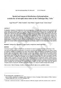
5. Results and Discussion 5.1. DT model Figure 5 shows the results of DT model, with nine terminal nodes. This means that it was not possible to define new rules to split these nodes and find more homogenous nodes. According to this figure, the time of crash, speed limit, pedestrian age, and POI are the primary splitters in this model. This implies that these variables are critical in classifying the severity of vehicle-pedestrian crashes in the Melbourne metropolitan area. Interestingly, the initial split at first node is based on the time of crash variable. This reveals that the most important influencing variable to classify the severity of vehicle-pedestrian crashes is the time of crash. Furthermore, Figure 5 shows that 25% of the pedestrian crashes occurred between 19:00 PM and 6:00 AM (night time). However, a considerable per-cent (about 60%) of these accidents were fatal or serious injury. This indicates that the risk of severe crashes occurring during this period is higher than other times. Part of the reason for the above result is provided by the next split node. For vehiclepedestrian crashes which occurred during the night, speed is the second splitter variable. According to Figure 5, pedestrians are more likely to be killed or harmed in a crash during night and on roads with a speed limit higher than 80 km/h. This figure reveals that pedestrian crashes during the night and on roads with a speed limit of more than 80 km/h are more likely to be fatal (19%) or injury crashes (62%). This is a significant result that shows that both time and speed limit are significant risk factors in vehicle-pedestrian crashes.

10


Figure

5: The Decision Tree for Pedestrian Crashes.

11


1 2 3 4 5 6 7 8 9 10 11 12 13 14

On the other hand, for vehicle-pedestrian crashes which occurred during the day, the pedestrian’s age is the most significant variable to classify the severity of the crash. Figure 5 shows that for day time crashes, the severity of traffic crash for ageing pedestrians (>65) is higher than all other age groups. Also, for this age group, POI is a significant classifier variable. This finding reveals that for day time crashes, aged pedestrians are more likely to be injured or killed (about 60%) and for this group of pedestrians, the type of POIs is an important factor. However, for other age groups, speed and POI are selected to classify the data for following branches. These results indicate that road safety strategies such as reducing travel speed close to POIs (e.g. government offices, playgrounds and health centres) can improve road safety and decrease the severity of vehicle-pedestrian crashes. Furthermore, Table 2 shows the relative importance of different variables influencing vehiclepedestrian crashes in Melbourne metropolitan area. According to this table, pedestrian age, POI, time of crash, and speed are the four most significant variables. These variables have the greatest (75%-100%) impact on vehicle-pedestrian crash severity.

15 16 17 18 19

In summary, the DT model (Figure 5 and Table 2) confirms that temporal and spatial variables (time and POI) have a significant impact on vehicle-pedestrian crash severity. Therefore, it is important to consider temporal and spatial characteristics of pedestrian crashes in crash or injury severity analysis to improve our understanding of the road safety issues for this group of road users.

20

5.2. Spatial autocorrelation

21 22 23 24 25 26 27 28 29

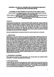
Spatial autocorrelation is applied to show the dependency between the location and time of vehicle-pedestrian crashes. Moran’s I is calculated multiple times with different increasing distance thresholds. Figure 6 shows the results of Moran’s I for vehicle-pedestrian crashes during day and night. This figure indicates that there is a positive correlation between time and location of vehicle-pedestrian crashes for day and night crashes. In addition, according to Figure 6, Moran’s I for 100m and 150m distance thresholds have the highest magnitude for day and night crashes, respectively. In addition, Figure 6 shows that the maximum Zscore is 3.0 for day and 5.6 for night crashes. In addition, Moran’s I relative to maximum Zscore is 0.03 for vehicle-pedestrian crashes during the day and 0.06 for night accidents.

30

Figure 6: Z-score and Moran's I for (a) day and (b) night crashes.

31 32 33 34 35 36 37

These results for Z-score and Moran’s I illustrate that the dependency between crash time and location is more significant during the night (19:00 PM to 6:00 AM) than during the day. Furthermore, the Z-scores of 5.6 and 3.0 (ρ=0.00) for 150m and 100m radii indicate there is less than 1% chance that this clustered pattern could be the result of a random choice. These findings reveal that there is a significant relationship between the time and location of vehicle-pedestrian crashes. This relationship is more significant for crashes during the night.

38

5.3. Temporal analysis

39 40 41

In this research, spider plots are applied to analyse the temporal distribution of vehiclepedestrian crashes in the Melbourne metropolitan area. Figure 7 illustrates how the vehiclepedestrian crashes are distributed during different times of the day. This figure shows two

12


1 2 3 4 5 6

peaks at 15:00 PM and 8:00 AM and a slight peak at 17:00 PM. According to Victoria traffic monitor reports on 2013, there are two traffic peak period times between 7:30 AM to 9:00 AM and 4:30PM to 6:00 PM and one off peak period between 10:00 AM to 15:00 PM in the road network of Melbourne metropolitan area (Victoria 2014). It should be noted that according to Figure 7, most pedestrian crashes occur during the off-peak traffic time (10:00 AM to 15:00 PM).

7

Figure 7: Temporal distribution of pedestrian crashes.

8 9 10 11 12 13 14 15 16 17

Interactive DT models provide the opportunity to classify the dataset according to a particular variable (e.g. speed, age, POI). Applying interactive DT for off-peak crashes shows that age of pedestrians is a significant variable to classify these crashes (Figure 8). This figure shows that for pedestrians older than 65 years of age who are involved in crashes, POI is an important variable. More than 70% of crashes for this category occurred around other POI, including aged cares, churches and offices. For the other age groups, speed and POI are the most important variables to classify crashes during off-peak traffic. For these pedestrians, education centres, general offices and local government offices are the important POIs.

18

Figure 8: Interactive DT for crashes occurring from 10:00 AM to 15:00 PM.

19 13


1 2 3 4 5 6 7 8 9 10 11 12 13 14

Figure 9 illustrates the temporal patterns of vehicle-pedestrian crashes for different age groups. According to this figure, different age groups have different crash patterns during the day and night. School age groups (0-18 years old) have two peaks at 8:00 AM and 15:00 PM when they go to school and return home. However, for pedestrians between 19 and 35 years of age, this figure shows that most of the crashes occur after 17:00 PM, when most of them finished work. For pedestrians older than 65 years of age, 9:00 AM to 12:00 PM and 15:00 PM are high risk times. These findings reveal that off-peak traffic time is more important in vehicle-pedestrian crashes. Furthermore, these results indicate that different safety strategies must be considered for different age groups. For pedestrians at school age, improving safety around schools and increasing the traffic safety awareness of children (e.g. safety education, walking to or from schools under supervision, etc.) might be helpful in decreasing the risk of crash for this age group. However, for pedestrians between 19 and 35 years of age, safety strategies targeted at evening attractions, such as restaurant and bars, must be considered.

15

Figure 9: Temporal pattern of pedestrian crashes for different age groups.

16 17 18 19 20 21 22 23 24 25 26 27 28 29 30

Figure 10 illustrates the distribution of vehicle-pedestrian crashes over different times of the day and days of the week. It is clear that the patterns of vehicle-pedestrian crashes are different during the 24 hours on weekdays and weekends. During the weekdays, most crashes occurred between 8:00 AM to 18:00 PM, while many weekend crashes occurred late at night and early in the morning (23:00 PM to 1:00 AM). In addition, pedestrian crash patterns at different times on Friday are different from other weekdays. Figure 10 shows that there are more crashes between 20:00 PM and 23:00 PM on Friday night. Interestingly, there are different crash peaks for Saturdays and Sundays between 23:00 PM to 1:00 AM. One possible explanation for these results is that more people go out on Friday nights than Sunday nights. These results show that it is important to consider targeted pedestrian safety strategies for these periods of time, such as increasing the visibility of pedestrians at night by improving street lighting or encouraging pedestrians to carry a flashlight or wear retroreflective clothing). Some strategies to manage alcohol consumption and drink walking should be considered, especially on Friday and Saturday nights.

31

14


1

Figure 10: Temporal distribution of vehicle-pedestrian crashes.

2 3 4 5 6 7

Table 3 shows the distribution of crashes for each severity level across different days of the week. According to this table, vehicle-pedestrian crashes occur most frequently on Friday (17.1%), followed by Thursday (16.1%). Moreover, Thursdays with 18.4% and Saturdays with 16.9% have the highest percentages of fatal crashes. Also, Table 3 shows that most of the serious injury crashes occur on Thursdays (15.6%) and Fridays (17.4%).

8

Table 2: Relative importance variables. Variable Name

Importance

Number of Rules in CV Trees

Relative Importance

Pedestrian Age

1

81

1

POI

0.96

159

0.93

Hour

0.88

48

0.92

Speed

0.75

58

0.80

Month

0.58

49

0.43

Node

0.51

31

0.36

Driver Age

0.47

11

0.18

Day

0.38

32

0.29

Pedestrian Gender

0.25

16

0.27

Driver Gender

0.20

1

0.05

9 10 11 12 13 14 15 16 17

Figure 11 shows the distribution of crashes with different severity levels for each day of the week. In addition, Table 3 and Figure 11 reveal that, only about 22% of pedestrian crashes occur during the weekend. However, more than 50% of pedestrian crashes which occur on Saturdays and Sundays are serious or fatal injury crashes. Figure 11 shows that the percentage of fatal and sever injury crashes reaches the highest value on Saturday and Sunday (54% and 52%, respectively), followed by Friday (50%). Traffic is usually lower on weekends and drivers tend to drive faster than on other days. This reason and the higher chance of pedestrian or driver intoxication are factors contributing to the higher severity of

15


1 2 3

vehicle-pedestrian crashes at weekends. Therefore, it is essential to consider appropriate countermeasure, such as increasing drink-driving and drink-walking enforcement, for improving pedestrian safety during these days.

4

Table 3: Distribution of crashes for each severity level across different days. Day

Sunday

Monday

Tuesday

Wednesday

Thursday

Friday

Saturday

Fatal

9.7%

13.8%

12.5%

13.1%

18.4%

15.6%

16.9%

Serious injury

10.4%

13.6%

14.3%

15.3%

15.6%

17.4%

13.2%

Other injury

9.2%

14.2%

17.2%

14.9%

16.4%

17.0%

11.2%

Total

9.8%

13.9%

15.7%

15.0%

16.1%

17.1%

12.3%

Severity

5

Figure 11: Distribution of crash severity for different days.

6 7

5.4. Spatial analysis

8 9 10 11 12 13

Figure 12 illustrates the vehicle-pedestrian crash distribution throughout the Melbourne metropolitan area over different time periods. These figures show that vehicle-pedestrian crash patterns are different during day and night. According to these figures, vehiclepedestrian crashes are not significant in some suburbs such as Mornington, Keysborough and Ringwood during the day. However, the numbers of crashes are considerable for these suburbs during the night.

14 15 16 17 18 19 20 21 22

KDE is applied to analyse the spatial distribution of vehicle-pedestrian crashes and identify locations with high risk of vehicle-pedestrian crashes in different periods of time. Figure 13 shows the spatial distribution of pedestrian crashes between (a) 7:00 AM to 9:00 AM, (b) 10:00 AM to 15:00 PM, (c) 16:00 PM to 18:00 PM, (d) 19:00 PM to 23:00 PM, and (e) 00:00 to 6:00 AM in magnified map of the Melbourne metropolitan area. These figures show that the distribution of vehicle-pedestrian crashes in Melbourne varies according to the time of day. In general, vehicle-pedestrian crashes are highly concentrated in the Melbourne central suburbs. However, these tend to relatively more disperse during the day but comparatively more concentrated in few areas around south-east suburbs during the night.

23 24 25 26 27 28 16


1

Figure 12: Distribution of vehicle-pedestrian crashes during (a) night and (b) day.

2 3 4 5 6 7 8 9 10 11

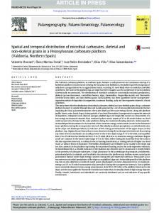
As shown by spider graph in Figure 13(f), vehicle-pedestrian crashes are most frequently reported to occur between 8-9 AM and 15-18 PM when people who work in Central Business District (CBD) commute to work or leave their work places. The existence of many offices, shopping centres and two Universities in Melbourne CBD provide many origins and destinations for pedestrian trips. These POIs increase the number of trips and consequently the risks of vehicle-pedestrian crashes in these areas (see Figures 13a, 13b, and 13c). However, Figures 13d and 13e reveal that between 19:00 and 23:00 PM and 00:00 and 6:00 AM, there are several high risk areas for pedestrians, including Melbourne CBD, St. Kilda, Windsor and Prahran.

12 13 14 15 16 17 18 19 20 21 22 23

As mentioned before, alcohol consumption might be one of the important factors contributing vehicle-pedestrian crashes in these periods of time. Thus, this study uses Google map to find the distribution of bars, clubs and restaurants in the Melbourne metropolitan area. As Figure 14a presents, there are many bars and restaurants in CBD. In addition, St. Kilda beach and bars around this beach are the destination of many pedestrians during weekend evenings. Furthermore, as Figures 12d, 12e, 14b and 14c show, Chapel Street is another area with high risk of vehicle-pedestrian crashes during the night. Figure 14a shows that there are many bars, clubs and restaurant in this street as well. Interestingly, comparing these figures show that most areas with high density of vehicle-pedestrian crashes (orange and red shades in KDE results) are also areas with a high number of bars and restaurants. Therefore, intoxication may be the main reason for vehicle-pedestrian crashes in these areas.

17


Figure 13: Spatial pattern of vehicle-pedestrian crash in different time periods.

18

Australasian Transport Research Forum 2016 Proceedings 16 – 18 November 2016, Melbourne, Australia Publication website: http://www.atrf.info Figure 14: Distributions of bars and restaurants (a) and high crash areas (b) 19-23 PM (c) 0-6 AM.

19


6. Conclusions and future research directions The main aim of this study was to examine the spatial and temporal distribution of vehiclepedestrian crashes in Melbourne metropolitan area and to identify areas and times with high crash risk for these vulnerable road users. DT model was applied with 10 explanatory variables to explore their influence on vehicle-pedestrian crash severity. This model revealed that the time of crash is the most significant variable influencing the classification of vehiclepedestrian crash severity. It also showed that speed limit and POIs are other important variables for vehicle-pedestrian crash severity. In addition, the analyses of spatial autocorrelation showed that there is a significant dependency between time and location of vehicle-pedestrian crashes. This dependency between time and location of crashes is greater during the night. Therefore, spider plots and KDE were applied to explore the temporal and spatial distribution of vehicle-pedestrian crashes in the Melbourne metropolitan area. Temporal analysis indicated that most crashes occur between 8:00 AM to 18:00 PM on weekdays. However, the frequency and severity of pedestrian crashes are higher during night time on weekends. About 22% of vehiclepedestrian crashes occur on weekends (Saturdays and Sundays) and half of them are fatal or serious injury crashes. Moreover, KDE analysis identified the areas with high risk of vehicle-pedestrian crashes in Melbourne metropolitan area for different time periods. Results of KDE identified that the risk of vehicle-pedestrian crashes is significant around the Melbourne CBD during the day. However, there are different vehicle-pedestrian crash patterns during the night. Spatiotemporal analysis revealed that St. Kilda beach and Chapel Street are the two areas with a high risk of vehicle-pedestrian crashes during the night and on weekends. The existence of bars, clubs and restaurants around these areas might increase pedestrian and vehicular traffic in these areas. Also, alcohol consumption by drivers or pedestrians might be the other important reason for vehicle-pedestrian crashes at nights during weekends in these areas. Evidence based road safety strategies, such as drinking-driving and drink-walking enforcement, targeting these times and locations would be required to improve pedestrian safety.

References Aguero-Valverde, J & Jovanis, PP 2006, 'Spatial analysis of fatal and injury crashes in Pennsylvania', Accident Analysis & Prevention, vol. 38, no. 3, pp. 618-25. Andrey, J & Yagar, S 1993, 'A temporal analysis of rain-related crash risk', Accident Analysis & Prevention, vol. 25, no. 4, pp. 465-72. Bíl, M, Andrášik, R & Janoška, Z 2013, 'Identification of hazardous road locations of traffic accidents by means of kernel density estimation and cluster significance evaluation', Accident Analysis & Prevention, vol. 55, no. 0, pp. 265-73. Black, WR 1991, 'Highway accidents: a spatial and temporal analysis', Transportation Research Record, no. 1318. Blazquez, CA & Celis, MS 2013, 'A spatial and temporal analysis of child pedestrian crashes in Santiago, Chile', Accident Analysis & Prevention, vol. 50, no. 0, pp. 304-11. Blockeel, H & Struyf, J 2002, 'Efficient algorithms for decision tree cross-validation', Journal of Machine Learning Research, vol. 3, no. Dec, pp. 621-50. Chainey, S, Reid, S & Stuart, N 2002, When is a hotspot a hotspot? A procedure for creating statistically robust hotspot maps of crime, Taylor & Francis, London, England. 20


Chang, L-Y & Wang, H-W 2006, 'Analysis of traffic injury severity: An application of non-parametric classification tree techniques', Accident Analysis & Prevention, vol. 38, no. 5, pp. 1019-27. Depren, O, Topallar, M, Anarim, E & Ciliz, MK 2005, 'An intelligent intrusion detection system (IDS) for anomaly and misuse detection in computer networks', Expert Systems with Applications, vol. 29, no. 4, pp. 713-22. Elvik, R, Vaa, T, Erke, A & Sorensen, M 2009, The handbook of road safety measures, Emerald Group Publishing. Flahaut, B, Mouchart, M, San Martin, E & Thomas, I 2003, 'The local spatial autocorrelation and the kernel method for identifying black zones. A comparative approach', Accid Anal Prev, vol. 35, no. 6, pp. 991-1004. Friedl, MA & Brodley, CE 1997, 'Decision tree classification of land cover from remotely sensed data', Remote sensing of environment, vol. 61, no. 3, pp. 399-409. Kashani, AT & Mohaymany, AS 2011, 'Analysis of the traffic injury severity on twolane, two-way rural roads based on classification tree models', Safety Science, vol. 49, no. 10, pp. 1314-20. Kohavi, R 1995, 'The power of decision tables', in N Lavrac & S Wrobel (eds), Machine Learning: ECML-95: 8th European Conference on Machine Learning Heraclion, Crete, Greece, April 25–27, 1995 Proceedings, Springer Berlin Heidelberg, Berlin, Heidelberg, pp. 174-89. Kuter, S, Usul, N & Kuter, N 2011, 'Bandwidth determination for kernel density analysis of wildfire events at forest sub-district scale', Ecological Modelling, vol. 222, no. 17, pp. 3033-40. Levine, N & CrimeStat, I 2002, 'A spatial statistics program for the analysis of crime incident locations', Ned Levine and Associates, Houston, TX, and the National Institute of Justice, Washington, DC. Levine, N, Kim, KE & Nitz, LH 1995, 'Spatial analysis of Honolulu motor vehicle crashes: I. Spatial patterns', Accident Analysis & Prevention, vol. 27, no. 5, pp. 663-74. Li, L, Zhu, L & Sui, DZ 2007, 'A GIS-based Bayesian approach for analyzing spatial– temporal patterns of intra-city motor vehicle crashes', Journal of Transport Geography, vol. 15, no. 4, pp. 274-85. Loo, BPY, Shenjun, Y & Jianping, W 2011, 'Spatial point analysis of road crashes in Shanghai: A GIS-based network kernel density method', paper presented to Geoinformatics, 2011 19th International Conference on, 24-26 June 2011. Miranda-Moreno, LF, Morency, P & El-Geneidy, AM 2011, 'The link between built environment, pedestrian activity and pedestrian–vehicle collision occurrence at signalized intersections', Accident Analysis & Prevention, vol. 43, no. 5, pp. 1624-34. Mitchell, A 2005, The ESRI guide to GIS analysis, Volume 2: Spatial Measurements and Statistics. Redlands, CA: Esri Press. O'Sullivan, D & Unwin, DJ 2003, Geographic information analysis, John Wiley & Sons. Pink, B 2010, 2009-2010 Year Book Australia, CANBERRA. Plug, C, Xia, JC & Caulfield, C 2011, 'Spatial and temporal visualisation techniques for crash analysis', Accident Analysis & Prevention, vol. 43, no. 6, pp. 193746. Pulugurtha, SS, Krishnakumar, VK & Nambisan, SS 2007, 'New methods to identify and rank high pedestrian crash zones: An illustration', Accident Analysis & Prevention, vol. 39, no. 4, pp. 800-11. 21


Sandhu, HAS, Singh, G, Sisodia, MS & Chauhan, R 2016, 'Identification of Black Spots on Highway with Kernel Density Estimation Method', Journal of the Indian Society of Remote Sensing, pp. 1-8. Schabenberger, O & Gotway, CA 2004, Statistical methods for spatial data analysis, CRC Press. Schneider, RJ, Ryznar, RM & Khattak, AJ 2004, 'An accident waiting to happen: a spatial approach to proactive pedestrian planning', Accident Analysis & Prevention, vol. 36, no. 2, pp. 193-211. Shen, C, Li, C & Si, Y 2016, 'Spatio-temporal autocorrelation measures for nonstationary series: A new temporally detrended spatio-temporal Moran's index', Physics Letters A, vol. 380, no. 1–2, pp. 106-16. Siddiqui, C, Abdel-Aty, M & Choi, K 2012, 'Macroscopic spatial analysis of pedestrian and bicycle crashes', Accident Analysis & Prevention, vol. 45, pp. 382-91. Silverman, BW 1986, Density estimation for statistics and data analysis, vol. 26, CRC press. Thakali, L, Kwon, TJ & Fu, L 2015, 'Identification of crash hotspots using kernel density estimation and kriging methods: a comparison', Journal of Modern Transportation, vol. 23, no. 2, pp. 93-106. Truong, LT & Somenahalli, SV 2011, 'Using GIS to identify pedestrian-vehicle crash hot spots and unsafe bus stops', Journal of Public Transportation, vol. 14, no. 1, pp. 99-114. Vicroads 2015, Toward Zero, Roads Corporation of Victoria. ---- 2016, interactive crash statistics application CrashStats 2010-2016, 2016 edn, Roads Corporation of Victoria, Victoria, Melbourne, 2016, . Victoria, PT 2014, Yarra Trams network map, Public transport victoria . WHO 2013, Pedestrian Safety, A road safety manual for decision-makers and practitioners, World Health Organization. Xie, Z & Yan, J 2008, 'Kernel Density Estimation of traffic accidents in a network space', Computers, Environment and Urban Systems, vol. 32, no. 5, pp. 396406. ---- 2013, 'Detecting traffic accident clusters with network kernel density estimation and local spatial statistics: an integrated approach', Journal of Transport Geography, vol. 31, no. 0, pp. 64-71.

22