MARINE ECOLOGY PROGRESS SERIES Mar Ecol Prog Ser
Vol. 478: 185–195, 2013 doi: 10.3354/meps10166
Published March 25
Spatial and temporal predictions of inter-decadal trends in Indian Ocean whale sharks Ana M. M. Sequeira1,*, Camille Mellin1, 2, Steven Delean1, Mark G. Meekan3, Corey J. A. Bradshaw1, 4 1
The Environment Institute and School of Earth and Environmental Sciences, The University of Adelaide, South Australia 5005, Australia 2 Australian Institute of Marine Science, PMB No. 3, Townsville MC, Townsville, Queensland 4810, Australia 3 Australian Institute of Marine Science, UWA Oceans Institute (MO96), 35 Stirling Hwy, Crawley, Western Australia 6009, Australia 4 South Australian Research and Development Institute, PO Box 120, Henley Beach, South Australia 5022, Australia
ABSTRACT: The processes driving temporal distribution and abundance patterns of whale sharks Rhincodon typus remain largely unexplained. We present an analysis of whale shark occurrence in the western Indian Ocean, incorporating both spatial and temporal elements. We tested the hypothesis that the average sighting probability of sharks has not changed over nearly 2 decades, and evaluated whether variance in sightings can be partially explained by climate signals. We used a 17 yr dataset (1991 to 2007, autumn only) of whale shark observations recorded in the logbooks of tuna purse-seiners. We randomly generated pseudo-absences and applied sequential generalized linear mixed-effects models within a multi-model information-theoretic framework, accounting for sampling effort and random annual variation, to evaluate the relative importance of temporal and climatic predictors to sighting probability. After accounting for seasonal patterns in distribution, we found evidence that sighting probability increased slightly in the first half of the sampling interval (1991−2000) and decreased thereafter (2000−2007). The model including a spatial predictor of occurrence, fishing effort, time2 and a random spatial effect explained ~60% of the deviance in sighting probability. After including climatic predictors, we found that sighting probability increased slightly with rising temperature in the central Pacific Ocean and reduced temperatures in the Indian Ocean. The declining phase of the peak, concurrent with recent accounts of declines in population size at near-shore aggregations and with the most pronounced global warming, deserves continued investigation. Teasing apart the legacy effects of past exploitation and those arising from on-going climate changes will be a major challenge for the successful longterm management of the species. KEY WORDS: Temporal trends · Rhincodon typus · Tuna purse-seine fisheries · Generalized linear mixed-effects models · Spatial distribution · Satellite data Resale or republication not permitted without written consent of the publisher
Understanding the mechanisms driving observed patterns in species occurrences in space and time is a key and challenging objective in ecology (Pimm et al. 1995, Gotelli et al. 2010). While global declines in
exploited marine fish species are well documented (Jackson et al. 2001, Roberts 2002, Pauly et al. 2005), the evidence for large shifts in distribution and abundance of much of the world’s biota arising from a warming climate is also mounting (e.g. Walther et al. 2002, Parmesan 2006, Traill et al. 2010). However,
*Email:
[email protected]
© Inter-Research 2013 · www.int-res.com
INTRODUCTION
186
Mar Ecol Prog Ser 478: 185–195, 2013
considerably less evidence is available for climate change-induced shifts in the marine environment (but see Hoegh-Guldberg & Bruno 2010, Last et al. 2011, Sumaila et al. 2011, Wernberg et al. 2011), principally due to the physical and economic constraints of collecting long-term datasets in the marine realm (Richardson & Poloczanska 2008). These problems are exacerbated for elusive migratory marine species because the low probability of detection can become an important issue in quantifying trends (Gotelli et al. 2010) and in disentangling spatial and temporal patterns. The whale shark Rhincodon typus (Smith 1828) is a highly migratory species (Sequeira et al. 2013) found in warm and temperate waters around the globe (Last & Stevens 1994). Aggregating seasonally near the shore at specific coastal locations (e.g. Rowat 2007), it is an important species both for fishing (Pravin 2000) and ecotourism industries (Rowat & Engelhardt 2007). Due to the species’ poorly quantified population size, demography and behaviour, as well as evidence for regional declines (Bradshaw et al. 2007, 2008), the legal targeted commercial fisheries have been banned (Theberge & Dearden 2006, Bradshaw et al. 2008), and whale sharks are now classified as Vulnerable in the IUCN Red List (www. iucnredlist.org). In contrast, whale shark ecotourism is growing worldwide (e.g. Rowat & Engelhardt 2007, Pierce et al. 2010, Hsu et al. 2012), but is highly dependent on the expectation that the sharks will return to the same locations every year. Whale shark sighting rates within these locations are highly variable, even within the same months (e.g. de la Parra Venegas et al. 2011). Such variation in local occurrence has been associated with fluctuations in climatic signals such as El Niño events and the Southern Oscillation index (Wilson et al. 2001, Sleeman et al. 2010a). Several attempts have been made to quantify trends in whale shark population size and abundance (Meekan et al. 2006, Rowat et al. 2009a), although these studies have been based mostly on data from near-shore aggregations composed largely of juvenile males (Meekan et al. 2006). Due to the transitory nature of whale shark occurrence, some have suggested that regional approaches should instead be used to quantify broader-scale patterns, spatial patterns and temporal trends (Rowat et al. 2009b). However, expanding a study site from 1 aggregation to an entire region (which might include multiple aggregation sites) inevitably results in adding spatial complexity to the process. Partitioning variance across spatial and temporal gradients to detect patterns in species occurrence is
not usually straightforward, but can be addressed statistically through the use of random-effects models (see Ogle 2009, Qian et al. 2010). These multilevel, mixed-effects or hierarchical models have been used extensively to understand temporal trends in species assemblages (Gotelli et al. 2010), community structure and patterns in the marine environment (e.g. MacNeil et al. 2009, Mellin et al. 2010), abundance and biomass of species (Ruiz & Laplanche 2010) and biological responses to different environmental conditions (Bedoya et al. 2011). Using a long-term (1991 to 2007) and wide-extent dataset of whale shark sightings in the Indian Ocean collected by the tuna purse-seine industry, we present an analysis incorporating both spatial and temporal elements to examine temporal trends of this species at the ocean-basin scale. Following previous work quantifying habitat suitability and seasonal variation in whale shark relative abundance in the Indian Ocean (Sequeira et al. 2012), our latest approach now partitions the complex spatial and temporal variation in whale shark occurrence patterns. Specifically, we tested the hypothesis that sighting probability remains constant over time, and quantified the influence of global climatic signals on temporal patterns of occurrence at a broad spatial scale.
METHODS We developed generalized linear mixed-effects models (GLMM) sequentially, with the first step assessing the evidence for a temporal trend in whale shark occurrence, and a second testing the hypothesis that sighting probability is correlated with variation in climatic indices. Below we detail the datasets used (presence/absence data and sampling effort) and the modelling steps (predictors and model development).
Whale shark dataset We used data recorded in logbooks from purseseine fishers registered under the Indian Ocean Tuna Commission (Pianet et al. 2009). These logbooks contain long-term (1991 to 2007) data on whale shark occurrences (hereafter referred to as ‘sightings’) derived from associated net-sets for tuna catch using whale sharks as fish aggregation devices. A total of 1185 sightings were recorded during the sampling period, including date and location at a 0.01° resolu-
Sequeira et al.: Inter-annual trends of whale shark occurrence
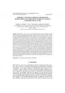
tion (i.e. latitude and longitude data were collected using the GCS WGS84 system and made available in units of decimal degrees to a precision of 0.01 degree). The dataset provided no indication of gender for the sighted sharks. Due to substantial fluctuation over time and higher numbers of sightings occurring mostly in autumn (Fig. 1a), we used data from this season to examine the inter-annual trends in autumn whale shark occurrence (Fig. S1 in the supplement at www.int-res.com/articles/suppl/m478 p185_supp.pdf shows spatial variation in occurrences). Seasonal patterns of whale shark occurrence in the same dataset were previously described by Sequeira et al. (2012).
187
presence recorded, we randomly generated 100 pseudo-absences (1:100 ratio) both (1) in space by randomly choosing non-presence grid cells over the western Indian Ocean (function srswor, i.e. simple random sampling without replacement, from the {Sampling} package in R), and (2) in time by randomly assigning to the selected point an autumn date within the 17 yr interval (function srswr, i.e. simple random sampling with replacement, from the {Sampling} package in R; R Development Core Team 2011). The high presence to pseudo-absence ratio (1:100), which inevitably results in low prevalence (0.01), allows a better representation of the ‘background’ available, which consisted of both spatial (each grid cell) and temporal (a specific date within the time period covered in the dataset) components.
Pseudo-absence generation Whale shark sightings were presence-only, so we generated pseudo-absences to produce the denominator of the logit function that allows for the binomial estimation in our GLMM detailed below. For each
Fisheries effort data
NINO4 index
IOD index
Autumn sightings
Whale shark sightings
Effort data (number of fishing days per month) were recorded with a resolution of 5° within the area covered by the fisheries (30° N to 30° S and 35° to 100° E; grey area in Fig. 2), a 150 ● giving a total of 1638 records (autumn Autumn only) and 13 674 fishing days with associated net-sets. The variables ‘effort’ and ‘number of sightings per ● 100 ● year’ are illustrated in Fig. 2. Because the eastern part of the Indian Ocean ● ● ● (east of the Maldives) was sampled ● 50 only in 1 year during autumn (1998; ● Fig. S1), we used only the western ● ●● ● ● ● area of the Indian Ocean (west of the ● ● ● ● ● ● ● ● ● ● ● ● ●● ● Maldives as depicted in Fig. 3) in our ● ● ● ● ● ● ●● ● ● ●● ● ●● ● ● ●● ●●●● ● ● ●●● ● ● ● ● ●● ● ●● ● ●●●● ● ● ●●● ●● ● ●● ● ● ● ● ● ●●● ● ●●●● ● ● ● ●● ●● ●● ● ●● ● ● ● ● ● ● ● ● ● ● ●● ● ● ●● ●● ●● ●● ● ● ●● ● ●● ● ● ●● ● ● ● ● ● ● ● ● ● ● ● ●● ● ● ● ● ● ● ●● ●● ● ● ● ● ● ● ● ●● ●●● ●● ●● ● ● ● ●● ● ● ● ● ●● ● ● ● ● ●● ● ●● ● ●● ● ●● 0 temporal analysis. 1991 1993 1995 1997 1999 2001 2003 2005 2007 Spatio-temporal variation in samYear pling effort can affect the ability to deb tect temporal trends in occurrence 200 30 200 (Phillips et al. 2009), so we developed WS 29.5 1.6 Index a series of generalized linear models 150 150 (GLM) with a Poisson error distribution 29 100 100 using time in years (Time) as a predic−0.1 28.5 tor for effort (in each of the 5° grid 50 50 28 squares sampled more than once dur−1.8 27.5 ing autumn), to test whether the spatial 0 0 1991 1995 1999 2003 2007 1991 1995 1999 2003 2007 patterns in sampling effort were Year Year evenly distributed throughout the 17 yr period. We compared the results Fig. 1. Rhincodon typus. (a) Total number of whale sharks sighted by tuna purse-seine fisheries per month and per year. Grey bar = autumn (April to of these models with a null (interceptJune from 1991 to 2007). (b) Total number of whale sharks (WS) sighted in only) model by calculating the eviautumn per year, overlaid with the values for the Indian Ocean Dipole (IOD dence ratio — a bias-corrected index of index; left) and sea surface temperature variation in Region 4 of the central the likelihood of one model over anPacific due to El Niño/La Niña events (NINO4 index; right). Black bars: median
Mar Ecol Prog Ser 478: 185–195, 2013
188
Fig. 2. Rhincodon typus. Example of variation in fishing effort (a,b) and number of whale sharks sighted (c,d). Only 2 yr of autumn (April to June from 1991 to 2007) data when effort was highest (1997, a,c) and lowest (2005, b,d) are shown. Light grey area = total area sampled by the tuna purse-seiners
other (wAICc (GLM Time) : wAICc (GLM null); see ‘Models’ below for definitions) — for each model. To control for inflation of Type I errors due to multiple testing across grid squares, we used the Holm correction through the Bioconductor {multtest} package (Pollard et al. 2005) in R (R Development Core Team 2011).
Model predictors This section describes the predictors used in each model step, detailing how we first accounted for temporal variation both in effort and sightings (Step 1), and then tested for correlations between observed trends and changes in climatic predictors (Step 2).
Step 1 Because temporal and spatial variation are seldom dissociated, we needed to include a term covering the variation in spatial probability of whale shark occurrence to test the hypothesis that the average probability of sightings remained constant over time within the large area under study. For this we used the results derived from Sequeira et al. (2012), where we fitted models of seasonal spatial distribution of whale sharks in the Indian Ocean. Here we re-fitted the whale shark distribution model for autumn (Sequeira et al. 2012), including some modifications to the likelihood estimation, pseudo-absence ratio
and covariate treatments (see the supplement at www.int-res.com/articles/supp/m478p185_supp.pdf for a detailed description of these changes). We then used logit-scale predictions of the likelihood of whale shark occurrence in autumn (spatial probability, ‘SpatialP’; Fig. S2 in the supplement) within each 9 km grid cell (resolution used by Sequeira et al. 2012) as an explanatory variable of whale shark occurrence in the temporal models developed herein. The inclusion of ‘SpatialP’ in the GLMM (see below) accounts for possible spatial autocorrelation. Temporal changes in effort can explain some of the inter-annual variation detected in sightings; therefore, we also added ‘effort’ as a predictor in our temporal models to account for its potential effect on the temporal patterns observed. Because the mean effort for autumn was already accounted for within the spatial predictor, we only included the temporal variation around the mean (i.e. the 0-centred inter-annual deviations around mean effort). We included both a fixed and a random effect for time (‘year ’ and ‘Time’, respectively) to account for inter-annual variability in presences, allowing the random structure to contain only information that could not have been modelled with fixed effects (following Zuur et al. 2009).
Step 2 To test the hypothesis that inter-annual variation in whale shark sightings was correlated with variation
Sequeira et al.: Inter-annual trends of whale shark occurrence
189
orology (www.bom.gov.au). To understand how the different indices are associated with each other and to assist interpretation of the model results, we investigated the correlation between the climatic predictors using the pairs.panels function in the package {psych} in R (R Development Core Team 2011) and their monotonic relationships using Spearman’s rank correlation (ρ). IOD is weakly collinear with both NINO4 and ONI (Pearson coefficients = 0.02 and −0.08, respectively), while the 2 latter predictors are highly correlated (Pearson coefficient = 0.89; Fig. S3). Spearman coefficients also showed collinearity only between NINO4 and ONI (ρ = 0.8).
Models
Fig. 3. Fishing effort analysis across the western Indian Ocean where the purse-seine fisheries operated in >1 yr (green line = limit of the western Indian Ocean area considered). Squares = 5° area for which fishing effort data were available, and colours = effort analysis results based on the GLM evidence ratios (ER) of the Akaike’s information criterion weight of ‘effort’ ~ ‘Time’ against the null model (i.e., wAICc GLM Time:wAICc GLM null). Values inside each square = estimates obtained for the coefficient of the ‘Time’ variable (when the null models were not ranked higher) after Holm correction
in indices of sea surface temperature (SST) and air pressure as reported previously in a near-shore aggregation (Wilson et al. 2001, Sleeman et al. 2010a), we considered variation in climatic indices in both the Indian and the Pacific Oceans. We tested 4 indices: (1) the Indian Ocean Dipole (IOD; Saji et al. 1999), (2) El Niño variation in the central Pacific Region 4, 160° E to 150° W, 5° S to 5° N (NINO4; Burgers & Stephenson 1999), (3) the Oceanic Niño Index (ONI), i.e. 3 mo moving averages of SST in the Niño 3.4 Region (170 to 120° W, 5° S to 5° N) and (4) the Southern Oscillation Index (SOI; Walker 1925). We collected the online climatic indices for the total period covered by the purse-seine fisheries from the Earth System Research Laboratory (US Department of Commerce, National Oceanic and Atmospheric Administration, www.esrl.noaa.gov/index. html), the Japanese Agency for Marine-Earth Science and Technology (www.jamstec.go.jp/frsgc/research/d1/ iod) and the Australian Government Bureau of Mete-
We applied GLMMs with a binomial error distribution and a logit link function to compare the predictive ability of different combinations of the predictors. The mixed-effects models we developed in each step included all possible combinations of the fixed and random effects (Step 1), and each of the 4 individual climatic predictors (Step 2). By including climatic variables 1 at a time, we concurrently tested whether replacing ‘Time’ by any of the climatic variables could explain away any trends observed in Step 1. In each step, we compared models based on Akaike’s information criterion corrected for small sample sizes (AICc; Burnham & Anderson 2004), which favours models with higher predictive capacity when sample sizes are large and tapering effects exist − as expected to occur in our spatio-temporal models. We assessed each model’s strength of evidence relative to the entire model set by calculating AICc model weights (wAICc ) and used the percentage of deviance explained (%De) to quantify each model’s goodnessof-fit. We retained the AICc top-ranked model from the first step and used it in the second step as a control model for the more complex combinations with climatic predictors. We developed all models in R version 2.11.1 (R Development Core Team 2011).
RESULTS Fisheries effort analysis The spatial analysis of effort (GLM models with Poisson distribution) per grid cell (5° resolution) demonstrated no evidence of temporal trend in effort in ~60% of the grid cells (Fig. 3). In the remaining cells, the evidence ratios of the models including
Mar Ecol Prog Ser 478: 185–195, 2013
190
‘Time’ were high (>> 150; Fig. 3), and effort generally increased over time (estimated coefficients ranging from 0.03 ± 0.008 to 0.23 ± 0.046 (mean ± SE); Fig. 3) with the exception of only 4 cells where effort decreased with time (coefficients ranging from −0.04 ± 0.005 to −0.12 ± 0.02; Fig. 3). Two of these 4 declining-effort cells corresponded to the area where most of the whale shark sightings occurred (compare Figs. 3 and S1).
Models Step 1 The GLMM with the highest information-theoretic support (wAICc = 0.45; Step 1) included the spatial predictor (i.e. spatial predictions of the probability of
whale shark occurrence in autumn on a logit scale — ‘SpatialP’; Fig. S2), the 0-centred effort (inter-annual variation around the autumn mean, i.e. the variation not accounted for by the spatial predictor), and a quadratic temporal trend with a random intercept term accounting for the among-year variance (Table 1). This model explained almost 60% of the deviance in whale shark sighting probability. We found evidence for a slight increase in the probability of whale shark sightings for the first half of the sampling period (1991−2000), and for a declining trend over the last half (2001−2007; Fig. 4). However, total wAICc was shared approximately evenly among the 2 top-ranked models (Table 1; only 1 of them including the ‘Time’ predictor), indicating that the temporal trend was only weak. Results for models not including the spatial term (‘SpatialP’) generally performed poorly relative to the other models in the set, with this
Table 1. Rhincodon typus. Generalized linear mixed-effects models relating probability of whale shark occurrence to: ‘SpatialP’, a spatial predictor derived from previous spatial distribution models (Sequeira et al. 2012), ‘effort’, ‘Time’ (fixed effect predictor for time in years) and a random effect for ‘year’ (Step 1); and global climatic predictors: IOD = Indian Ocean Dipole, SOI = Southern Oscillation Index, NINO4 = El Niño in the central Pacific-Region 4, and ONI = Oceanic Niño Index (Step 2). Shown for each model are the number of parameters (k), log-likelihood (LL), biased-corrected model evidence based on weights of Akaike’s information criterion corrected for small sample sizes (wAICc) and the percentage of deviance explained (%De). Best-performing models in each step are in bold. Models are ordered by decreasing wAICc. Values < 0.001 are not shown Model
k
LL
wAICc
%De
SpatialP + effort + Time + Time2 + (1| year) SpatialP + effort + (1| year) SpatialP + effort + Time + (1| year) SpatialP + effort SpatialP + effort + Time SpatialP + Time + Time2 + (1| year) SpatialP + (1| year) SpatialP + Time + (1| year) effort + Time + Time2 + (1| year) effort + (1| year) effort + Time + (1| year) SpatialP + Time SpatialP Time + Time2 + (1| year) 1 + (1| year) Time + (1| year) effort 1
7 5 6 5 6 6 4 5 6 4 5 5 4 5 3 4 4 3
−1956.08 −1958.29 −1958.03 −2531.80 −2531.72 −2707.72 −2710.93 −2710.87 −3201.41 −3203.59 −3202.95 −3313.77 −3317.50 −3995.69 −3998.67 −3998.23 −4025.96 −4544.22
0.454 0.370 0.176 < 0.001 < 0.001 < 0.001 < 0.001 < 0.001 < 0.001 < 0.001 < 0.001 < 0.001 < 0.001 < 0.001 < 0.001 < 0.001 < 0.001 < 0.001
57.0 56.9 56.9 44.3 44.3 40.4 40.3 40.4 29.6 29.5 29.5 27.1 27.0 12.1 12.0 12.0 11.4 0
SpatialP + effort + Time + Time2 + NINO4 + (1| year) SpatialP + effort + NINO4 + (1| year) SpatialP + effort + Time + Time2 + ONI + (1| year) SpatialP + effort + ONI + (1| year) SpatialP + effort + Time + Time2 + IOD + (1| year) SpatialP + effort + IOD + (1| year) SpatialP + effort + Time + Time2 + (1| year) SpatialP + effort + (1| year) SpatialP + effort + Time + Time2 + SOI + (1| year) SpatialP + effort + SOI + (1| year) 1
8 6 8 6 8 6 7 5 8 6 3
−1861.75 −1865.18 −1926.15 −1929.97 −1954.44 −1956.63 −1956.08 −1958.29 −1956.00 −1958.16 −4544.22
0.81 0.19 < 0.01 < 0.01 < 0.01 < 0.01 < 0.01 < 0.01 < 0.01 < 0.01 < 0.01
59.0 59.0 57.6 57.5 57.0 56.9 57.0 56.9 57.0 56.9 0
Step 1
Step 2
Sequeira et al.: Inter-annual trends of whale shark occurrence
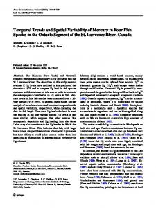
matic variables showed that an increase in NINO4 (reflecting higher SST in the central Pacific Ocean) had a positive effect on whale shark probability of occurrence in the western Indian Ocean (Fig. 5), and an increase in IOD (reflecting higher SST in the western part of the Indian Ocean) had a negative effect (Fig. S4).
Log odds of presence
−5 a −6 −7 −8
DISCUSSION
−9 0.005
Probability of presence
191
b
0.004 0.003 0.002 0.001
95 19 97 19 99 20 01 20 03 20 05 20 07
93
19
19
19
91
0.000
Year Fig. 4. Rhincodon typus. Partial effect of time (a) on the logodds scale showing the rate of change and (b) on the probability scale, showing the effect of time on the probability of whale shark presence. Dashed lines: 95% CI
predictor alone explaining 27% of the deviance (Table 1). A positive relationship with the 0-centred inter-annual deviations from mean (± SE) fishing effort (coefficient estimate = 1.63 ± 0.06) indicates that the number of sightings is higher when effort is higher than average and vice versa.
Step 2 Including the index of SST in the central Pacific (NINO4) in the highest-ranked model from Step 1 above resulted in the highest statistical support (wAICc = 0.81). However, the percentage of deviance explained (59%) was only slightly higher than the model excluding the climatic predictor (57%). All models that included a climatic predictor reflecting variation in sea surface temperature (NINO4, IOD, ONI) had higher support than those without climatic variables (from Step 1), while the model including SOI (relative to air pressure variation) performed poorly even when compared to models excluding climate signals (Table 1). The partial effects of the cli-
Access to a long-term dataset of whale shark sightings covering the western sector of an entire ocean basin provided a unique opportunity to analyse temporal trends and variation in whale shark occurrence at a scale more likely to encompass the range of this highly migratory species, and for a greater proportion of the population than in previous studies. Overall, our results highlighted a high inter-annual consistency in whale shark distribution patterns, with the spatial predictor (i.e. mean seasonal distribution) alone accounting for 27% of the deviance. We also found evidence for a modest peak in whale shark occurrences in the middle of the time series (~2000), which prevailed after accounting for changes in global climatic indices. To date, analogous temporal analyses of whale shark occurrence have only been done at the scale of single aggregations (~10s of km; Sleeman et al. 2010a) covering only a small part of this species’ range and only a small proportion of the population (mostly male juveniles, Meekan et al. 2006). Thus, our results are the first to estimate ocean-scale trends in occurrence that include several known aggregation sites for the species, and it is the first analysis to account simultaneously for spatial and temporal components, including effort, that can mask underlying trends in the probability of occurrence. The high percentage of deviance explained by the spatial predictor (27%) implies that distribution patterns are annually consistent (autumn only), with a higher probability of occurrence around the Mozambique Channel. This consistency might be due to permanent characteristics of the area, such as physical features enhancing upwelling, local productivity and tolerable sea surface temperatures (Sequeira et al. 2012). Modelling must ensure that variation in sampling effort does not confound results (Dennis et al. 1999). In our dataset, effort generally increased through time, although there was a decline in the Mozambique Channel (Fig. 3) where most sightings occurred during the 17 yr (cf. Fig. S1). By including the 0-centred inter-annual deviations from mean fishing
Mar Ecol Prog Ser 478: 185–195, 2013
a
−2
Log odds of presence (with NINO4)
Log odds of presence
192
−4 −6 −8 −10
−4
b
−6 −8 −10 −12
93 19 95 19 97 19 99 20 01 20 03 20 05 20 07
91
19
19
27
27
.3 5 .6 35 27 .9 2 28 .2 0 28 5 .4 9 28 .7 75 29 .0 6 29 .3 4 29 5 .6 3
−12
Year
c
d
Year
.6 3 27 5 .9 2 28 .2 0 28 5 .4 9 28 .7 7 29 5 .0 6 29 .3 45 29 .6 3
0.00 .3
97 19 99 20 01 20 03 20 05 20 07
95
19
19
19
19
93
0.000
0.02
27
0.005
0.04
27
0.010
0.06
5
Partial effect on presence
0.015
91
Probability of presence (with NINO4)
NINO4
NINO4
Fig. 5. Rhincodon typus. (a,d) Partial effect of NINO4 on the probability of whale shark presence. NINO4 is an index representing sea surface temperature variation in the central Pacific Region 4 (160° E to 150° W, 5° S to 5° N; Burgers & Stephenson 1999). (b,c) Partial effect of ‘Time’ after accounting for climatic contributions to whale shark probability of presence. Dashed lines: 95% CI
effort in our models (which represent temporal fluctuations from the mean within each grid cell; Sequeira et al. 2012), we accounted for the contribution of effort in the temporal probability of occurrence. Combining the spatial predictor just with effort, our models explained ~44% of the deviance (Table 1), demonstrating the importance of incorporating both spatial and sampling effort components in temporal models. We hypothesize that the weak non-linear temporal trend (Fig. 4) reflects variation in whale shark abundance rather than a change in behaviour that could lead to the lower sighting probability (e.g. a change in diving behaviour). Whale sharks spend most of the time at the surface (Sleeman et al. 2010b), a behaviour hypothesized to arise due to thermoregulatory requirements (Thums et al. 2012). We therefore forward 3 competing hypotheses to explain the non-linear trend observed: (1) a cyclic pattern in relative abundance (e.g. associated with inter-oceanic migratory behaviour), (2) a decline in population size (e.g. induced by fisheries; Sequeira et al. 2013) or (3) a distributional shift due to changing habitat characteristics (e.g. via climate change).
The complete trend observed, where the probability of occurrence first increases and then decreases, could represent an inter-decadal cycle (i.e. cycle over 15 yr) in whale shark occurrences, similar to strandings of other large marine species in the Southern Ocean (Evans et al. 2005) and fish catches in the same region (Jury et al. 2010). In the latter study, cycles were only just detectable even with annual catch records spanning 40 yr. Our dataset, covering < 20 yr, revealed weak evidence for a peak in whale shark occurrence that accords with the longer cycles found for fish catches (Jury et al. 2010). Within the Indian Ocean, the probability of whale shark occurrence during autumn is higher within the Mozambique Channel (Sequeira et al. 2012). Being a highly migratory species, the observed trend could be reflecting variation in whale shark abundance associated with migratory behaviour among ocean basins. This being the case, the decline observed would correspond only to a temporary decline in relative abundance, with the trend reversing at the onset of a new cycle. Focussing only on the declining segment of the identified peak, and assuming it reflects a real
Sequeira et al.: Inter-annual trends of whale shark occurrence
193
decline in population size (such as that associated Indian Ocean were higher than normal) and coinwith possible over-fishing), our results support previcided with a decrease in probability of occurrence in ous data (Bradshaw et al. 2008) and predictions the western Indian Ocean (Fig. S4). When IOD is pos(Bradshaw et al. 2007) from Ningaloo in Western itive, the thermocline deepens in the eastern Indian Australia that suggest a decline in population size. In Ocean, resulting in more intense upwelling and fact, the South-East Asian and Indian whale sharkgreater surface productivity in that area (Behera & targeted fisheries (Pravin 2000, Hsu et al. 2012) were Yamagata 2003). Saji et al. (1999) first described IOD banned due to the low numbers captured even with as independent of El Niño/Southern Oscillation, increasing effort — a signal that can indicate populaalthough others suggested possible associations betion decline. Despite the bans, targeted fisheries still tween them (reviewed by Maity et al. 2007). Underpresent a risk to whale sharks due to lack of enforcestanding how these coupled sea surface−atmosphere ment (Stewart & Wilson 2005), and there is evidence phenomena are related is not our aim, but the (weak) that illegal fishing is still occurring (White & support for Pacific and Indian Ocean indices suggest Cavanagh 2007, Riley et al. 2009). Such illegal fishsome possible effects of broad-scale oceanic climate eries could still be responsible for on-going declines, events influencing whale shark habitat use. although it is currently impossible to determine to Despite cycles in fish abundance in the western what extent this might still be occurring. The uninIndian Ocean being directly related to environmental tentional bycatch of whale sharks in other fisheries fluctuations, most of the variance in fish catch can be (e.g. purse seiners; Romanov 2002) also remains explained with estimates of local productivity (Jury unquantified. et al. 2010). Changes in climate are already affecting The decline segment is also concurrent with the the base of the principal food web, viz. phytoplankmost pronounced warming observed over the last ton (e.g. Edwards & Richardson 2004). This evidence, decade, such that a related hypothesis where latitucoupled with our demonstration of possible climatedinal shifts in distribution resulting from rising water influenced distribution of the world’s largest fish, temperatures (as suggested by Sequeira et al. 2012) demonstrates a need to predict how species will driven by global climate change could be influential. respond to future climate scenarios. As such, longEven though we found that autumn distribution patterm management of whale sharks requires both a terns were constant within the area considered, the better understanding of basic ecology and demogradecline could also arise if environmental conditions phy, and how these will be altered as the oceans allowed a shift in distribution to areas outside our warm. dataset’s spatial coverage, such as farther south, Acknowledgements. We thank the purse-seine vessel owncloser to the shores of South Africa or south of Madaers for access to log-book data and to the Indian Ocean Tuna gascar (Fig. 3). Our models’ estimates suggest that Commission and the Institut de Recherche pour le sighting probability increases with rising sea surface Développement (France), in particular A. Fonteneau, temperature in the central Pacific Ocean (i.e. high M. Herrera and R. Pianet for data extraction and D. Rowat for data availability and help with interpretation. Our study NINO4; Fig. 4) and reduced temperatures in the was funded by Fundação para a Ciência e Tecnologia and Indian Ocean (i.e. low IOD; Fig. S4). Despite IOD European Social Funds through A.M.M.S.’s PhD scholarship being a climatic index directly measured in the (SFRH/BD/47465/2008), The University of Adelaide, AusIndian Ocean, our models gave higher support for tralian Institute of Marine Science, Flying Sharks and the NINO4 as a predictor. However, there were some Portuguese Association for the Study and Conservation of Elasmobranchs. occasions where a few whale sharks were sighted despite high NINO4 values, that is, high sea surface temperatures in the central Pacific Ocean (Fig. 1). LITERATURE CITED This is particularly interesting for 1997, when not Bates D, Maechler M, Bolker B (2011) lme4: linear mixedonly the NINO4 index was high, but the sampling effects models using S4 classes. Available at www.cran.reffort was also maximal (Fig. 2). Our data covered project.org/web/packages/lme4/index.html mainly the western Indian Ocean, but there was a ➤ Bedoya D, Manolakos ES, Novotny V (2011) Characterizapeak in sightings at Ningaloo in 1997 (Wilson et al. tion of biological responses under different environmental conditions: a hierarchical modeling approach. Ecol 2001). The same occurred in 1992 (Wilson et al. 2001) Model 222:532−545 and 2002 (see Sleeman et al. 2010a), when NINO4 Behera SK, Yamagata T (2003) Influence of the Indian ➤ was high and few sharks were observed in the westOcean Dipole on the Southern Oscillation. J Meteorol ern Indian Ocean. In both 1997 and 2002, IOD was Soc Jpn 81:169−177 positive (0.04 to 0.88; i.e. temperatures in the western ➤ Bradshaw CJA, Mollet HF, Meekan MG (2007) Inferring
194
➤
➤ ➤
➤
➤ ➤
➤
➤
➤ ➤
➤
➤
➤
➤
➤
Mar Ecol Prog Ser 478: 185–195, 2013
population trends for the world’s largest fish from mark− recapture estimates of survival. J Anim Ecol 76:480−489 Bradshaw CJA, Fitzpatrick BM, Steinberg CC, Brook BW, Meekan MG (2008) Decline in whale shark size and abundance at Ningaloo Reef over the past decade: the world’s largest fish is getting smaller. Biol Conserv 141: 1894−1905 Burgers G, Stephenson DB (1999) The ‘normality’ of El Niño. Geophys Res Lett 26:1027−1030 Burnham KP, Anderson DR (2004) Multimodel inference: understanding AIC and BIC in model selection. Sociol Methods Res 33:261−304 de la Parra Venegas R, Hueter R, González Cano J, Tyminski J and others (2011) An unprecedented aggregation of whale sharks, Rhincodon typus, in Mexican coastal waters of the Caribbean Sea. PLoS ONE 6:e18994 doi: 10.11371/journal.pone.0018994 Dennis RLH, Sparks TH, Hardy PB (1999) Bias in butterfly distribution maps: the effects of sampling effort. J Insect Conserv 3:33−42 Edwards M, Richardson AJ (2004) Impact of climate change on marine pelagic phenology and trophic mismatch. Nature 430:881−884 Evans K, Thresher R, Warneke RM, Bradshaw CJA, Pook M, Thiele D, Hindell MA (2005) Periodic variability in cetacean strandings: links to large-scale climate events. Biol Lett 1:147−150 Gotelli NJ, Dorazio RM, Ellison AM, Grossman GD (2010) Detecting temporal trends in species assemblages with bootstrapping procedures and hierarchical models. Philos Trans R Soc Lond B Biol Sci 365:3621−3631 Hoegh-Guldberg O, Bruno JF (2010) The impact of climate change on the world’s marine ecosystems. Science 328: 1523−1528 Hsu HH, Joung SJ, Liu KM (2012) Fisheries, management and conservation of the whale shark Rhincodon typus in Taiwan. J Fish Biol 80:1595−1607 Jackson JBC, Kirby MX, Berger WH, Bjorndal KA and others (2001) Historical overfishing and the recent collapse of coastal ecosystems. Science 293:629−637 Jury M, McClanahan T, Maina J (2010) West Indian Ocean variability and East African fish catch. Mar Environ Res 70:162−170 Last PR, Stevens JD (1994) Sharks and rays of Australia, 2nd edn. CSIRO Publishing, Collingwood Last PR, White WT, Gledhill DC, Hobday AJ, Brown R, Edgar GJ, Pecl G (2011) Long-term shifts in abundance and distribution of a temperate fish fauna: a response to climate change and fishing practices. Glob Ecol Biogeogr 20:58−72 MacNeil MA, Graham NAJ, Polunin NVC, Kulbicki M, Galzin R, Harmelon-Vivien M, Rushton SP (2009) Hierarchical drivers of reef-fish metacommunity structure. Ecology 90:252−264 Maity R, Kumar DN, Nanjundiah RS (2007) Review of hydroclimatic teleconnection between hydrologic variables and large-scale atmospheric circulation patterns with Indian perspective. ISH J Hydraul Eng 13:77−92 Meekan MG, Bradshaw CJA, Press M, McLean C, Richards A, Quasnichka S, Taylor JG (2006) Population size and structure of whale sharks Rhincodon typus at Ningaloo Reef, Western Australia. Mar Ecol Prog Ser 319: 275−285 Mellin C, Bradshaw CJA, Meekan MG, Caley MJ (2010) Environmental and spatial predictors of species richness
➤ ➤ ➤ ➤
➤
➤
➤ ➤ ➤
➤ ➤
➤ ➤
and abundance in coral reef fishes. Glob Ecol Biogeogr 19:212−222 Ogle K (2009) Hierarchical Bayesian statistics: merging experimental and modeling approaches in ecology. Ecol Appl 19:577−581 Parmesan C (2006) Ecological and evolutionary responses to recent climate change. Annu Rev Ecol Evol Syst 37: 637−669 Pauly D, Watson R, Alder J (2005) Global trends in world fisheries: impacts on marine ecosystems and food security. Philos Trans R Soc Lond B Biol Sci 360:5−12 Phillips SJ, Dudík M, Elith J, Graham CH, Lehmann A, Leathwick J, Ferrier S (2009) Sample selection bias and presence-only distribution models: implications for background and pseudo-absence data. Ecol Appl 19:181−197 Pianet R, Delgado de Molina A, Doriso J, Dewals P, Norström V, Ariz J (2009) Statistics of the main purse seine fleets fishing in the Indian Ocean (1981-2008). IOTC-2009-WPTT-22. Indian Ocean Tuna Commission, Tropical Tunas Working Party, Mombasa Pierce SJ, Méndez-Jiménez A, Collins K, Rosero-Caicedo R, Monadjem A (2010) Developing a code of conduct for whale shark interactions in Mozambique. Aquatic Conserv 20:782−788 Pimm SL, Russell GJ, Gittleman JL, Brooks TM (1995) The future of biodiversity. Science 269:347−350 Pollard KS, Dudoit S, van der Laan MJ (2005) Multiple testing procedures: R multtest package and applications to genomics. In: Gentleman R, Carey VC, Huber W, Irizarry RS, Dudoit S (eds) Bioinformatics and computational biology solutions using R and Bioconductor. Springer, New York, NY, p 249−273 Pravin P (2000) Whale shark in the Indian coast — need for conservation. Curr Sci 79:310−315 Qian SS, Cuffney TF, Alameddine I, McMahon G, Reckow KH (2010) On the application of multilevel modeling in environmental and ecological studies. Ecology 91: 355−361 R Development Core Team (2011) R: a language and environment for statistical computing. R Foundation for Statistical Computing, Vienna. Available at www.Rproject.org Richardson AJ, Poloczanska ES (2008) Under-resourced, under threat. Science 320:1294−1295 Riley MJ, Harman A, Rees RG (2009) Evidence of continued hunting of whale sharks Rhincodon typus in the Maldives. Environ Biol Fishes 86:371−374 Roberts CM (2002) Deep impact: the rising toll of fishing in the deep sea. Trends Ecol Evol 17:242−245 Romanov EV (2002) Bycatch in the tuna purse-seine fisheries of the western Indian Ocean. Fish Bull 100:90−105 Rowat D (2007) Occurrence of whale shark (Rhincodon typus) in the Indian Ocean: a case for regional conservation. Fish Res 84:96−101 Rowat D, Engelhardt U (2007) Seychelles: a case study of community involvement in the development of whale shark ecotourism and its socio-economic impact. Fish Res 84:109−113 Rowat D, Gore M, Meekan MG, Lawler IR, Bradshaw CJA (2009a) Aerial survey as a tool to estimate whale shark abundance trends. J Exp Mar Biol Ecol 368:1−8 Rowat D, Speed CW, Meekan MG, Gore MA, Bradshaw CJA (2009b) Population abundance and apparent survival of the vulnerable whale shark Rhincodon typus in the Seychelles aggregation. Oryx 43:591−598
Sequeira et al.: Inter-annual trends of whale shark occurrence
➤ Ruiz P, Laplanche C (2010) A hierarchical model to estimate
➤ ➤
➤
➤
➤ ➤ ➤
the abundance and biomass of salmonids by using removal sampling and biometric data from multiple locations. Can J Fish Aquat Sci 67:2032−2044 Saji NH, Goswami BN, Vinayachandran PN, Yamagata T (1999) A dipole mode in the tropical Indian Ocean. Nature 401:360−363 Sequeira A, Mellin C, Rowat D, Meekan MG, Bradshaw CJA (2012) Ocean-scale prediction of whale shark distribution. Divers Distrib 18:504−518 Sequeira A, Mellin C, Meekan MG, Sims DW, Bradshaw CJA (2013) Inferred global connectivity of whale shark populations. J Fish Biol 82:367–389 Sleeman JC, Meekan MG, Fitzpatrick BJ, Steinberg CR, Ancel R, Bradshaw CJA (2010a) Oceanographic and atmospheric phenomena influence the abundance of whale sharks at Ningaloo Reef, Western Australia. J Exp Mar Biol Ecol 382:77−81 Sleeman JC, Meekan MG, Wilson SG, Polovina JJ, Stevens JD, Boggs GS, Bradshaw CJA (2010b) To go or not to go with the flow: environmental influences on whale shark movement patterns. J Exp Mar Biol Ecol 390:84−98 Smith A (1828) Descriptions of new, or imperfectly known objects of the animal kingdom, found in South Africa. South Afr Commer Advertiser 145:2 Stewart BS, Wilson SG (2005) Threatened fishes of the world: Rhincodon typus (Smith 1828) (Rhincodontidae). Environ Biol Fishes 74:184−185 Sumaila UR, Cheung WWL, Lam VWY, Pauly D, Herrick S (2011) Climate change impacts on the biophysics and economics of world fisheries. Nat Clim Change 1:449−456 Theberge MM, Dearden P (2006) Detecting a decline in whale shark Rhincodon typus sightings in the Andaman Sea, Thailand, using ecotourist operator-collected data. Oryx 40:337−342 Editorial responsibility: Nicholas Tolimieri, Seattle, Washington, USA
➤
➤ ➤ ➤
➤ ➤
➤
195
Thums M, Meekan M, Stevens J, Wilson S, Polovina J (2012) Evidence for behavioural thermoregulation by the world’s largest fish. J R Soc Interface 10:20120477 doi: 10.1098/rsif.2012.0477 Traill LW, Lim MLM, Sodhi NS, Bradshaw CJA (2010) Mechanisms driving change: altered species interactions and ecosystem function through global warming. J Anim Ecol 79:937−947 Venables WN, Ripley BD (2002) Modern applied statistics with S, 4th edn, Vol 1. Springer, New York, NY Walker G (1925) Correlation in seasonal variations of weather — a further study of world weather. Mon Weather Rev 53:252−254 Walther GR, Post E, Convey P, Menzel A and others (2002) Ecological responses to recent climate change. Nature 416:389−395 Wernberg T, Russell BD, Thomsen MS, Gurgel CFD, Bradshaw CJA, Poloczanska ES, Connell SD (2011) Seaweed communities in retreat from ocean warming. Curr Biol 21:1828−1832 White WT, Cavanagh RD (2007) Whale shark landings in Indonesian artisanal shark and ray fisheries. Fish Res 84: 128−131 Wilson SG, Taylor JG, Pearce AF (2001) The seasonal aggregation of whale sharks at Ningaloo Reef, Western Australia: currents, migrations and the El Niño / Southern Oscillation. Environ Biol Fishes 61:1−11 Wilson SG, Polovina JJ, Stewart BS, Meekan MG (2006) Movements of whale sharks (Rhincodon typus) tagged at Ningaloo Reef, Western Australia. Mar Biol 148: 1157−1166 Zuur AF, Ieno EN, Walker N, Saveliev AA, Smith GM (2009) Mixed effects models and extensions in ecology with R, 1st edn. Springer Science+Business Media LCC, New York, NY Submitted: July 19, 2012; Accepted: November 7, 2012 Proofs received from author(s): February 21, 2013