Spatial and Temporal Variations of Land Surface ... - BioOne

Mountain Research and Development (MRD) An international, peer-reviewed open access journal published by the International Mountain Society (IMS) www.mrd-journal.org

MountainResearch Systems knowledge

Spatial and Temporal Variations of Land Surface Temperature Over the Tibetan Plateau Based on Harmonic Analysis Yongming Xu1*, Yan Shen2, and Ziyue Wu3 * Corresponding author: [email protected] 1 School of Remote Sensing, Nanjing University of Information Science & Technology, 219 Ningliu Road, Nanjing 210044, China 2 National Meteorological Information Center, 46 Zhongguancun South Street, Beijing 100081, China 3 Pukou Meteorological Bureau of Nanjing, 325 Jianshe Road, Nanjing 210044, China Open access article: please credit the authors and the full source.

study area, and the spatial distribution of seasonal oscillation is closely related to precipitation. However, the timing of the peak LST does not exhibit an obvious regular pattern. The LST characteristics of different land cover types were also studied. Bare land has the highest mean LST and exhibits remarkable seasonal fluctuation. Snow, ice, or both show the lowest mean temperature, and forest shows the weakest seasonality. Different land cover types also reflect different peak occurrences of the LST annual cycle, with grassland showing the lowest annual phase value. This paper provides detailed information on the LST variations on the Tibetan Plateau, with the cloud contamination removed. The HANTS algorithm is demonstrated to be effective for understanding spatiotemporal variations of remotely sensed LST, especially for regions over which dense clouds cause large gaps in the LST data.

Land surface temperature (LST) is an essential parameter in the physics of land surface processes. The spatiotemporal variations of LST on the Tibetan Plateau were studied using AQUA Moderate Resolution Imaging Spectroradiometer LST data. Considering the data gaps in remotely sensed LST products caused by cloud contamination, the harmonic analysis of time series (HANTS) algorithm was used to eliminate the influence of cloud cover and to describe the periodical signals of LST. Observed air temperature data from 79 weather stations were employed to evaluate the fitting performance of the HANTS algorithm. Results indicate that HANTS can effectively fit the LST time series and remove the influence of cloud cover. Based on the HANTS-derived mean term and annual harmonics, annual mean LST, seasonal fluctuation, and peak time of the LST annual cycle are discussed. The spatial distribution of annual mean LST generally exhibits consistency with altitude in the

Keywords: Land surface temperature (LST); spatiotemporal variations; harmonic analysis; Moderate Resolution Imaging Spectroradiometer (MODIS); Tibetan Plateau. Peer-reviewed: November 2012 Accepted: December 2012

distribution of meteorological stations. Satellite remote sensing provides a straightforward and consistent way to observe LST over large scales with more spatially detailed information. During the past decades, LST retrieval has become a hot topic in remote sensing studies. Some classical approaches, such as split-window algorithm, monowindow algorithm, and single-channel algorithm, have been developed and have achieved satisfactory accuracy (Price 1984; Becker and Li 1990; Wan and Li 1997; Qin et al 2001; Jimenez-Munoz and Sobrino 2003). Based on LST data derived from remote sensing, several studies have been conducted to study the spatial and temporal variations of LST. Manzo-Delgado et al (2004) analyzed LST changes in central Mexico in the dry seasons from 1996 to 2000 and the relationships between LST and forest fires. Julien et al (2006) studied LST dynamics over the European continent from 1982 to 1999 using Advanced Very High Resolution Radiometer data.

Introduction Land surface temperature (LST) is an essential parameter in the physics of land surface processes: it plays a key role in the energy and water transfers between the ground and the atmosphere (Jin et al 1997). LST is controlled by solar radiation and the land–atmosphere heat exchange (Manzo-Delgado et al 2004). Therefore, its spatial and temporal distributions reflect not only the variations of climate factors but also the land surface characteristics. An in-depth understanding of the spatial and temporal variations of LST is important to a range of research fields, including climate, vegetation, and hydrology. Traditional LST data are collected by meteorological observation and then interpolated to gridded data. However, in some areas, especially in remote areas, spatial interpolation cannot provide satisfactory results from point observations due to the sparse density and uneven

Mountain Research and Development

Vol 33 No 1 Feb 2013: 85–94

85

http://dx.doi.org/10.1659/MRD-JOURNAL-D-12-00090.1 ß 2013 by the authors

MountainResearch

(Qiu 2008), the Tibetan Plateau is the highest and largest plateau in the world, with an average elevation of more than 4000 m above sea level. As a result of the high altitude, the climate of the plateau is quite different from that of other regions at nearly the same latitudes. The mean annual air temperature varies between 22.8 and 11.9uC, depending on the topographic conditions. The annual precipitation decreases from more than 800 mm in the southeast to lower than 200 mm in the northwest, with most precipitation occurring from May to September. Influenced by the climate and altitude, land cover on the Tibetan Plateau also shows a clear geographic distribution, following the order of forest, grassland, and desert from the southeast to the northwest (Wang et al 2005).

Westermann et al (2011) analyzed the spatial and temporal variations of the surface temperatures of higharctic tundra in the summer and assessed the long-term impact of snow cover, soil moisture, and surface cover on surface temperature. Van De Kerchove et al (2011) assessed the spatiotemporal variability of LST in the Russian Altai Mountains and its relationship with physiographic variables. As the highest and largest highland in the world, the Tibetan Plateau plays an important role in regional and global climate through thermal forcing mechanisms (Yanai et al 1992). The plateau’s surface absorbs a large amount of incoming solar radiation energy and undergoes seasonal variations of surface heat fluxes (Ye and Gao 1979). The quantitative analysis of LST is important for understanding the land–atmosphere energy balance of the plateau and its effects on climate. In recent decades, many studies have been performed to analyze the temperature changes of the Tibetan Plateau using meteorological observation data (Lin and Zhao 1996; Liu and Chen 2000; Du 2001; Xu et al 2003; Li et al 2005; Duan et al 2006; Liu et al 2006, 2009; Ding and Zhang 2008; Wang et al 2008a; You et al 2008; Cuo et al 2012). Due to the sparse density and uneven distribution of meteorological stations on the plateau, the spatial pattern of temperature cannot be properly depicted. Some efforts have been devoted to analyzing LST variations by remote sensing (Jiang and Wang 2001; Ma et al 2003; Oku et al 2006; Salama et al 2012; Tseng et al 2011; Zhong et al 2011). Most of these studies used coarse resolution remotely sensed LST data, which cannot represent detailed spatial patterns. In addition, the incompleteness of the remotely sensed LST caused by cloud cover has not been considered in these studies. Considering the Tibetan Plateau’s unique topography and its thermal forcing mechanism on atmospheric circulation, a study of the LST variations in this region is essential for understanding the energy and water cycle; therefore, it has important scientific significance in regional and global climate research. The main objective of this paper is to analyze the spatiotemporal variations of LST on the Tibetan Plateau using harmonic analysis, which can effectively eliminate cloud contaminations and depict fundamental periodic variations. The 1-km resolution Moderate Resolution Imaging Spectroradiometer (MODIS) LST product from 2003 to 2010 was employed in this study.

Data set

The AQUA MODIS LST product (MYD11A2) spanning 2003 to 2010 was obtained from the Warehouse Inventory Search Tool (WIST 2011). MYD11A2 is an 8-day composite daytime and nighttime LST product with a 1-km spatial resolution that is derived from AQUA MODIS data. The LST product is first computed using the generalized splitwindow algorithm proposed by Wan and Dozier (1996) and then produced by averaging the LST values under clear-sky conditions over an 8-day period (Wan et al 2002) for the purpose of removing cloudy pixels. In this study, the daytime LST was employed with an overpass time of approximately 1:30 PM (local solar time). First, the MODIS daily LST product was computed using the generalized split-window algorithm (Wan and Dozier 1996): 1{e De T31 zT32 zA3 2 ) e e 2 1{e De T31 {T32 zB3 2 ) , z(B1 zB2 e e 2 e~(e31 ze32 )=2, De~e31 {e32 , Ts ~Cz(A1 zA2

where Ts is LST; T31 and T32 are the brightness temperatures in MODIS band 31 and 32, respectively; e31 and e32 are the surface emissivities in these 2 bands estimated using the classification-based emissivity method (Snyder et al 1998), according to land cover types determined by the MODIS land cover product (MOD12Q1) and snow cover product (MOD10_L2); and C, A1, A2, A3, B1, B2, and B3 are regression coefficients given by multidimensional lookup tables. Then, MYD11A2 was generated by averaging the daily LST values under clear-sky conditions over an 8-day period (Wan et al 2002) for the purpose of removing cloudy pixels. Each year of the MYD11A2 LST data contained 46 eight-day images. The MODIS LST product (V005) were evaluated using in situ observations from the Asia–Australia Monsoon

Study area and data set Study area

The Tibetan Plateau is located in western China and ranges from 73.44u to 103.98uE and 26.87u to 39.81uN. The plateau has a total area of approximately 2,530,000 km2 and covers more than one fourth of the land area of China (Figure 1). Known as the ‘‘third pole of the earth’’


ð1Þ

86

http://dx.doi.org/10.1659/MRD-JOURNAL-D-12-00090.1

MountainResearch

FIGURE 1 Location and topography of the study area. (Map by Y. Xu)

cropland, urban and built up, cropland/natural vegetation mosaic, snow and ice, and barren or sparsely vegetated). Using MODIS Reprojection Tool software, all MODIS data were mosaicked and reprojected. In addition, elevation data of the plateau were acquired from the Shuttle Radar Topography Mission 90-m digital elevation model (SRTM3 DEM, version 4.1) and were resampled to a 1-km resolution to coincide with the MODIS data. Daily maximum air temperature (Ta) observation data of 79 weather stations from 2003 to 2010 in the research area (Figure 1) were employed to evaluate the fitting performance of harmonic analysis. These Ta data were averaged over each 8-day period for comparison with the MODIS LST data.

Project on Tibetan Plateau (CAMP/Tibet), with an average error of 2.36 K (Wang et al 2012). Compared with the validation results of MODIS LST in other regions (Wan 2008; Wang et al 2008b; Crosman and Horel 2009), the accuracy error in the Tibetan Plateau is somewhat higher, which may be due to the complicated topography and atmosphere conditions, but it is still acceptable for practical applications. The corresponding MODIS land cover product (MCD12Q1) was also used in this study. The MCD12Q1 product incorporates 5 land cover classification schemes derived from supervised decision-tree classification methods (Friedl et al 2002). We used the International Geosphere–Biosphere Program (IGBP) classification scheme, which contains 17 land cover classes (water, evergreen needleleaf forest, evergreen broadleaf forest, deciduous needleleaf forest, deciduous broadleaf forest, mixed forests, closed shrubland, open shrubland, woody savanna, savanna, grassland, permanent wetland,


Methodology Although MYD11A2 is an 8-day composite LST product, it includes numerous invalid values (identified as fill

87


MountainResearch

values) caused by long-term cloud cover and anomalous values caused by unidentified cloud cover. These problematic values need to be handled carefully because they do not represent actual surface conditions. To eliminate the influence of these cloud-affected values in the LST data and extract the characteristics of the LST dynamics, a harmonic analysis algorithm, named the harmonic analysis of time series (HANTS), was performed on the LST time series. The HANTS algorithm (Menenti et al 1993; Verhoef et al 1996; Roerink et al 2000) was developed to remove cloud-contaminated values in normalized difference vegetation index (NDVI) time series. The HANTS algorithm allows for greater flexibility in the choice of frequencies and the length of the time series than the fast Fourier transform (FFT) algorithm. In addition, it is relatively easy to exclude certain points from the time series because the samples are not required to be equidistant in time. By removing the obvious outliers in the time series, the extracted harmonics are far more reliable than the straightforward FFT algorithm (Roerink et al 2000). The HANTS algorithm applies a least squares curvefitting procedure based on harmonic components by considering the most important frequencies in the time profiles. The fitted curve in the HANTS transform is described as the sum of its mean value and several cosine functions with different frequencies, y(t)~a0 z

N X

ai cos (vi t{hi ),

Roerink et al 2000; Wen et al 2004; Julien et al 2006; Julien and Sobrino 2010; de Jong et al 2011). Moreover, the HANTS transform can also be applied to LST time series because LST fluctuations exhibit periodic patterns and can theoretically be fitted by several harmonics.

Results and discussion HANTS simulation of the LST time series

To perform the HANTS analysis, 5 parameters should be set: the number of frequencies, a high/low suppression flag, a valid data range, the fit error tolerance, and the degree of overdeterminedness. A detailed description of these 5 HANTS parameters can be found in Roerink et al (2000). In this study, the number of frequencies was set to 2 (frequency 1 5 annual; frequency 2 5 semiannual). The high/low suppression flag was set to low, considering that cloud contamination leads to abnormal low LST values. The valid data range was from 250 to 70uC. The fit error tolerance was set to 6uC, and the degree of overdeterminedness was set to 7. The HANTS algorithm was applied to the LST data on a per pixel basis in each year between 2003 and 2010 for the entire study area. Two examples of the HANTS-fitted and the original LST time series are given in Figure 2, whose locations are also labeled in Figure 1 as Pt 1 and Pt 2, respectively. In this figure, the light gray bars are the original LST temporal profiles, and the solid line is the HANTS-fitted LST temporal profile. The outliers in the original LST temporal profile that were rejected according to the fit error tolerance in the HANTS iterative procedures are shown as dark gray bars. Figure 2A represents an LST temporal curve that contains only 3 data gaps, and Figure 2B represents an LST temporal curve that contains 9 data gaps. The simulation results show that HANTS can properly and robustly fit the LST temporal curves even if there are conspicuous data gaps. Observed maximum air temperature from 79 weather stations was compared with the original and HANTSfitted LST to evaluate the fitting performance. Figure 3A shows the relationship between valid values in the original LST and corresponding Ta values. There is an obvious linear correlation between these 2 data, with a correlation coefficient of 0.7885 (P , 0.01). The LST values are generally higher than Ta, but some LST values are lower than Ta. Considering the overpass time of AQUA MODIS, these pixels most likely contain undetected residual clouds, which result in abnormally low surface temperature. Figure 3B shows the relationship between HANTS-fitted LST and Ta. The light gray triangles are the fitted LST values for the invalid values in the original LST caused by cloud cover. These triangles show similar relationship between LST and Ta as the dark gray diamonds in the figure, indicating that no significant inconsistencies were introduced in these fitted values.

ð2Þ

i~1

where y(t) is the fitted curve value at time t, a0 is the average value of the time series, N is the number of harmonics, ai is the amplitude of harmonic i, vi is the frequency of harmonic i, and hi refers to the phase of harmonic i. For each harmonic, the amplitude and phase of the cosine function is determined during an iterative fitting procedure. The HANTS iterative process can be summarized as follows. First, a least squares curve is computed based on all data points within the valid range. Then, the observation points are compared with the fitted curve. The points that significantly deviate from the current curve (eg cloudy and missing pixels) are identified and removed. Afterward, the procedure is repeated based on the remaining points until no points exceed the predefined error threshold or the number of remaining points is too small. Finally, the iteration leads to a smooth temporal curve. In this way, the cloud contamination is removed, and the amplitudes and phases of the harmonics are extracted (Roerink et al 2000; Julien et al 2006). The HANTS algorithm was presented for the application of NDVI time series and has been successfully applied for reconstructing cloud-free NDVI data sets and for studying vegetation phenology (Verhoef et al 1996;


88


MountainResearch

FIGURE 2 Examples of the HANTS-fitted and the original LST time series in 2003 for 2 pixels. (A) 100.67uE, 36.87uN; (B) 79.28uE, 33.73uN (location of pixels: see Figure 1).

phase of the first (frequency 5 1) and the second (frequency 5 2) harmonics. The mean LST and amplitudes were represented in units of degrees Celsius, and the phases were represented in units of day of year. An example of the fitted LST curve and its harmonic components is given in Figure 5. The HANTS-fitted LST curve and the mean LST term are shown on the left axis, while the first and second LST harmonic curves are shown on the right axis. The HANTS-fitted curve is achieved according to the summation of the mean LST and the 2 harmonics. The first and second harmonics represent the annual and biannual cycles of the LST time series, respectively, according to their frequencies. Their amplitudes denote the periodic fluctuation range of the LST time series based on the mean value, and their phases illustrate the peak time of the LST periodic cycles, which indicate the temporal character of the LST fluctuation. Figure 5 proves that the first harmonic shows a much larger amplitude than the second harmonic. Moreover, the mean amplitude of the first harmonic of all pixels is

The correlation coefficient between HANTS-fitted LST and Ta is 0.7751 (P , 0.01), which is slightly lower than that between original LST and Ta and suggests the good performance of HANTS fitting. In addition, the abnormally low values in the original LST do not show very low surface temperatures relative to air temperature, indicating that the influence of residual clouds on the original LST are effectively eliminated. The success of HANTS fitting can also be testified by LST spatial distributions. Figure 4 shows the original and HANTS-fitted LST map in the period of 361 days of year (DOY) 2010. In the original LST map, there are several large data gaps in the northeastern, northwestern, and southeastern part of the plateau, which are caused by cloud cover. The HANTS-fitted LST map shows good consistency with the original LST map for the clear-sky pixels, and the missing values in the original LST are effectively filled. The fitting results were saved as 5 harmonic components: the mean LST and the amplitude and the

FIGURE 3 Comparison between observed Ta and remotely sensed LST. (A) Ta versus original LST; (B) Ta versus fitted LST.


89


MountainResearch

FIGURE 5 Examples of the HANTS components and fitted curve in 2003 for the pixel located at 79.28uE, 33.73uN (the mean term and HANTS-fitted LST are shown on the left axis; the first and second LST harmonics are shown on the right axis).

FIGURE 4 LST images over the Tibetan Plateau in the period of 361 DOY, 2010.

(A) Original LST; (B) HANTS-fitted LST.

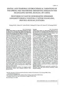
fluctuation magnitude, and its phase illustrates the peak time of the LST annual cycle. Figure 6 provides the 8-year (2003–2010) averaged mean LST on the Tibetan Plateau. The study area exhibits a highly contrasted spatial pattern of annual mean LST values, suggesting significant regional variabilities. The annual mean LSTs in most areas were generally within the range of 0 to 30uC, but some pixels were even larger than 30uC or lower than 0uC. Consulting the DEM map of the plateau (Figure 1), the spatial distribution of annual mean LST is influenced by the altitude. Areas with lower altitude generally have higher annual mean LST, indicating that higher altitude leads to lower temperature. The Qaidam Basin located in the northeast shows higher annual mean temperatures above 28uC due to its lower altitude and desert landscape. However, the annual mean LSTs of the South Tibetan Valley in the southwest, with relatively high altitudes ranging from 4500 to 5000 m, are also among the highest in the study area. This can be attributed to the area’s lower latitude and valley terrain and to the influence of the warm Southwest Monsoon. The Kunlun Mountains, located in the northwest, and the Nyainqentanglha Mountains, located in the south, show lower annual mean temperatures below 3uC. Large lakes in the plateau, such as Qinghai Lake and Nam Lake, also show relatively lower annual temperatures. Figure 7A and B represents the 8-year (2003–2010) averaged amplitude and phase, respectively, of the annual cycle of the LST series on the Tibetan Plateau. Figure 7A clearly reveals that the annual amplitude shows a spatial tendency that increases from the southeast to the northwest, which shows a similar spatial pattern with precipitation (Figure 7C). According to the surface heat balance, LST is controlled by solar radiation and surface thermal properties. High precipitation caused by the monsoon indicates heavy clouds, mainly in summer. The occurrence of clouds reduces solar radiation and in turn reduces the surface temperature, especially in summer. Lower summer temperatures decrease lower seasonal

12.14uC, which is also much higher than that of the second harmonic (2.86uC). This result suggests that the first harmonic (annual term with frequency 5 1) contributes far more to the overall LST time series than the second harmonic (semiannual term with frequency 5 2), indicating a strong unimodal periodic pattern of the LST temporal series on the Tibetan Plateau. The second harmonic contributes less to the overall fit but helps improve the HANTS fit performance. Spatiotemporal variations of LST

The HANTS simulation result of the LST time series is composed of the mean value of the LST temporal profile, amplitudes, and phases of the 2 harmonics. According to the preceding analysis, the mean and annual harmonic contribute more to the overall LST time series than the semiannual harmonic. Therefore, the 8-year (2003–2010) averaged mean LST and annual harmonic were used to represent the spatiotemporal variations of LST in the Tibetan Plateau. The mean term represents the annual mean LST value. The annual harmonic depicts the annual cycle of LST, its amplitude illustrates the seasonal


90


MountainResearch

FIGURE 6 Spatial distributions of the 8-year averaged annual mean LST of the Tibetan Plateau. (Map by Y. Xu)

fluctuations. Moreover, in this arid and semiarid area, higher precipitation usually results in higher vegetation cover and higher soil moisture, which are more resistant to seasonal oscillations of LST. Despite this general southeast–northwest difference, the most striking seasonal oscillation occurs at the Qaidam Basin, which is ascribed to its sparse vegetation cover, low soil moisture, and low altitude. The annual amplitude in this basin is usually higher than 15uC. In the Yarlung Zangbo Grand Canyon located in the southeast, the annual amplitude is mostly lower than 5uC, indicating slight seasonality. As the main water vapor channel of the Tibetan Plateau (Lin and Wu 1990), this area is highly influenced by the warm–humid Southwest Monsoon and shows a warm–temperate monsoon climate. Figure 7B demonstrates the spatial distributions of peak time for the LST annual cycle. Most of the study area has annual phase values ranging from 148 to 204 DOY, suggesting they achieve their peak value of the LST annual cycle at June and July.

FIGURE 7 Spatial distribution of the 8-year averaged (A) amplitude and (B) phase of the first harmonic in the Tibetan Plateau. (C) Precipitation map and (D) land cover map of the Tibetan Plateau. (Maps by Y. Xu)


91


MountainResearch

TABLE 1 General statistical results of the HANTS harmonic characteristics for each land cover type.

Land cover

Annual mean LST (6C)

Annual amplitude (6C)

Forest

16.62

9.48

174.40

Grassland

17.24

10.40

170.88

Water

6.75

10.02

200.95

Snow/ice

0.53

9.81

191.74

Bare land

18.00

15.63

181.12

Annual phase (DOY)

LST, land surface temperature; DOY, day of year.

amplitude of 15.63uC, due to its low heat capacity and low evapotranspiration. Grassland, water, and snow/ice show lower seasonalities, with amplitudes of 10.40, 10.02, and 9.81uC, respectively. However, forest exhibits the lowest seasonal oscillation, with an amplitude of 9.48uC. The lowest amplitude of forest is probably due to the evaporation and shelter effect of the vegetation canopy, which efficiently reduce temperature in growing season, especially in summer. For the phase of the first harmonic, grassland and forest show relatively lower respective values of 170.88 and 174.40 DOY, indicating that their maximum LSTs occur on June 19 and June 23, respectively. Forest and grassland show earlier peak times than other land types, which can be explained by the high cloud cover and high vegetation abundance in the growing season (from July to September) that reduce the summer temperature. Bare land reaches its peak LST on 181.12 DOY, approximately 10 days later than grassland. Snow/ice reaches its highest LST on 191.74 DOY, approximately 10 days later than bare land. Water shows the largest amplitude of 200.95 DOY, suggesting that its peak LST occurs on July 19. The lag effect of water surface temperature results from its high heat capacity.

In contrast to the amplitude, the spatial distribution of the annual phase does not present an obvious regular pattern, so it may be controlled by complex interactions of environmental variables, including solar radiance, underlying surface type, topography, vegetation abundance, climate, and soil moisture conditions. On the whole, the annual phase exhibits an inconspicuous southeast–northwest spatial tendency. The largest annual phases were found over large water bodies, suggesting that these areas have the latest peak time of LST due to their high heat capacities. High mountains, such as the Karakoram Mountains and Nyainqentanglha Mountains, also exhibit delayed peak times of LST for their permanent snow cover. Compared with the DEM map, there is an inconspicuous analogy between the spatial distributions of altitude and the annual harmonic, suggesting that altitude is not the decisive factor for the annual variations of the LST peak time. LST variations for different land cover types

To analyze the LST dynamic characters of the different land cover types in the study area, the original MODIS land cover map was reclassified by aggregating the 17 IGBP categories into 5 major land cover classes: forest, grassland, water, snow/ice, and bare land (Figure 7D). Based on the land cover map, the average values of the annual mean LST and the amplitude and phase of the first harmonic for each land cover type were calculated (Table 1). Table 1 shows that bare land exhibits the highest annual mean LST (18.00uC), followed by grassland (17.24uC), and forest (16.62uC). Vegetation cover has a dampening effect on LST due to the cooling effect of shading and evapotranspiration. For example, bare land displays a high temperature that can be related to its high insolation (caused by low cloud cover), low heat capacity, and lack of evaporative cooling (caused by low vegetation cover). In contrast, water displays a relatively low temperature because of its rather high thermal capacity and evapotranspiration. Thus, water shows a much lower mean temperature of 6.75uC, and snow/ice shows the lowest mean temperature of 0.53uC. For the amplitude of the first harmonic, bare land also shows the most distinct annual fluctuation of LST, with an


Conclusions In this paper, the spatiotemporal variations of daytime LST in the Tibetan Plateau were studied using AQUA MODIS 1-km LST data from 2003 to 2010. The harmonic analysis method HANTS was introduced to suppress cloud contamination and discriminate significant periodic variations of LST. Evaluation results indicate that the HANTS algorithm can provide satisfactory fitting for the LST time series and eliminate the influence of cloud cover on the remotely sensed LST data. The results of the HANTS analysis clearly show that the LST seasonal variation in the study area has a strongly unimodal periodic pattern. Therefore, most of the temporal variance was constrained to the mean term and the annual harmonic. The mean term of the harmonic analysis represents the annual mean LST value, which exhibits a significant regional variability in the study area. The spatial pattern of mean LST is generally influenced

92


MountainResearch

by the distributions of altitude and underlying surface. The amplitude of the annual harmonic describes seasonal fluctuations of LST and displays a remarkable southeast– northwest decreasing gradient, which corresponds to the distribution of precipitation. The phase of the annual harmonic describes the peak time of the LST annual cycle, which does not present such an obvious regular pattern as amplitude. Most of the area achieves its peak value of LST in June and July, and water bodies display the latest peak time. The geographic distributions of both seasonal fluctuation and peak time show little correspondence with altitude. The characteristics of the LST variations for different land cover types were also studied. Bare land shows the highest annual mean LST, followed by grassland, forest, water, and snow and ice. Bare land also exhibits the most prominent seasonal oscillations. Other land covers, such as grassland, water, and snow and ice, show lower

seasonalities relative to bare land, and forest exhibits the lowest seasonal fluctuation. For the annual phase, vegetation covers including grassland and forest show their early peak of the LST annual cycle. The bare land and the snow/ice classes reach their peak LST approximately 10 and 20 days later than grassland, respectively. Water shows the latest LST peak, representing an approximately 1-month lag compared with vegetation cover. This study gives spatially detailed information on the spatiotemporal variability of LST in the Tibetan Plateau, which is meaningful to understand the surface thermal condition and its influence on vegetation, frozen ground, and climate on the plateau. In addition, the HANTS algorithm is shown to be an effective approach for understanding the spatiotemporal variations of LST, especially for the regions with dense clouds that cause a large number of gaps in the LST data.

ACKNOWLEDGMENTS The authors thank the Land Processes Distributed Active Archive Center for providing MODIS land products and the US Geological Survey for providing SRTM3 DEM data. This research received financial support from the

Major State Basic Research Development Program of China (2011CB952002) and the National Natural Science Foundation of China (41201369 and 41001289).

REFERENCES

Lin Z, Wu X. 1990. A preliminary analysis about the tracks of moisture transportation on the Qinghai–Xizang Plateau [in Chinese with English abstract]. Geographical Research 9:33–40. Lin Z, Zhao X. 1996. Spatial characteristics of changes in temperature and precipitation of the Qinghai–Xizang (Tibet) Plateau. Science in China Series D 39:442–448. Liu X, Chen B. 2000. Climatic warming in the Tibetan Plateau during recent decades. International Journal of Climatology 20:1729–1742. Liu X, Cheng Z, Yan L, Yin Z. 2009. Elevation dependency of recent and future minimum surface air temperature trends in the Tibetan Plateau and its surroundings. Global and Planetary Change 68:164–174. Liu X, Yin Z, Shao X, Qin N. 2006. Temporal trends and variability of daily maximum and minimum, extreme temperature events, and growing season length over the eastern and central Tibetan Plateau during 1961–2003. Journal of Geophysical Research 111:D19109. Ma Y, Ishikawa H, Tsukamoto O, Menenti M, Su Z, Yao T, Koike T, Yasunari T. 2003. Regionalization of surface fluxes over heterogeneous landscape of the Tibetan Plateau by using satellite remote sensing. Journal of Meteorological Society of Japan 81:277–293. Manzo-Delgado L, Aguirre-Gomez R, Alvarez R. 2004. Multitemporal analysis of land surface temperature using NOAA–AVHRR: Preliminary relationships between climatic anomalies and forest fires. International Journal of Remote Sensing 25:4417–4424. Menenti M, Azzali S, Verhoef W, van Swol R. 1993. Mapping agro-ecological zones and time lag in vegetation growth by means of Fourier analysis of time series of NDVI images. Advances in Space Research 13:233–237. Oku Y, Ishikawa H, Haginoya S, Ma Y. 2006. Recent trends in land surface temperature on the Tibetan Plateau. Journal of Climate 19:2995–3003. Price JC. 1984. Land surface temperature measurements from the split window channels of the NOAA 7 Advanced Very High Resolution Radiometer. Journal of Geophysical Research 89:7231–7237. Qin Z, Berliner P, Karnieli A. 2001. A mono-window algorithm for retrieving land surface temperature from Landsat TM data and its application to the Israel– Egypt border region. International Journal of Remote Sensing 22:3719–3746. Qiu J. 2008. The third pole. Nature 454:393–396. Roerink GJ, Menenti M, Verhoef W. 2000. Reconstructing cloudfree NDVI composites using Fourier analysis of time series. International Journal of Remote Sensing 21:1911–1917. Salama MS, Van der Velde R, Zhong L, Ma Y, Ofwono M, Su Z. 2012. Decadal variations of land surface temperature anomalies observed over the Tibetan

Becker F, Li Z. 1990. Towards a local split window method over land surfaces. International Journal of Remote Sensing 11:369–393. Crosman E, Horel J. 2009. MODIS-derived surface temperature of the Great Salt Lake. Remote Sensing of Environment 113:73–81. Cuo L, Zhang Y, Wang Q, Zhang L, Zhou B, Hao Z, Su F. 2012. Climate change on the northern Tibetan Plateau during 1957–2009: Spatial patterns and possible mechanisms. Journal of Climate doi: 10.1175/JCLI-D-11-00738.1. de Jong R, de Bruin S, de Wit A, Schaepman ME, Dent DL. 2011. Analysis of monotonic greening and browning trends from global NDVI time-series. Remote Sensing of Environment 115:692–702. Ding Y, Zhang L. 2008. Intercomparison of the time for climate abrupt change between the Tibetan Plateau and other regions in China [in Chinese with English abstract]. Chinese Journal of Atmospheric Sciences 32:794–805. Du J. 2001. Change of temperature in Tibetan Plateau from 1961–2000 [in Chinese with English abstract]. Acta Geologica Sinica 56:690–698. Duan A, Wu G, Zhang Q, Liu Y. 2006. New proofs of the recent climate warming over the Tibetan Plateau as a result of the increasing greenhouse gases emissions. Chinese Science Bulletin 51:1396–1400. Friedl MA, McIver DK, Hodges JCF, Zhang XY, Muchoney D, Strahler AH, Woodcock CE, Gopal S, Schneider A, Cooper A, Baccini A, Gao F, Schaaf C. 2002. Global land cover mapping from MODIS: Algorithms and early results. Remote Sensing of Environment 83:287–302. Jiang H, Wang K. 2001. Analysis of the surface temperature on the Tibetan Plateau from satellite. Advances in Atmospheric Sciences 18:1215–1223. Jimenez-Munoz JC, Sobrino JA. 2003. A generalized single-channel method for retrieving land surface temperature from remote sensing data. Journal of Geophysical Research 108:4688–4695. Jin M, Dichinson RE, Vogelmann AM. 1997. A comparison of CCM2–BATS skin temperature and surface–air temperature with satellite and surface observations. Journal of Climate 10:1505–1524. Julien Y, Sobrino JA. 2010. Comparison of cloud-reconstruction methods for time series of composite NDVI data. Remote Sensing of Environment 114: 618–625. Julien Y, Sobrino JA, Verhoef W. 2006. Changes in land surface temperatures and NDVI values over Europe between 1982 and 1999. Remote Sensing of Environment 103:43–55. Li D, Zhong H, Wu Q, Zhang Y, Hou Y, Tang M. 2005. Analyses on changes of surface temperature over Qingha-i Xizang Plateau [in Chinese with English abstract]. Plateau Meteorology 24:291–298.


93


MountainResearch

Wang B, Ma Y, Ma W. 2012. Estimation of land surface temperature retrieved from EOS/MODIS in Naqu area over Tibetan Plateau. Journal of Remote Sensing 16:1289–1298. Wang W, Liang S, Meyers T. 2008b. Validating MODIS land surface temperature products using long-term nighttime ground measurements. Remote Sensing of Environment 112:623–635. Wang X, Zhong X, Fan J. 2005. Spatial distribution of soil erosion sensitivity in the Tibet Plateau. Pedosphere 15:465–472. Wen J, Su Z, Ma Y. 2004. Reconstruction of a cloud-free vegetation index time series for the Tibetan Plateau. Mountain Research and Development 24(4): 348–353. Westermann S, Langer M, Boike J. 2011. Spatial and temporal variations of summer surface temperatures of high-arctic tundra on Svalbard: Implications for MODIS LST based permafrost monitoring. Remote Sensing of Environment 115:908–922. WIST [Warehouse Inventory Search Tool]. 2011. http://wist.echo.nasa.gov/api/; accessed on December 16, 2011. Replaced by Reverb ECHO in 2012. http:// reverb.echo.nasa.gov/reverb/redirect/wist; updated on February 22, 2012. Xu Y, Ding Y, Li D. 2003. Climatic change over Qinghai and Xizang in 21st century [in Chinese with English abstract]. Plateau Meteorology 22:451–457. Yanai M, Li C, Song Z. 1992. Seasonal heating of the Tibetan Plateau and its effects on the evolution of the Asian summer monsoon. Journal of the Meteorological Society of Japan 70:319–351. Ye D, Gao Y. 1979. The Meteorology of the Qinghai–Xizang (Tibet) Plateau [in Chinese]. Beijing, China: Science Press. You Q, Kang S, Aguilar E. 2008. Changes in daily climate extremes in the eastern and central Tibetan Plateau during 1961–2005. Journal of Geophysical Research—Atmospheres 113:D07101. Zhong L, Su Z, Ma Y, Salama MS, Sobrino JA. 2011. Accelerated changes of environmental conditions on the Tibetan Plateau caused by climate change. Journal of Climate 24:6540–6550.

Plateau by the Special Sensor Microwave Imager (SSMI) from 1987 to 2008. Climate Change 114:769–781. Snyder WC, Wan Z, Zhang Y, Feng Y. 1998. Classification-based emissivity for land surface temperature measurement from space. International Journal of Remote Sensing 19:2753–2774. Tseng KH, Shum CK, Lee H, Duan J, Kuo C, Song S, Zhu W. 2011. Satellite observed environmental changes over the Qinghai–Tibetan Plateau. Atmospheric and Oceanic Sciences 22:229–239. Van De Kerchove R, Lhermitte S, Veraverbeke S, Goossens R. 2013. Spatiotemporal variability in remotely sensed land surface temperature, and its relationship with physiographic variables in the Russian Altay Mountains. International Journal of Applied Earth Observation and Geoinformation 20:4–19. http://dx.doi.org/10.1016/j.jag.2011.09.007. Verhoef W, Menenti M, Azzali S. 1996. A colour composite of NOAA–AVHRR NDVI based on time series analysis (1981–1992). International Journal of Remote Sensing 17:231–235. Wan Z. 2008. New refinements and validation of the MODIS land-surface temperature/emissivity products. Remote Sensing of Environment 112: 59–74. Wan Z, Dozier J. 1996. A generalized split-window algorithm for retrieving landsurface temperature from space. IEEE Transactions on Geoscience and Remote Sensing 34:892–905. Wan Z, Li Z. 1997. A physics-based algorithm for retrieving land-surface emissivity and temperature from EOS/MODIS data. IEEE Transactions on Geoscience and Remote Sensing 35:980–996. Wan Z, Zhang Y, Zhang Q. 2002. Validation of the land-surface temperature products retrieved from Terra Moderate Resolution Imaging Spectroradiometer data. Remote Sensing of Environment 83:163–180. Wang B, Bao Q, Hoskins B, Wu G, Liu Y. 2008a. Tibetan Plateau warming and precipitation change in East Asia. Geophysical Research Letters 35:702.


94
