and Iwao & Kuno (1971) was applied: mean crowding ?h = m + V/m - 1, where m and ...... random distribution in sets of parallel samples (Muus, 1967; Chambers ...
Helgol~inder wiss. Meeresunters. 32, 55-72 (1979)
Spatial configurations generated by motile benthic polychaetes* K. REISE Biologische Anstalt Helgoland (Litoralstation) ; D-2282 List~Silt, Federal Republic of Germany
ABSTRACT: Micro-spatial patterns of five infaunal polychaete species were investigated on tidal flats in the Wadden Sea (island of Sylt, North Sea). Sediment samples were taken within plots of 4 m2 at regular distances or with a multiple-cell corer composed of 144 contiguous units. Most of the configurations observed can be related to the mode of feeding. Individuals of the predatory polychaete Eteone longa do not generate discernible spatial structures. Anaitides mucosa, a carnivoruous scavanger, occurs in marked patches. Juveniles of Scoloplosarmiger, a burrowing deposit feeder, live in small aggregates which in turn conglomerate to larger ones. Adults are scattered within larger clusters. High density areas of juveniles and adults do overlap. Another burrowing deposit feeder, Capitella capitata, is even more aggregated. Local attractors may cause clusters of exceptional intensity. Territoriality is exhibited by the tube-dwelling surface deposit feeding Nereis diversicolor. The juveniles are restricted to interspaces left by the adults.
INTRODUCTION Dispersion of animals within benthi~c habitats has often been regarded as a nuisance to adequate sampling instead of a valuable source of ecological information. In recent years this attitude has changed. In a number of investigations multiple cell corers or other techniques of fine-scale regular sampling have been applied (Angel & Angel, 1967; Reys, 1972; Olsson & Eriksson, 1974; Rosenberg, 1974, 1977; Jumars, 1975; Help, 1976; Nixon, 1976; Gage & Coghill, 1977; Help & Engels, 1977; Jumars, Thistle & Jones, t977). Complicated statistics and the associated "body of assumptions" often are an encumbrance to spatial ecology. The conventional notion of randomness, manifested in the classification of spatial patterns into uniform, random, and clumped (i.e. Odum, 1971), is misleading. In ecological context, an "apparent randomness" is exceptable only, generated by a balance or a multitude of spatial variables. Random processes have never been shown to operate in the ecological world. The assumption of an uniform habitat is another outgrowth of statistical thought, devoid of ecological confirmation. Already the mere presence of organisms convert uniformity into heterogeneity. It is more helpful to envision local habitats as attractor surfaces relative to the organisms concerned. Such a surface consists of inhospitable regions and of domains of * I acknowledge a grant from the Deutsche Forschungsgemeinschaft (DFG).
56
K. Reise
local attractors, and organisms distribute accordingly. If these local attractors are defensible, regular spacing may occur between animals. Otherwise they will cluster. If animals are too few to generate a discernable spatial pattern, they are scattered. If they are densely packed and thus conceal the structure of the attractor surface, then their pattern is continuous. At intermediate numbers, animals are expected to generate compound spatial configurations, contingent upon their spatial behaviour and the environmental background space. In this paper, micro-spatial patterns of five motile polychaete species are analyzed and compared. Together they show an amazing complexity in their unfolding configurations. Structures seem to be predictable and most are related to the polychaetes feeding behaviour. Sampling was carried out on tidal flats in K6nigshafen, a sheltered bay of the island of Sylt (eastern part of the North Sea).
METHODS All sampling was done during low tide. To investigate spatial patterns of large worms, areas of 4 m 2 were subdivided into 64 units of '/,6 m 2. From the center of each areal unit a sample of 25 cm 2 • 20 cm depth was taken with a steel corer. Thus, there was a distance of 20 cm between adjacent samples. Sediment cores were transported immediately to the laboratory and were puddled through a 0.5 mm mesh sieve. Patterns of smaller worms, living close to the sediment surface, were obtained with a multiple cell corer of 24 x 24 cm outside dimensions, and 8 cm depth, composed of 144 contiguous 4 cm 2 units (Fig. 1). The corer is constructed of 0.5 mm steel. Because of its large surface area, it's challenging to push this sampling tool quickly into the sediment. The corer is placed in position and a metal-cover plate and a wood-block are put on top. A few powerful strokes on the block with a sledge hammer (usually) push the corer down to the desired depth of 8 cm. Immediately thereafter, the sediment surrounding the corer is removed as quickly as possible. A second metal-cover plate, with edges bent upwards along three of the sides, is pushed horizontally underneath the corer to prevent the downward escape of animals. When obstacles within the sediment prevented speedy action, the procedure was repeated at another place. Finally, the corer was closed with the cover plates and transported to the laboratory. The sediment was pushed out from each of the 144 cells separately with a strip of wood. To count animals, the sediment was diluted with sea-water in white plastic dishes. The small volume of cores made sieving superfluous. A third sampling method was adopted to reveal patterns of juvenile (< 5 mm in length) Scoloplos armiger (O. F. Miiller). A small metal plate was pushed horizontally through the sediment at a depth of I cm. 36 contiguous subsamples of I cm 3 were cut out with a paring knife and bottled. An attempt was made to keep the statistical analysis of the obtained spatial images as simple as possible. I believe that the complex indices "I and C" recently introduced into spatial ecology by Jumars, Thistle & Jones (1977) are a step in the wrong direction. Indices are inherently limited to measuring no more than one property accurately. If there are more spatial properties, these become averaged regardless of their qualitative differences. As shown in this study, spatial configurations of populations are generated by a compound
Spatial configurations
57
Fig. 1 ~Multiple cell corer to analyze micro-spatial patterns of polychaetes spatial behaviour. Thus, indices have to be used in a variety of specific ways to dissect the patterns into their spatial components ("individual treatment"). In this context, the analytical power of a single index is less important. Provided with a choice, I selected indices easy to handle but sensitive enough to keep statistical deformation within limits.
58
K. Reise
Primarily, the ?h-m methodology as proposed by Lloyd (1967), Iwao (1968, 1972), and Iwao & Kuno (1971) was applied: mean crowding ?h = m + V/m - 1, where m and V symbolize mean and variance. The index of patchiness, ?h/m "purports to measure how many times as crowded an individual is, on the average, as it would have to be if the same population had a random distribution" (Lloyd, 1967). A ratio ?h/m < 1 suggests regular spacing and ?h/m > 1 suggests clustering. Significant deviation from the assumption that neither one occurs is detected by introducing an appropriate chi-square, -m- = 1 + - - 1 (n-"~l - 1 ) , m m where n = number of samples. The index of patchiness is numerically quite similar to Morisita's index 16, hitherto more popular among benthic ecologists:
i/1 = I6 ( - ~ ) . To measure spatial autocorrelation (Cliff & Ord, 1973) between neighbouring samples, Iwao (1972) derived an index Q (rho), which indicates the ratio of the increment of ?h against m when adjacent samples are pooled to progressively larger areal units:
Q, =/hi - ?hi-i mi -- mi- 1' where i = 1, 2 . . . . stands for the order of areal size, and Q1 ?hl/ml. Because of the nested hierarchical design of areal units, the Q-values are not independent from each other, and changes in Q cannot be tested as to their significance. An alternative method for measucing the size of patches was suggested by Goodall, as outlined in Pielou (1977). From the grid with 144 cells, random pairs were picked, spaced apart at each of several chosen distances. I only used distances in vertical and horizontal directions. From each pair the variance was estimated. For the sequence of center-to-center distances of 2, 4, 6, and8 cm I calculated 100 variances each time. Since the averaged variances were mutually independent, standard statistical methods can be used to test the significance of differences (Pielou, 1977). To measure spatial interaction between subpopulations, I superimposed one pattern upon the other. First, the index of patchiness was calculated from the real compound pattern. Then, one pattern was rotated and indices were calculated at distortions of 90 ~, 180 ~, and 270 ~. In the absence of any spatial correlation between patterns, no marked differences emerged between the real and the distorted juxtapositions. In the case of a positive correlation, the ?h/m-value obtained from the real pattern would be higher than the others. If it is lower, spatial segregation occurs. There is one shortcoming in this method. If patterns exhibit symmetrical properties, the distorted configurations will depend on the type of symmetry. In natural patterns of animal populations, however, the chance of symmetry is rather low. In the following, * denotes p = 0.05 significance, ** 0.01, and *** 0.001. =
RESULTS The predatory phyllodocid Eteone longa (Fabr.) normally burrows in the sediment, although it is often found crawling on the surface (Rasmussen, 1973). Behrends &
Spatial configurations
59
Michaelis (1977) observed it in pursuit of Scolelepis squamata (Miiller) tearing off pieces from the victim's hind end. Two 4 m 2 plots were selected on sand flats. 64 regularly spaced samples were taken as described from each. The obtained spatial images contained 17 and 20 worms respectively. None of the applied analytical tools was able to detect any significant deviation from a free configuration. Apparently, the worms were scattered over the two plots and their spatial behaviour did not generate an observable structure. Anaitides mucosa (Oersted), another phyllodocid, is primarily a carnivoruous scavanger. Dead bivalves and decaying shore crabs attracted several worms. This could easily be observed on the sediment surface. Mucuous trails were leading to and from carrion in a starshaped manner. During bright daylight this activity ceases, it is however easy to observe on a cloudy day or during the night. On one occasion (9.5. 1974, 23.00) up to 38
Fig. 2: Spatial configuration of Anaitides rnucosa in a sand flat; 64 regularly spaced samples within 4 m2 worms were counted gathering around a dead shore crab. Furthermore, crushed cockles and mussels placed on the sediment surface attracted numerous worms within a few minutes. If this mode of feeding is the prevailing one, worms are expected to cluster at a few locations provided with carrion. This is confirmed by the 64 regularly spaced samples within a 4 m 2 area of a sand flat (Fig. 2). Lloyd's index of patchiness denotes marked clusters (m = 0.7, l~/m = 6.5***). In the one sample with 13 worms, remains of a shore crab were found. Scoloplos armiger (O. F. Miiller) is a burrowing deposit feeder. It selectively takes up sand grains with its proboscis. Burrows are clearly visible in the sediment, but seem to be only semipermanent. Primarily, adult worms dwell in the upper 10 cm of the sediment. In February, out of 131 adult worms, I found 51 ~ at a depth of 0-5 cm, 37 % at 5-10 cm, and the remaining 12 % at 10-15 cm. Juveniles are confined to the upper 5 cm. A fine-scale vertical analysis was carried out in June. At this time, juveniles attained a length of 5 ram. The layer between 4 and 10 mm waspreferred (Table 1). Although juveniles avoid the
60
K. Reise
sediment-water interface, they remain above the zone occupied by the adults. Of course, as the young worms grow they gradually shift to deeper layers. During winter they join the pattern of the adults. Table 1 Vertical distribution of juvenile and adult Scoloplos armiger in the upper 5 cm of a sand flat (indiv. 25 cm-2) Depth (mm)
Juveniles
Adults
o-2 2--4 4-6 6-8 8-10 10-20 20-30 30-40 40-50
0 8 38 93 61 22 1 0 1
0 0 0 0 0 0 4 2 1
In September (5.9.1977) the horizontal dispersion of S. arrniger was investigated with 64 regularly spaced samples within 4 m 2 of a sand flat. I recognized two size classes: < 15 mm and 30-60 mm in length. The smaller ones represent the juveniles which hatched from their cocoons the preceeding spring. Both patterns are patchy (Fig. 3). In the adult worms, clusters are not at all obvious, except for the one sample containing nine individuals (fig. 3 B). Accordingly, the exclusion of this sample results in a pattern not discernible from a free configuration by the index of patchiness (real pattern: m = 2.23, ~ / m - 1.16"; without the '9-individual sample': m = 2.13, l~/m = 1.04). The striking feature is that samples with 0, 1,2, 3, and 4 worms have nearly the same frequency (10-13). Such a distribution is unlikely to be generated by a random process. On another sand flat, I
A
B
Fig. 3" Spatial configurations of Scoloplos arrniger on sand flats; 64 regularly spaced samples within 4 m2; A: juveniles (< 15 mm), B: adults (30-60 ram)
Spatial configurations
61
found only 19 adult individuals within a 4 m 2 grid. All but two individuals were confined to the left half of the grid. An analysis of this part of the grid revealed no patchiness (m = 0.53, ~ / m = 1.41). This grid indicates the existence of large scale patches, lacking internal structure. The spatial pattern of the juvenile S. armiger (Fig. 3 A) is strongly aggregated (m = 2.44, ~ / m = 2.00***). This patchiness is apparent even at a larger scale. All samples were arranged into 16 groups, each containing four adjacent samples: m = 9.75, ~ / m = 1.20"**. The grid with abundant juveniles and adults (Fig. 3 A, B) was divided into four 1 m2-units, each containing 16 samples. For each set "mean crowding" was calculated. The m-on-m relations for these four subunits are shown in Figure 4. While ~ -
8-
/
o
/// / / / / / / / / /
o a o
/ /
a /
/
/
/
/
/ / // /
/
/
rn
Fig. 4: ~-on-m regression for adults (/X), juveniles (Q), and the combined (O) population of Scoloplos armiger inhabiting 4 m2 of a sand flat; broken line: ~ = m values for the adult population remained close to unity, those of the juveniles and of the combined population are more or less remote from the ~ = m line. If high density areas of juveniles and adults alternate, ~l-values of the total population should be similar to the mean. This is apparently not the case. To find out whether the opposite is true, i.e., whether high density areas coincide, one configuration was superimposed upon the other, and the method of pattern rotation was applied. The highest degree of patchiness was obtained from the real pattern: 1.42 as opposed to 1.27 + 0.07. This indicates significant overlap between high density areas of the two subpopulations. In August (12.8. 1977), the horizontal distribution of juvenile S. armigerwas analyzed on a much smaller scale. The multiple cell corer composed of 144 contiguous 4 cm 2 units was pushed 8 cm deep into the sediment. The juvenile worms were with 279 individuals within the grid, and showed a spatial configuration of high structural complexity (Fig. 5). As a first step of analysis, the grid area of 576 cm 2 was divided into nine subareas of 64 cm 2. Thus, each subarea contains 16 cells. "Mean crowding was calculated for all subareas and the ~ - o n - m regression is shown in Figure 5 B. One value implied an
62
K. Reise
9 , . . . . . .
9
"
~ 1 4 9
~
9
,
9
,,
,.'.,..,.'.,
9 9 .
~ .
.
.
.
9
,
9
,
,
,
9
4
,
. .. :.: .: ....,.'.,:..,
:~.."
. . . .
:.....
~i.'.
~
~
~
9" .'.l.': .......... : : I Z ~ "i:
.........
i!i " 9 ".i.
"
"
/
1/11
"" :: ....
"
9 9 /I// /
/
.~:~
/
9
A
Spatial configuration of juvenile ( < 10 m m ) Scoloplos an'niger; A : 144 contiFuous cells of 4 c m 2, B: ~-on-m regression for 9 subunits composed o f 16 cells, 1 s u b u n i t ( ) is not taken into account by the calculated regression line, broken line:/!fi = m Fig. 5:
outstanding degree of aggregation which was caused by a singular aggregate within a low density area. This clump was positioned at the edge of the corer, and therefore should not be given too much weight9 Still, it might have been a "spatial sponge" soaking up individuals from its neighbourhood. For the remaining eight values the regression line was calculated ( ~ = 0.3 + 1.2 m), exhibiting a positive intercept and a slope larger than one. This indicates an overall patchiness and is confirmed by a highly significant index of patchiness for the total grid (m = 1.94, ~ / m = 1.61::'*::'). What is the size of these patches and how are they arranged? These questions demand a measure of spatial autocorrelation. The simplest approach is to plot m versus m with successively increasing areal units. From the basic units of 4 cm 2 on, the m-on-m regression remains well above the ~ = m line, with an increasing degree of divergence (although not uninterrupted). This implies small-sized aggregates which conglomerate into loose patches :b
8-
T
V
14-
1.2"
1.0-
0.8-
~i
$ A
~'6
2',*
3'8 ,*'8 8',* cm 2
~
~ B
~ cm
Spatial autocorrelation in juvenile Scoloplos armiger; A: o-indices with successive changes in scale, B: Goodall's variability for successive distances between cells, the standard error of the estimated average is indicated Fig. 6:
Spatial configurations
63
on a larger scale. Plotting the Q-indices against an increasing size of areal units yields a rather irregular curve (Fig. 6 A). As the Q-index is most sensitive to changes in spatial structure, relative to scale, this behaviour suggests that larger patches have no distinct shape and size. Q-indices approach unity, if the pattern is chaotic. This is not the case. Apparently, density varies from location to location in a non-random, complex manner, without any simple regularity. This conclusion is confirmed by a third measure of spatial autocorrelation, Goodall's method of random pairs of spaced samples9 With increasing distance between paired samples, there are definite changes in variability (Fig. 6 B). Variance is particularly low at a center-to-center distance of 6 cm. This corresponds well to the marked decline of Q-values between areal units of 36 and 48 cm 2, and indicates an average patch size of 36-48 cm 2, in addition to the small patches of 4 cm 2. In July (13.7. 1977), when juveniles were still < 5 mm in length, a grid as small as 36 cm 2 was divided into 36 units of 1 cm 3 each. The 15 worms found assembled into two distinct groups of 6 and 9 individuals9 This picture confirms the existence of fine-scale patches. The direct development of juveniles in cocoons may be in part responsible for the observed patchiness. Preferentially, juveniles leave the cocoon through the vertical stalk. This enables them to colonize the neighbourhood without becoming exposed to disrupting currents at the bottom surface. In addition, the egg cocoons are positioned in aggregates themselves. An area of 144 contiguous units of 100 cm 2 was sampled in April (4. 4. 1978)9 Egg cocoons were assembled in small patches between 900 and 1600 cm 2 in size (Fig. 7). Capitella capitata (Fabr.) is another burrowing deposit feeder9 This species is well known for popping up in large numbers wherever sewage runs into the sea. Worms live in tubes and also move about in the sediment. What they preferentially do on the flats investigated, I don't know. In the following, spatial configurations of small (< 15 mm in
9 I, 9
:...'.
::
,9
9
9 .
9 16
14-
1.2-
,,
,
',
. 08-
:i' I
9 A
:i: ...........
100 B
i
200
I
400
i
i
900
1600 cm 2
Fig. 7: Spatial configuration of egg cocoons from Scoloplos armiger; A: 144 contiguous cells of 100 cm,2 B: Q-indices with successive changes in scale length) and large (> 30 ram) worms are represented9 As the small individuals had already reproduced, they do not represent the juvenile group of the larger ones. They may be two separate species (see Grassle & Grassle, 1976)9
64
K. Reise
Samples taken from a 4 m 2 plot of a sand flat contained 93 large individuals. Small ones were not counted because not all of them were retained by the sieve mesh size 0.5 mm. There was strong evidence of patchiness (m = 1.45, ~ / m = 1.85"**). Samples containing 5 or 6 worms exceeded by far the frequencies likely to be produced with a Poisson model. Patchiness was still indicated when samples were arranged into 16 groups, each composed of four adjacent samples (m = 5.80, ~ / m = 1.22"*). This suggests loose patches, at least ~/4 m 2 in size. The spatial configuration of small C. capitata was investigated with the multiple cell corer (Fig. 8). At a first glance, this portrait looked quite erratic with two exceptional aggregates at the edges. However, the configuration was highly structured. As a first step of analysis, the grid was divided into nine subareas, each composed of 16 cells. Only two subareas which happened to include an exceptional aggregate (7 or 10 worms) contained a discernible patchy distribution. They cause an aggregated pattern for the total grid area (m = 0.88, r~/m = 2.12"**). Plotting ~ versus m for these nine subareas yielded a rather strange regression line ( ~ = - 1.5 + 3.4 m; r = 0.97**). The negative intercept with the k-axis, while the slope is ~> 1, suggests the existence of two opposing spatial structures. At low densities, there is a tendency toward regular spacing between individuals, while high densities are correlated with strong aggregates. As the next step in pattern analysis, the index 0 of spatial autocorrelation was plotted against the increasing scale in order to get an idea about the size of high density areas and about the dispersion within them (Fig. 9 A). As was to be expected, the 0-index for the smallest units indicated pronounced patchiness. However, this was entirely caused by the two elite structures at the edges. When these were excluded from the calculation (open circles in Fig. 9 A) spacing is suggested within clusters of 8-24 cm 2 in size. These clusters seemed to conglomerate into patches larger than 36 cm 2, as was indicated by the second peak in the 0-curve. Goodall's method of spaced samples within random pairs was of limited sufficiency when applied to this spatial configuration, because overall density is rather low, relative to the local overload in two of the cells (Fig. 9 B). These aggregates cause the standard error of the estimated average variability to be extremely large. The exclusion of these two elite structures results in a phenomenon similar to that shown for the 0-indices. Adjacent cells are similar (low value for 2 cm distance). The comparatively low variance for cells at a 6-cm distance suggests patches at this scale, and corresponds to the second peak in figure 9 A. To sum up, there seems to be a basic configuration of spaced worms within small patches. These patches conglomerate into larger ones. Superimposed on this pattern are two exceptional aggregations that possibly drain individuals from their neighbourhoods. In the grid from the sand flat, I found 127 small C. capitata. Another grid, this time from a mud flat, contained 294, small worms (Fig. 10). It was apparent that the lower left part of the grid was only occupied by some scattered individuals. This obstacle introduced an additional source of variability into the spatial pattern. However, it is quite similar to the basic configuration found in the population of the sand flat. Dividing the grid into nine subareas, again reveals no more than two areas which include a patchy dispersion of worms. This time, patchiness was not caused by local overload. Still, the ~ - o n - m regression plotted for the nine subareas has a negative intercept and a positive slope as in the sand flat population: ~ = - 0 . 3 7 + 1.42 m; r = 0.85**. Equally, the 0-indices
Spatial configurations
65
suggest a similar pattern: small patches conglomerate to larger ones (Fig. 11 A). Even more striking is the similarity revealed by Goodall's method (Fig. 11 B). The variability between spaced cells of selected distances is alike in both populations, provided the two exceptional aggregations in the sand flat grid are excluded9
9
"
9 - 9149
9
9
"
".:.i
9
Fig. 8: Spatial configuration of small (< 15 mm) Capitella capitata in a sand flat; 144 contiguous cells of 4 cm2
2.0-
~
,
1.5-
lo_
9
A
0.5-
cm 2
B
cm
Fig. 9: Spatial autocorrelation in small Capitella capitata in a sand flat; A: Q-indices with successive changes in scale, open circles: two exceptional clusters are excluded, B: Goodall's variability for successive distances between cells, the standard error of the estimated average is indicated, open circles as in A
66
K. Reise ,9
9
9
,,
,,
.
,.
9
.
.
. . . . . . . . . . . . 9 .i.:li~J.-i.'.
.
.
9 : ....
-i:,:
i:..i ........
9 .'. ........... 9 .-,": 9
:"
"
, . . , .
,,
. . . . . . . . . .
.
:lii
:." .......
:i:
": ::iii ,
,
, . : ,
i
9
i
9
,.
~
,
9 i
.
.
,~.
9
.'.
.......
i
.
, , ,
9
.
i
" 9
9
.9
.
.
.
.
9
"
.
.
! 9
.': 9 ,,.
,
i.i.:..:..:.-i..,} I
.
.
-:."
.'q
Fig. 10: Spatial configuration of small (< 15 mm) Capitella capitata in a mud flat; 144 contiguous cells of 4 cm2
7
/ 1.0
. . . . . . . . . . . . . . . . . .
A
e ~
cm
2
B
cm
Fig. 11: Spatial autocorrelation in small Capitella capitata from a mud flat; A and B as in Fig. 9
Unlike the other polychaetes mentioned above, Nereis diversicolor O. F..Miiller dwells in a permanent tube. However, occasionally worms are found crawling upon the bottom or even swimming in the water above. Goerke (1966) and Muus (1967) reviewed the 13olythetic feeding behaviour of this species which may be a deposit feeder, a herbivore, a predator, and a scavanger. Primarily, N. diversicolor seems to be a surface-deposit feeder. At least in the area investigated, branching feeding tracks surrounding the entrances of burrows support this view. Retreat-tubes of large worms may have two or more openings to the surface9 Worms usually stay with their tail ends in the burrow while feeding, and retract quickly when disturbed9 On a sand flat, 64 samples were taken from a 4 m 2 area in September (1.9. 1977). The obtained spatial patterns for small (20-60 mm) and for large (> 60 mm in length) worms are shown in Figure 12. The spatial configuration of small N. diversicolor was patchy (m = 1.64, m/m = 1.26"'). When samples were divided into 16 groups of four adjacent samples, patchiness was no longer discernible (m = 6.56, m/m = 1.03). Large worms did not aggregate (m = 0.95, ~ / m = 0.99)9 At the scale of four adjacent samples the configuration became more even (m = 3.81, (fi/m = 0.96). The combined pattern of both size classes was devoid of aggregation as well ( ~ / m = 0.98). To find out whether the plot of
Spatial configurations
67
4 m z contained different spatial components, four subareas of 1 m 2 were analyzed separately. Small worms in the upper right quarter of the grid were the only ones to show significant aggregation (m = 1.88, ~ / m = 1.60"*). All others were scattered. Is there some spatial interaction between the patterns of small and large worms? To get an answer, one configuration was rotated upon the other and the A/m-indices were calculated. It is evident that the real position yielded the most even configuration (real pattern: i~/ m = 0.98, distorted patterns: ~ / m = 1.13 + 0.06). Apparently, the patches of small worms are to some degree confined to the interspaces left by the large worms.
B
Fig. 12: Spatial configurations of Nereis diversicolor on a sand fiat; 64 regularly spaced samples within 4 m2, A: small (20-6C mm), B: large (> 60 mm) worms In August (30.8. 1977), a grid of 144 contiguous 4 cm 2 units was obtained from the same sand flat to study the dispersion of juvenile N. diversicolor (Fig. 13). At that time their length varied between 5 and 10 mm. N o obvious structures were apparent in the spatial configuration. Dividing the grid into nine subareas and analyzing the spatial configurations within these areas, gave no evidence of patchiness. Six areas contained configurations which suggest uniformity. However, the values were wildly scattered. Changes of e~indices using an increasing scale did not suggest much spatial structure either (Fig. 13 B). At a smaller scale, individuals were scattered or uniform, at a larger scale, some heterogeneity was indicated. The lack of spatial structures at the neighbourhood scale resembled the configuration of large worms (fig. 12 B). Even between these juveniles some regular spacing probably occurs. In the following year (5.6. 1978) most of these juvenile worms attained a length of 4 to 6 cm. During low tide, but with a sediment still covered by a thin layer of water, it was easy to detect the burrow entrances of these worms. Grids of 64 contiguous squares of 16 cm 2 each were superimposed on the flat and the entrances were counted (Fig. 14). I deliberately selected plots of high uniformity in surface texture to keep environmental "background noise" as low as possible. Density never exceeded four entrances per square. Thus, the territories in this population covered areas of at least 4 cm2. This
K. Reise
68
:: PIll o.
o
12
I
::
"i
.
.
.........
.
.
I
4
8
16
24
B
A
36
48 64 cm ~
Fig. 13: Spatial configuration of juvenile (5-10 mm) Nereis diversicolor in a sand flat; A: 144 contiguous ceils of 4 cm2, B: 0-indices with successive changes in scale
9
~
~176176 ~
~
o~176
~176
..I.. ~176 ~176
I
@
m
I
i
. ~
9
.
.
.
~
9
o
~176176
I
*~176 9 9
e
I
e
~
.o
m
9
~
81
9
~
~176 9
~
9
9~
I o
~176
~176176
" 9
........
99
~
~
"
~
~176
~
~
"
9
~176
~
~
~
. . . .
~
,~176 ~ ~
~ ~176
,::..'..
~
"~
~
"~
,'.',.'.,:.:,
~
"~
,
~
i'J--i
108
~176
~
i
111
~
' ~ 1 7 6
~
~ ~
~
~ 1 7 6
~ 1 7 6
~
~176
~
~
~176 .~
r... :.: :':.....
.. "4""i
.
.
.
*
.
. . . . . . . . . . . . . 126
~ i ~ 1 7 6 1 7 6 1 7 6l o ~ 1 7 6 1 7 6 1 7 6 1 7 6
: .........
..I.. 136
Fig. 14: Spatial configurations of burrow entrances of Nereis diversicolor in a sand flat; six grids, each with 64 contiguous ceils of 16 cm2; the numbers refer to entrances per grid
Spatial configurations
69
corresponded well to the observed length of feeding tracks which rarely extended to more than 1.5 cm from the entrances of the Vertical tubes. For all six grids, the ~ m - r a t i o remained well below unity and the pattern deviated significantly (p < 0.001 in all cases) from apparent randomness. The highest degree of regular spacing was realized at the highest density of tubes (136 entrances 1024 cm -2, m = 2.125, r ~ m = 0.695; the 0.99 significance limit: 0.813). This pattern strongly indicates that N. diversicolor maintains defended territories surrounding its burrows.
DISCUSSION Generally, it is impossible to obtain the pure spatial patterns of cryptic infaunal polychaetes. Deformations are inevitable. First of all, the three-dimensional patterns are compressed to plane patterns. This is negligable in N. diversicolor because its food resource is confined to the sediment surface. The limited resolving power of a grid composed of squares contributes to further deformations, i.e., quadrats cut through the edges of irregular shaped clusters. This will lower the contrast in the observed spatial image. All investigations were carried out during low tide. I do not know how such "snapshots" are related to the dynamic patterns of these motile polychaetes. The total deformations may be considered as additive noise, introducing a chaotic element and thereby tend to destroy structures (Grenander, 1976). On the other hand, inadequate statistical tools may produce spurious structures, sometimes difficult to disentangle from the real ones. With these considerations in mind, let us discuss the presented spatial configurations. E. longa is the only species lacking discernable spatial structures in the population investigated. This may be due to the rather low density, 106 and 125 worms m -2, i.e., on the average 94 and 80 cm 2 bottom per individual. However, it is unlikely that worms do not encounter each other at this density. Instead, I assume, that they just do not interact in a way to generate a discernible spatial configuration. This is quite reasonable for a predator, chasing its victims at high speed through the sediment to bite off their hind ends. The other phyllodocid species, Anaitides mucosa, generates clusters of high intensity. This is to be excepted for a carnivoruous scavanger, feeding on carrion like that from shore crabs and cockles. Preying on small worms, as is reported by Rasmussen (1973), is not consistent with the observed configuration. Thus, spatial analysis is able to indicate which of the two modes of feeding predominates currently. Patches in populations of S. arrniger have been reported previously (Reys, 1972; Gage & Coghill, 1977). From their studies, patches of less than I m 2 or of a diameter of 20-40 cm can be inferred. In the tidal populations presented here, adults may show large patches on a m 2 scale. On a fine-scale, only one exceptional patch could be observed. Otherwise, a mosaic of slightly different densities is apparent. Such a pattern is likely to be generated in response to a heterogeneous food resource spectrum. Juveniles of S. arrniger, on the other hand, are clearly aggregated. Ripplemarks, cockles, epibenthic predators, casts and funnels of lugworms are all sources of spatial heterogeneity preferentially affecting the juvenile worms which remain close to the sediment surface. In addition, juveniles start off from a patchy pattern when hatching from an egg cocoon. This nursery induced patchiness is still more amplified by the patchy
70
K. Reise
dispersion of cocoons themselves. This might have a lasting effect on juvenile dispersion. The gut of S. armiger always contains relatively few sand grains. Most probably, it is feeding on certain bacteria adherent to these sand grains. The dispersion of this food resource may be responsible for the basic pattern of juveniles and adults. At least, the compound mosaic of densities is not likely to be generated by gregariousness. The fact that high density patches of adults and juveniles overlap, support the hypothesis of a variable food resource constraining the pattern. However, the internal structure within large patches of juveniles is hardly to be explained with food availability. Some other spatial variables are more likely to contribute to this polymorphic arrangement. Spatial configurations in Cap#ella capitata are even more complex and clusters are of higher intensity. The occurrence of patchiness in populations of C. capitata is well known (Reys, 1972; Rosenberg, 1972; Gage & Geekie, 1973; Warren, 1977). In laboratory experiments, designed by Augustin & Anger (1974), worms were attracted to dead organic matter. Nevertheless, field investigations carried out by Warren (1977) did not demonstrate a positive correlation between organic matter and abundance. Probably, the analysis should be carried out at the level of bacteria. As a source of patchiness in juveniles, Warren (1977) suggests the direct development in maternal tubes, from which worms may enter the surrounding sediment without disrupting dispersal. Thus, patches of juvenile C. capitata and S. armiger can be generated by a similar process. However, the two exceptional aggregates found in the sandflat population of small worms are not composed of a single size class. This makes their origin from a common maternal tube unlikely. In the basic pattern, worms do not aggregate at the scale of single cells. This would be expected if attraction between individuals is part of their spatial behaviour. The only explanation left for the occurrence of the local overload in two instances is a localized, highly desirable, food resource, recognizable from some distance apart. In general, the spatial configuration of C. capitata is more patchy than that of S. armiger. Both species seem to feed on bacteria. The former utilizes bacterial growth on decaying organic matter, while the latter selects bacteria growing on sand grains. The distribution of decaying organic materials is certainly more patchy than sand grains are. Thus, it seems to be possible to predict food requirements from spatial analysis. Unlike other benthic polychaetes, N. diversicolor shows an even or apparently random distribution in sets of parallel samples (Muus, 1967; Chambers & Milne, 1975). This is confirmed by the present study. Moreover, I suggest territoriality among these surface deposit feeding worms. There are general reasons why spatial exclusion is most difficult to detect from spatial images presented as counts per unit area. Territorial animals respond to habitat heterogeneity just as other animals do. If there are few attractive basins in a local area, and each basin is large enough to provide space for several territorial worms, then the pattern will look patchy unless the sampling units match the size of the individual territories. Ideally, even the shape of the sampling units should be similar to that of the territories in order to detect regular spacing. Whatever their shape, they are unlikely to be quadratic as multiple cell corers usually are. There are two spatial aspects of territoriality in N. diversicolor. First, within age groups, worms do not generate discernible patches on the neighbourhood scale although population density is rather high, and burrow entrances are spaced regularly. Second, juvenile occurrence is restricted to interspaces left by the larger worms. Thus, the general
Spatial configurations
71
spatial configuration seems to be a nested-in territoriality. Muus (1967) observed " . . . the lightning speed of retreat when Nereis encounters other N e r e i s . . . " , and it is easy to conceive the defence of feeding areas by the powerful jaws on the evertable proboscis. Regular spacing in animals of marine soft sediments is not a common phenomenon. Paradoxically, the very first investigations in marine spatial ecology described just this type of configuration (Holme, 1950; Johnson, 1959; Connell, 1963). Most of their examples are surface deposit feeders. In comparing the spatial configurations found in the five motile polychaetes, feeding behaviour seems to be the primary cause of pattern formation. Brood protection with subsequent direct colonization of the surrounding sediment may have a lasting influence on juvenile patchiness. Clusters in juvenile N. diversicolor are caused by the territorial demands of adult specimen. Gregariousness has been demonstrated for a number of benthic animals. Yet, I do not think that I found any evidence for such social behaviour. Aggregations due to mating do occur in A. mucosa (Sach, 1975). However, the time of my investigation was unsuitable to observe mating behaviour in one of the polychaete species concerned. The most general aspect of this study is that intertidal polychaetes apparently do not experience an environment where plentiful food is just everywhere. They either have to chase their prey, cluster where desirable food is available, or have to defend a limited supply.
Acknowledgements. Laboratory space and research facilities were provided by the Biologische Anstalt Helgoland and the 2. Zoologisches Institut, Universitiit GSttingen. Particular thanks are due to Mr. E. Jordan who constructed the multiple cell corer, to Mr. R. v. Sivers who prepared the art work, and to Mrs. D. Biirger who processed the photographs.
LITERATURE CITED Angel, H. H. & Angel, M. V., 1967. Distribution pattern analysis in a marine benthic community. Helgoliinder wiss. Meeresunters. 15, 445-454. Augustin, A. & Anger, K., 1974. Experimente iiber Substratpr~iferenzen von Capitella capitata (F.). Kieler Meeresforsch. 30, 28-36. Behrends, G. & Michaelis, H., 1977. Zur Deutung der Lebensspuren des Polychaeten Scolelepis squamata. Senckenberg marit. 9, 47-57. Chambers, M. R. & Milne, H., 1975. Life cycle and production,of Nereis diversicolor in the Ythan estuary, Scotland. Estuar. coast, mar. Sci. 3, 133-144. Cliff, A. D. & Ord, J. K., 1973. Spatial autocorrelation. Pion, London, 178 pp. Connell, J. H., 1963. Territorial behaviour and dispersion in some marine invertebrates. Res. Pop. Ecol. 5, 87-101. Gage, J. D. & CoghiI1, G. G., 1977. Studies on the dispersion patterns of Scottish sea loch benthos from contiguous core transects. In: Ecology of marine benthos. Ed. by B. C. Coull. Univ. of South Carolina Press, Columbia (Belle W. Baruch Lib. Mar. Sci. 6,) 319-337. - - & Geekie, A. D., 1973. Community structure of the benthos in Scottish sea-lochs. II. Spatial pattern. Mar. Biol. 19, 41-53. Goerke, H., 1966, Nahrungsfiltration von Nereis diversicolor O. F. Miiller (Nereidae, Polychaeta). VerSff. Inst. Meeresforsch. Bremerhaven 10, 49-58. Grassle, J. & Grassle, J. F., 1976. Sibling species in the marine pollution indicator Capitella (Polychaeta). Science, N. Y. 192, 567-569.
72
K. Reise
Grenander, U., 1976. Pattern synthesis. Lectures in pattern theory Springer, New York 1, 1-509. Help, C., 1976. The spatial pattern of Cyprideis torosa (Jones, 1850) (Crustacea, Ostracoda). J. mar. biol. Ass. U. K. 56, 179-189. - - & Engels, P., 1977. Spatial segregation in copepod species from a brackish water habitat. J. exp. mar. Biol. Ecol. 26, 77-96. Holme, N. A., 1950. Population dispersion in Tellina tenuis da Costa. J. mar. biol. Ass. U. K. 29, 267-280. Iwao, S., 1968. A new regression method for analyzing the spatial pattern of animal populations. Res. Pop. Ecol. 10, 1-20. 1972. Application of the ~-m method to the analysis of spatial patterns by changing the quadrat size. Res. Pop. Ecol. 14, 97-128. & Kuno, E., 1971. An approach to the analysis of aggregation pattern in biological populations. In: Statistical ecology. Ed. by G. P. Patil. Pennsylvania State Univ. Press, University Park, P. A., 1, 461-513. Johnson, R. G., 1959. Spatial distribution of Phoronopsis viridis Hilton. Science, N. Y. 129, 1221. Jumars, P. A., 1975. Environmental grain and polychaete species' diversity in a bathyal benthic community. Mar. Biol. 30, 253-266. - - Thistle, D. & Jones, M. L., 1977. Detecting two dimensional spatial structure in biological data. Oecologia 28, 109-123. Lloyd, M., 1967. "Mean crowding." J. Anim. Ecol. 36, 1-30. Muus, B. J., 1967. The fauna of Danish estuaries and lagoons. Meddr Danm. Fisk. -og Havunders. 5, 1-316. Nixon, D. E., 1976. Dynamics of spatial pattern for the gastrotrich Tetranchyroderma bunti in the surface sand of high energy beaches. Int. Revue ges. Hydrobiol. 61, 211-248. Odum, E. P., 1971. Fundamentals of ecology. Saunders, Philadelphia, 574 pp. Olsson, I. & Eriksson, B., 1974. Horizontal distribution of meiofauna within a small area, with special reference to Foraminifera. Zoon 2, 67-84. Pielou, E. C., 1977. Mathematical ecology. Wiley, New York, 385 pp. Rasmussen, E., 1973. Systematics and ecology of the Isefjord marine fauna. Ophelia 11, 1-507. Reys, J. p., 1972. Analyses statistiques de la microdistribution des esp~ces benthiques de la r~gion de Marseille. Tethys 3, 381-403. Rosenberg, R., 1972. Benthic faunal recovery in a Swedish fjord subsequent to the closure of a sulphite pulp mill. Oikos 23, 93-108. - - 1974. Spatial dispersion of an estuarine benthic faunal community. J. exp. mar. Biol. Ecol. 15, 69-80. - - 1977. Benthic macrofaunal dynamics, production, and dispersion in an oxygen-deficient estuary of West Sweden. J. exp. mar. Biol. Ecol. 26, 107-133. Sach, G., 1975. Zur Fortpflanzung des Polychaeten dnaitides rnucosa. Mar. Biol. 31, 157-160. Warren, L. M., 1977. The ecology of Capitella capitata in British waters. J. mar. biol. Ass. U. K. 57, 151-159. -
-
-
-