Vol. 155: 209-222, 1997
MARINE ECOLOGY PROGRESS SERIES Mar Ecol Prog Ser
l
Published August 28
Spatial patterns of the temporal dynamics of three gadoid species along the Norwegian Skagerrak coast Jean-Marc Fromentin', Nils Chr. Stensethlr*,Jakob ~ j s s a e t e r Ottar ~, N. ~jsrnstadl, Wilhelm Falckl, Tore Johannessen2 'University of Oslo. Division of Zoology, Department of Biology. PO Box 1050 Blindern, N-0316 Oslo, Norway 21nstitute of Marine Research, Fledevigen Marine Research Station, N-4817 His, Norway
ABSTRACT: Time series from an extensive research survey of juveniles of cod Gadus rnorhua, p ~ l i a ~ k Pollachius pollachius and whiting Merlangius rnerlangus sampled from 1919 to 1994 at 38 stations along the Norwegian Skagerrak coast were investigated. Spatial and temporal analyses were performed to study the spatial pattern of the temporal dynamics of the 3 fish species. Spatially consistent variations were detected in abundance, year-to-year fluctuation as well as in periodicity. The spatial heterogeneity occurred at a mesoscale (differences hetween fjords) and at a local scale (differences hetween stations within a fjord) for the 3 gadoids. However, the magnitude of the spatial heterogeneity differed hetween species. Cod and whiting, which were more abundant in sheltered areas, showed higher spatial variahility than pollack, which was more abundant in exposed locations. In this way, the spatial pattern of abundance appeared to be linked to the scale of variability oi the species. AJl3 species exhibit periodic fluctuations of 2 to 2.5 yr in their optimal habitats, which probably resulted from intrinsic interactions in age-structured populations, such as density-dependent competition and cannibalism. In addition, all the species exhibited long-term trends possibly due to extrinsic forces, such as environmental changes or anthropogenic influences. KEY WORDS: Cod . Pollack . Whiting . Time series . Spatial pattern . Periodic fluctuation . Long-term trend . Spatial and temporal analyses
INTRODUCTION Fish stocks are known to fluctuate extensively over large spatial and temporal scales (e.g. Cushing 1982, Lavaestu 1993). Several biotic processes may induce such fluctuations. At the beginning of this century, Hjort (1914) suggested that year-class strength depends upon the food availability for larvae and post-larvae. This hypothesis has been further developed into the match-mismatch concept, which has been the subject of several investigations to explain mortality of young stages and resultant stock variations in space and time (e.g. May 1974, Cushing 1982, 'Addressee for correspondence. E-mail:
[email protected] O Inter-Research 1997 Resale of full article not permitted
Brander 1994). Other biological factors, such as predation, competition and cannibalism, may however also influence the early survival of marine fish (Bailey & Houde 1989, Myers & Cadigan 1993, Fortier & Villeneuve 1996). Variation in fish abundance is furthermore linked to abiotic environmental influences, such as changes in temperature, salinity, wind field and currents (e.g. Cushing & Dickson 1976, Southward et al. 1988, Cury & Roy 1989, Ellersten et al. 1989, Dickson & Brander 1993, Conover et al. 1995, Ottersen & Sundby 1995). Human exploitation is another process that strongly affects fish dynamics and has been identified as the main cause of the collapse of several regional fish stocks (e.g. Garrod & Shulmacher 1994, Hutchings 1996, Myers et al. 1996, Cook et al. 1997). Thus, the causes of fish stock fluctuations are complex
210
Mar Ecol Prog Ser 155: 209-222, 1997
and depend upon a variety of direct and indirect effects of biological, environmental and anthroThis complexity is likely to be at the pogenic core of the difficulty in understanding the mechanisms underlying spatio-temporal patterns of fish abundance (Wooster & Bailey 1989, Brander 1994). The study of these patterns is further complicated by the fact that analyses are commonly based on fishery landings, for which data on the youngest stages are generally unavailable. Here, we present results from analyses of spatialpatterns of abundance of fish in their first year of life (0-group), sampled at fixed stations across an extensive area (the Norwegian Skagerrak coast) from 1919 to 1994. We focus on the coastal populations of 3 major gadoid species: cod Gadus morhua L., pollack Pollachius pollachius L., and whiting Merlangius merlangus L. Considering (1) the key role of young stages in the dynamics of fish populations, and (2) the fact that the spatial scale of variability in these stages should provide information on the processes involved (Myers et al. 1995), our purpose is to describe the spatial patterns of the temporal dynamics of the juveniles of cod, pollack and whiting along the Norwegian Skagerrak coast. Through this study, we aim to answer the following ecological questions: (1) Are the temporal fluctuations spatially structured and how does the spatial location influence the temporal dynamics of these fishes? (2) What is the magnitude of the temporal fluctuations of these coastal populations? (3) What are the long- and short-term patterns of fluctuations and are there evidence of cyclic variations? (4) How do the 3 species compare with respect to spatial distribution and temporal dynamics? Probable regulating and disruptive processes related to biotic and abiotic conditions are subsequently discussed.
MATERIAL AND METHODS The Fledevigen data set. The Fl~devigensampling program was initiated in order to study the effect of releasing cod larvae to enhance the cod stock. Several papers based on this data set and associated data have been published on this topic. For a summary, see Tveite (1971), G j ~ s z t e r & Danielssen (1990) and Johannessen & Sollie (1994). More than 250 stations between Kristiansand and the Norwegian-Swedish border have been sampled in September/October by beach seines since 1919. The sampling operated in the same way through the entire survey period and about 100 stations are still sampled today. The seine used is 40 m long and 3.7 m deep. In each end of the seines, there are two 20 m long ropes (in some stations 30 m ropes were used). The stretched
Table 1. Main characteristics of the 38 stations: name of the 10 different areas; position of the stations within each area (inside: sheltered stations; entrance: more exposed stations); and date of missing values during the sampIing period, 1919 to 1994 (WY: war years, 1940 to 1944) No.
Area
Position of the station
Missing years
1 2 3 4 5 6 7 8 9 10 11 12 13 14 15 16 17 18 19 20 21 22 23 24 25 26 27 28 29 30 31 32 33 34 35 36 37 38
Torvefjord Torvefjord Topdalfjord Topdalfjord Topdalfjord HsvAg HervAg HervAg HervAg HervAg HsvAg HsvAg HsvAg Bufjord Bufjord Flsdevigen Flerdevigen Sandnesfjord Sandnesfjord Sandnesfjord Sandnesfjord Sandnesfjord Sandnesfjord Sandnesfjord Ssndelefjord Ssndelefjord Ssndelefjord Serndelefjord Serndelefjord Serndelefjord Sterlefjord Sterlefjord Kilsfjord Klsfjord Klsfjord Soppekilen Soppekilen Soppekilen
Intermediate Intermediate Inside Inside Entrance Intermediate Entrance Entrance Inside Inside Inside Inside Entrance Inside Inside Entrance Inside Inside lnside lntermediate Intermediate Inside Inside Entrance Inside Inside Intermediate Intermediate Entrance Entrance Inside Intermediate Inside Inside Inside Inside Inside Inside
WY, 1988, 1989, 1991 WY 1919, WY 1919, WY 1919, WY 1924, WY WY WY 1919, WY 1919, 1920, WY 1919, 1920, WY, 1990 1919,1920, WY WY WY WY -
WY WY WY WY 1935, WY 1935, WY WY
WY WY WY WY WY
WY 1919, 1920, WY 1919, 1920, WY WY WY WY WY WY, 1985 WY
mesh size is 1.5 cm. The seines have been replaced several times but all have been made according to the same prototype. The area covered by 1 haul is up to 700 m2 (about 1000 m2 with the 30 m ropes). The maximum depth sampled varies between sites, but ranges from 3 to 15 m. The count and the classification of the species has always been done by the leader of the operation and there have been only 2 leaders since 1919. Therefore, the sampling is likely to have been carried out in a highly consistent manner (see Johannessen & Sollie 1994). Data subset used for this study. Among the species caught, we study data on cod, pollack and whiting
Fromentin et al.: Spatio-temporal dynamics of three gadoid species
211
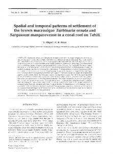
from 38 stations sampled from 1919 to 1994 (1 observation yr-l). These species were selected because they are among the more abundant species along the Skagerrak coast (and thus present high frequencies in the survey data) and have high commercial value. The 38 stations were selected because the time series from these were complete or near complete over the 1919 to 1994 period (Table 1). The distance between the most distant stations is about 210 km. The stations are classified into 10 different regions (Fig. 1, Table l), each region containing between 2 and 8 stations. Torvefjord, Bufjord, Flerdevigen and Sterlefjord correspond to coastal areas drectly open to the Skagerrak Sea. Hervdg and Soppekilen are defined as enclosed coastal areas. Topdalfjord, Sandnesfjord, Serndelefjord and Kilsfjord represent typical fjords within which the stations located at the entrance of the fjord are more exposed than the stations inside the fjord. The Norwegian Skagerrak gadoids. Cod populations from the Norwegian Skagerrak coast are non-migratory and grow faster than the northern Atlantic populations (e.g. the Arcto-Norwegian cod) but slower than those from the North Sea (Daan 1974, Garrod 1977, Fig. 1. Norwegian Skagerrak coast (northwest Europe). Detailed map shows Gjersater 1990, Danielssen & GjOszter the locations of the 38 studied stations. The 38 times series (stations) were lgg4,Gjerszter et lgg6). obtained from an extensive research survey, the 'Fl~devigendata set', and occurs at an earlier age than for the were sampled from 1919 to 1994. For each area or fjord (10 in all), the number of stations is given in parentheses. Five series of cod are shown as examples North Sea and the northern populations, (raw data) at around 2 to 3 yr (Gjersater et al. 1996). Little is known about the stock structure of pollack and whiting from the Norwegian Skagerrak coast. Pollack is caught totava 1990). Such a transformation is furthermore biogether with cod in the coastal fisheries, but the landlogically reasonable since population dynamics are ings are small (Anonymous 1993). Nothing is actually largely governed by multiplicative processes (Wilknown about the feeding ground of the whiting popliamson 1972). Before the log-transformation, a conulation. Only juveniles of the 0-group are usually stant of unity, i.e. the lowest possible catch value, was caught in shallow waters and in the fjords. Older added due to the occurrence of zeros. During the Second World War (1940 to 1944), the fishes seem to migrate into deeper water. Most fisheries are linked primarily to cod and secondarily to sampling was interrupted at all the stations, except at pollack. No fishery is specifically directed towards the 2 stations from Flerdevigen (Table 1). For the precoastal whiting. war period, 29 time series (i.e. stations) of the 38 are complete and 12 contain 1 or 2 missing values. In the post-war period, 35 time series are complete and 3 NUMERICAL ANALYSES have 1 to 3 missing values (Table 1). These short gaps were interpolated using the ZET method (Zagoruiko & The data were log-transformed (using the natural Yolkina 1982). Interpolating the 5 consecutive war logarithm) to stabilise the variance (e.g. Sen & Srivasyears (1940 to 1944) is not feasible because of the
212
Mar Ecol Prog Ser 155: 209-222, 1997
extensive variability inherent in these biological time series and insufficient knowledge of the biological processes. Each species was hence represented by a matrix of 38 series of log-abundance across 71 years (the 1919 to 1994 period less the 1940 to 1944 war years). The analyses were conducted for each species separately. Correlation analysis, principal component analysis (PCA), Mantel statistic and Mann-Whitney test (see below) were performed on the matrices of 38 stations by 71 years. Spectral analysis, which requires temporal contiguity, was applied to a restricted data set, only covering the 1945 to 1994 period (i.e. matrices of 38 stations by 50 years). Spatial patterns and correlation. For each species, we computed the average of the log-abundances over the 71 years. We thus obtained the 'average spatial pattern' of each species, which was represented by a vector of 38 values. The purpose of this was to detect locations of high and low abundance for each species and to permit a quantification of CO-occurrence between species. Comparisons between the 'average spatial patterns' of the 3 species were made using the Pearson correlation coefficient. Because of spatial autocorrelation in the 3 'average spatial patterns', the assumption of independence, which is required in the usual test of correlation, was violated (see e.g. Legendre 1993). We therefore applied a spatially correlated error model to correct for this (using Spacestat ver. 1.80; Anselin 1995), in which spatial correlation was taken to be inversely proportional to the squared distance between the stations. Five of the 10 regions have both sheltered stations inside fjords and exposed stations at the entrance of fjords (Table 1). To test for consistent differences in abundance between sheltered and exposed stations, we performed simple Mann-Whitney tests. The Mann-Whitney test between 2 samples (here a sample being a series of 71 years) is the non-parametric analogue of the paired t-test between 2 samples, but is both more appropriate and powerful for non-normal distributions (Zar 1984). Thus, we performed 1 MannIVhitney test for each species at each of the 5 regions (15 tests in total). Because of both spatial and temporal autocorrelation in the data, the assumption of independence was also violated. We did not, however, see any statistical remedy for this. We resorted therefore to interpreting the level of significance (fixed at 5%) with care. We stress, however, that the level of significance was not very critical to the analysis, since our purpose was to check for a consistent pattern over the 5 fjords. The Mantel test (Mantel 1967) was also performed to investigate the consistency of the spatial structure in the data of each species. In our application of this test,
the null hypothesis H, was: correlations between the 38 time series of a given species are independent of the geographical locations of these time series. This test is analogous to the linear correlation between 2 vectors of distances (Smouse et al. 1986). To perform it, we had to calculate 3 matrices of biological distances (1 for each species) and a matrix of geographical distances. The matrix of biological distances corresponds to the distances between the 38 time series of a species (measured by l minus the pairwise correlation coefficients between the 38 time series). The matrix of geographical distances corresponds to the distances in kilometres between the 38 stations. The test was performed for each species as the correlation between the matrix of biological and geographical distances. Due to interdependence between distances, a permutation test was used to evaluate the level of significance (Legendre & Fortin 1989). Repeatedly permuting the geographical matrix at random, followed by recomputation of the correlation, produces an empirical null distribution against which the actual value of correlation was tested (10 000 permutations were made for each Mantel test). Temporal patterns and correlation. To identify the main temporal patterns of each species across all the stations, we used PCA. PCA summarises in a few dimensions (i.e. the principal axes) most of the variability of a large number of descriptors and provides the variance explained by each principal axis-(see e.g. Legendre & Legendre 1984). Here, a PCA was performed for each species on the covariance matrices of the log-abundances, using the stations as the descriptors. The first axis of each PCA corresponded to the dominant temporal pattern of each species shared by all the stations, and is described by the row-scores of the first axis of the PCA (i.e. a series of 71 values for each species). The first axis was strongly related to the average of the log-abundances over all the stations, but provided, in addition, the percentage of variance associated with this average. We also looked at the second axis of each PCA, that displayed the secondary dominant temporal pattern for the 3 species across all the stations. The PCA also gave an indcation about the spatial variability, since the percentage of variance explained by the first 3 principal axes may be related to the level of spatial homogeneity (the greater the variance explained by the 3 first axes, the lower the differences between stations). Comparisons between the dominant temporal patterns of the 3 species (i.e. the row scores of the first axis of each PCA) were made using the Pearson correlation coefficient. Because of temporal autocorrelation in these time series, the assumption of independence was violated (see e.g. Ostrom 1987). To remedy this, we
Fromentin et al.: Spatio-temporal dynamics of three gadoid species
applied a temporally correlated error model (using PROC. AUTOREG.; SAS Institute 1990).As autocorrelation only occurs at lag 1, a first-order autoregressive model was assumed for the error. In order to distinguish correlation resulting from similar long-term trends between species from synchronous year-to-year fluctuations, correlation coefficients were also computed between the first-order differenced series (see 'Patterns of periodicity'). As these series did not display any autocorrelation, the level of significance was estimated as usual. Patterns of periodicity. All the above analyses refer to the time domain. In order to extract the patterns of periodicity, we analysed the series in the frequency domain. Spectral analyses were performed on the 38 series of each species for the 1945 to 1994 period. As most of the series displayed long-term trends and as the data were non-seasonal (1 point per year), the series were made stationary by computing the firstorder difference (Chatfield 1989); specifically, denoting x(t) the logarithm of the abundance at time t, the first-order difference of the series is: y(t) = x ( t +l )- x(t); y(t) corresponds, in a loose sense, to the interannual population growth. Applying first-order differencing led to emphasis of short-term oscillation (lower than 10 yr). We chose this because the longer periods, i.e. trends, were investigated within the PCAs on log-abundance (see 'Temporal patterns and correlation'). The spectral decomposition transforms each time series into a sum of sine and cosine functions of different period lengths. The raw periodogram is the usual way to summarise this decomposition. However, it is a poor statistical descriptor of the spectral density, since it is not consistent (Priestley 1981). We therefore used a Parzen smoothing window, with a width of 5, as recommended for short time series (Priestley 1981). In order to test for significance of the periodic fluctuations in the differenced series, a permutation test was used. Repeatedly permuting each series at random, followed by recomputation of the first-order difference and spectral analysis, produces an empirical null distribution against which the actual periodic fluctuation was tested (5000 permutations were made for each series). After the spectral decomposition, each species was represented by 38 series of spectral densities (1 per station). A PCA was then performed for each species on the matrix of spectral densities, to identify the dominant frequencies of each species across the 38 stations. Mapping of the row-scores, using the computer program ADE (Chessel & Deledec 1992), was performed to describe the spatial distribution of these main frequencies (see Bjernstad et al. 1996 for a detailed discussion).
213
RESULTS Spatial patterns and correlation The 'average spatial patterns' indicated relatively high differences in abundance from one location to another (Fig. 2), especially for whiting. The differences between the highest and the lowest log-transformed values were 3.5,2.3and 4.8 for cod, pollack and whiting respectively. High abundances were generally found at different locations for the 3 species. These were: Topdalfjord, Bufjord, Fledevigen and some stations of Sandnesfjord and Kilsfjord (areas 2, 4, 5, 6 and 9) for cod (Fig. 2a);
High abundance
-
Pollcrck ( b )
Whiting ( c )
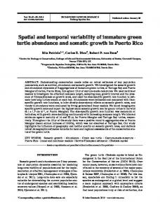
Fig. 2. Mapping of the 'average spatial patterns' of each species, i.e. the average of the log-abundances over the 71 years at each station, for (a) cod, (b) pollack and (c) whiting. Each series is centred around its mean (calculated over the 38 stations). ( 0 )Stations having a log-abundance higher than the mean (i.e. positive value); ( 0 )stations having a log-abundance lower than the mean (i.e. negative value). The size of the symbols is proportional to the absolute value at each station
214
Mar Ecol Prog Ser 155: 209-222, 1997
Table 2. Pearson correlation coefficients between the 'average spatial patterns' of the 3 species. Because of the presence of spatial autocorrelation in the series, a spatially correlated error model was performed using Spacestat ver. 1.80 (Anselin 19951 to obtain an unbiased estimate of the level of sianifi., cance of each correlation coefficient (spatial weights being inversely proportional to the squared distance between the stations). Bold type indicates significance
l Pollack Whiting
Cod
Pollack
-0.06 (p > 0.05) 0.59 (p < 0.01)
-0.26 (p > 0.05)
I
Torvefjord and at the entrance stations of Hsvdg and S~ndelefjord(areas 1, 3 and 7) for pollack (Fig. 2b); and some stations of Topdalfjord, Fladevigen, Sandnesfjord, S~ndelefjordand Kilsfjord (areas 2, 5, 6, 7 and 9) for whiting (Fig. 2c). Low values were recorded for cod and whiting at H ~ v i g Soppekilen , and at the entrance stations of S~ndelefjord(areas 3, 7 and 10), whereas low values of pollack were mainly situated at Kilsfjord and Soppekilen and at the inner stations of Topdalford, H0vAg and Sandnesfjord (areas 2, 3, 6, 9 and 10). The correlation coefficients between the 3 'average spatial patterns' corroborate the previous observations (Table 2): only the correlation between cod and whiting was high and significant. This suggests that these 2 species have similar habitats, being different from that of pollack. The similarity between cod and whiting was also apparent from the results of the Mann-Whitney tests, that compared abundances inside and at the entrance of a fjord. In 100% of the cases (i.e. in the 5 studied fjords), cod and whiting showed significantly higher abundance for stations inside the fjord. In contrast, pollack showed significantly higher abundance at the entrance stations in 4 of the 5 fjords, and no significant differences in the remaining case. Thus, a clear contrast appeared between pollack on one hand, for which the preferred habitat appeared to be in more open waters, and cod and whiting on the other, for which the preferred habitat seemed to be in the sheltered waters. These results suggest high spatial variability. Thus, it must be determined whether the temporal fluctuations of the juveniles of these 3 species are spatially structured at all. The Mantel tests clearly indicate that there is a spatial structure in the temporal variations of the 3 species, and that differences in temporal patterns from one location to another partially depend on geographical distance between locations. The Mantel correlation coefficients between fish temporal dynamics and geographical locations were 0.25, 0.18 and 0.24 for cod, pollack and whiting respectively, being signifi-
cant at the 0.1 % level for cod and whitinu., and at the 1 level for pollack. It appears that the spatial strutture is more pronounced for cod and whiting than for pollack.
Temporal patterns and correlation The first 3 axes of the PCA on log-transformed data encompassed 67% of the total variance for pollack, 52 % for cod and only 42 % for whiting. The first axis, corresponding to the dominant temporal pattern, accounted for a varying percentage of the total variance in the 3 species (Fig. 3a, b, c): about 56 % for pollack, 36 % for cod and only 23 % for whiting. The dominant temporal patterns mainly reflected the longterm trends and occurred in 95% of the stations for pollack, 78% of the stations for cod, and 31 % of the stations for whiting. The pollack was clearly most synchronous across the studied area. For cod and pollack, the trends were quite similar: a decline from the 1919 to 1939, followed by a n increase marked by the outburst from 1955 to 1965 (stronger for cod) and a second decline during the last 30 yr (with a second short period of high abundance around 1972 to 1975). It appears that the second decline, which was more conspicuous for pollack, began somewhat earlier for pollack than for cod. The year-to-year fluctuations were furthermore relatively synchronous between these 2 species. Correlation analysis confirms that cod and pollack had similar trends as well as similar yearto-year fluctuations (Table 3). For whiting, the trend was characterised by a long and regular increase from 1919 to the middle of the 1960s and a subsequent decline during the most recent years (Fig. 3c). Correlation coefficients between the Table 3. Pearson correlation coefficients between the dominant temporal patterns of the 3 species (i.e. the row scores of the first axis of the PCAs on the log-abundances). Due to autocorrelation in these series, a temporally correlated error model (using PROC AUTOREG; SAS Institute 1990) was used to test the level of significance (a first-order autoregressive model was assumed for the error). Correlation coefficients were also performed on the first-order differenced series (shown in italic), to distinguish correlations resulting from similar long-term trends between species from synchronous year-to-year fluctuations between species. Bold type indicates significance
Pollack Whiting
Cod
Pollack
0.57 (p < 0.01) 0.41 ( p 0.01) 0.16 (p > 0.05) 0.28 ( p c 0.05)
-0.12 (p > 0.05) 0.19 (p > 0.05)
Fromentin et al.: Spatio-temporal dynamics of three gadoid species
Dominant temporal pattern (axis 1)
1920
1940
1960
Secondary dominant temporal pattern (axis 2)
1980
1920
1940
years
g
-5
10
In
0
U
V)
0
-
O
0
-10 1920
a
1940
1960
5
5
E0
U
S O
5 LI
1980
Y
0
m 0
a
-5 1920
1940
5 LI
-g
10
o 1960
1980
m C
$ 0
1980
years
-
5
01
.-.-.-
1940
V)
E0
f -10 1920
1960
years
E0 0
1980
V)
years V)
1960
years
V)
5 LI
215
S 7 7
U
m C ...-
5 K
-5 1920
L
3 1940
1960
1980
years
Fig. 3. Principal component analysis (PCA) computed for each species on the covariance matrix of the log-abundances, using stations as descriptors. Panels correspond to the row scores of axis 1 (the dominant temporal pattern) and of axis 2 (the secondary dominant temporal pattern) of the PCA, for (a, d) cod, (b,e)pollack and (c, f ) whiting. The percentage of variance associated with each axis is given in parentheses. The plots take into account the gap corresponding to the missing values of the World War years (1940 to 1944). The periods 1919 to 1939 and 1945 to 1994 were subsequently fitted separately with a third-order polynomial function to highlight the trends. Dotted line: mean of the series (calculated over the 7 1 years)
dominant temporal patterns of the 3 species confirm that the pattern of whiting was very different from those of cod and pollack (Table 3). Nevertheless, correlation coefficients between the differenced series of these dominant temporal patterns showed that the year-to-year fluctuations of the whiting were significantly correlated with those of cod, but not with those of pollack. For cod, the second axis (i.e. the secondary dominant temporal pattern) displayed a clear downward trend until 1960 followed by an upward trend until the middle of the 1980s (Fig. 3d). This secondary temporal pattern was found in only a few stations (mainly in the northeast areas: Serndelefjord and Kilsfjord),where the dominant pattern was not observed. For pollack, the second axis accounted for a very small percentage of the total variance (10 times lower than the first axis). This axis corresponds to a strong drop in abundance during the 1930s (Fig. 3e), and it was found mainly at some of the stations in Hervbg, Kilsfjord and Soppekilen. For whiting, the second axis displayed high abundances from 1919 to 1950, a regular decline during the following 30 yr and a slight increase in the last years. As for cod, this secondary pattern occurred in
stations (mainly in the northeast areas: Sandnesfjord and Kilsfjord) where the dominant pattern was not observed. The results of the PCA stress the presence of pronounced regional differences. This was firstly shown by the low percentages of variance explained by the first 3 axes (especially for whiting). Secondly, the northeast stations displayed, for cod and whiting, a very different temporal pattern from the dominant one, which mainly occurred for these 2 species in southwest stations. The dominant pattern was, however, much more pronounced for pollack than for cod and whiting. Furthermore, it appears that the dominant patterns of cod and pollack were both different from that of whiting. Nevertheless, there has been a clear drop in the abundance of the 3 species since the 1970s, but less pronounced for whiting than for the 2 other species.
Patterns of periodicity The permutation tests for the spectral densities on differenced series revealed significant (5% level) short-term periodicity (2 to 5 yr) in 50, 34 and 68% of
Mar Ecol Prog Ser 155: 209-222, 1997
216
the stations and significant longer periodicity (> 5 yr) in 11, 26 and 8 % for cod, pollack and whiting respectively (in the other stations no special periodicity was found). Hence, all species showed evidence of highfrequency variations, especially cod and whiting for which the long-term trends were less pronounced (see 'Temporal pattern and correlation'). To summarise the patterns of periodicity, a PCA was performed on the 38 series of spectral densities of each species. The first axis, which detects for each species the dominant pattern of periodicity across the 38 stations, encompassed 69, 56 and 50% of the total variance for cod, pollack and whiting, respectively (the first 3 axes captured 92, 92, and 87 % of the total variance). This indicates that the first axis captured the bulk of the total variation in spectral densities. For the 3 species, the dominant frequency identified by the first axis of the PCA was around 2 to 2.5 yr (Fig. 4a, b, c). Series (stations) that did not display this main cycle exhibited no special periodicity and spectra resembling those expected for a series of random num-
Axis 2
Axis 1
-
h
g -5 E
W
v
... .
0
a,
a
*0
- . .. . . . . .
0
0
v
v
.
0.5
0
0.5
0
a,
v
.
bers (Fig. 4a, b, c). The second and third axes modulated the dominant periodic behaviour in series exhibiting a clear maximum at 2 to 2.5 yr. The second axis distinguished, for the 3 species, stations that exhibited a purely 2 yr fluctuation from those that showed a 2.3 to 3 yr periodicity (Fig. 4d, e , f). The third axis distinguished, for each species, stations with a 2 to 2.5 yr period from those having a 3.5 yr periodicity (Fig. 4g, h, i). Hence, the dominant patterns of periodicity in the differenced time series were similar between species. Fig. 5 depicts the spatial distribution of the row scores of axis 1 (axes 2 and 3 are not shown as they account for only a small part of the total variance).The periodic patterns show consistent spatial variations that vary between the 3 species. These patterns result from differences occurring at a mesoscale (differences between fjords) and at a local scale (differences within a fjord). For cod, the pattern of periodicity appears strongly related to the level of abundance (Fig. 6a); the higher the average abundance in a station, the stronger is the evidence of a 2 to 2.5 yr cycle. Areas or fjords that exhibited low abundance Axis 3 (Hevbg and some stations of Sendelefjord) did not display periodic fluctuati0.s (open squares in Fig. 5a), whereas areas with high abundance v 8 (Topdalfjord, Bufjord, Fledevigen) . . showed clear evidence of a 2 to 2.5 yr 0.5 cycle (black circles in Fig. 5a).The spatial pattern was consistent at the local scale. The stations situated inside the fjords or areas displayed clearer 2 to ..
-E 2
m
m
0
0
.
0 W
a
0
0.5
0.5
..
. - -
a
0
W
. . 5m
Sa
0.5
0
. . W
v
a, .. -
0
c 3
0.5
frequency
c 0
0.5
frequency
0'5
0
frequency
Fig. 4. Spectral densities, using a Parzen window (width 5), were estimated from the 38 first differenced time series of each species. For each species, a PCA was computed using spectral densities as descriptors. The first 3 axes encompassed 92,92 and 87 % of the total variance for cod, pollack and whiting respectively. For the 3 species, axis 1 of the PCAs distinguishes stations with a-2 to 2.5 yr cycle (solid line) and stations with no special periodicity (dotted h e ) . The second and third axes modulate the dominant periodic behaviour in series exhibiting a clear maximum at 2 to 2.5 yr. Axis 2 discriminates stations exhibiting a purely 2 yr fluctuation (solid line) with those showing a 2.3 to 3 yr periodicity (dotted line); and axis 3 distinguish stations with a 2 to 2.5 yr period (solid line) and those having a 3.5 yr periodicity (dotted line). Dominant frequencies detected by the PCA are shown for (a, d , g) cod, (b, e, h) pollack and (c, f , i) whiting
2.5 yr cycles than those situated at the entrance or outside of the fjords. This was especially obvious for the Topdalfjord, Fledevigen and Sandnesfjord areas (Fig. 5a). For pollack, a similar relationship between the level of abundance and the periodicity was apparent (Fig. 6b). Areas with high abundance (Torvefjord, Sendelefjord), showed clear 2 to 2.5 yr fluctuation (black circles in Fig. 5b). In contrast, areas with low abundance (some stations of Topdalfjord, Hevbg, Sandnesfjord and Soppekilen) generally did not display any clear periodicity (open squares in Fig. 5b). Differences between stations located inside and at the entrance of fjords also occurred, but in contrast to cod, the sheltered stations generally displayed less clear cycle than the exposed stations, as seen at Topdalfjord, Hevbg
Fromentin et al.: Spatio-temporal dynamics of three gadoid species
217
10
+
(a):cod 3.9
Sandnesfjor
Pollack (b)
1
Torvefjord
(c):whiting
+
r2=0.03
l
Whiting ( c )
0
1
2
3
4
log-abundance
Fig. 5. Mapping of the first row scores of the PCAs computed on the spectral densities; (a) cod), (b) pollack and (c) whiting. ( 0 )Stations showing a clear 2 to 2.5 yr cycle; ( 0 )stations exhibiting no periodic fluctuations. The size of the symbols is proportional to the absolute value of the score and thus to the importance of the periodicity
and Serndelefjord (Fig. 5b). This reflected the shift in areas of high abundance, cod being more abundant inside fjords while pollack was more abundant at the entrance of the fjords (above). For whiting, the spectral pattern is more difficult to interpret and the simple linear relationship between the level of abundance and the periodicity vanishes (Fig. 6c). Areas with high abundance displayed either a clear 2 to 2.5 yr fluctuation (black circles in Topdalfjord and Sandnesfjord; Fig. 5c) or no periodicity (open squares in the stations at Flerdevigen, Serndelefjord and Kilsfjord; Fig. 5c). However, areas with low abundance (Soppekilen and some stations of Hervbg and Serndelefjord)did not display any periodic fluctua-
Fig. 6. Scatterplots of the average log-abundances in the 38 stations (calculated over the 71 years) vs the first row scores of the PCA computed on the spectral densities (i.e. the magnitude of the 2 to 2.5 yr oscillation); (a) cod, (b) pollack, (c) whiting. The relationships are estimated by simple linear regressions, r2 being the coefficients of determination
tions. Periodicity is generally more apparent at the typical fjords (e.g. Topdalfjord, Sandnesfjord) and at stations inside enclosed coastal areas (e.g. Hervbg) and less manifest at the more exposed coastal areas (e.g. Flerdevigen and Bufjord) or at the stations at the entrance of the enclosed coastal areas (e.g. Hervbg). Despite important differences between species at the mesoscale, there was a relationship between the level of abundance and the evidence of the 2 to 2.5 yr oscillation (Fig. 6), especially for cod and pollack. Furthermore, spatial patterns of cod and whiting were characterised by some similarities: they generally showed clearer periodic fluctuations in the sheltered stations. This was clearly different from that of pollack, which displayed clearer periodic fluctuations in the more exposed areas.
Mar Ecol Prog Ser 155: 209-222, 1997
218
DISCUSSION Spatial variations in temporal dynamics A conspicuous result that emerged from the various analyses was the presence of a high spatial variability. Firstly, at a mesoscale: some areas or fjords were characterised by high abundance for a given species (e.g. Topalfjord, Bufjord and Flerdevigen for cod) whereas others locations displayed consistently low abundance (e.g. Hervbg for cod). Secondly, at a local scale: the species were not regularly distributed at the scale of the fjord; significant differences occurred between sheltered and exposed stations. The spatial variability was also reflected in the low percentages explained by the first 3 axes of the PCA computed on log-abundance. The spatial heterogeneity was most conspicuous for cod and whiting, for which the second PCA axes showed that northeast stations displayed a very different temporal pattern from that of axis 1, which were mainly recorded in southwest stations. Analyses of periodic fluctuations further highlighted spatial variability that resulted from differences occurring at a mesoscale and at a local scale. At mesoscale, some areas or fjords (varying among the 3 species) displayed evidence of a 2 to 2.5 yr cycle, whereas other areas &d not. At local scale, cod and whiting generally exhibit clear cycles at sheltered stations, whereas pollack showed clearer oscillations at stations located at the entrance of fjords. In summary, all analyses demonstrated that abundance of the 0-groups of these 3 gadoids from the Norwegian Skagerrak coast were highly variable in space and time. However, Mantel tests, the Mann-Whitney tests and the mapping of the results indicated that this variability was strongly structured in space.
Comparison of spatial patterns between species The extent of the spatial variability appeared species-specific. Whiting exhibited the highest variability in space, whereas pollack exhibited the lowest. For the former species, the variance around the yearly average (based on all the stations) was much higher than for cod and pollack. This was particularly obvious from the PCAs on log-abundance. For pollack, the first axis explained more than half of the temporaI fluctuations (with 95% of the stations exhibiting such a pattern). The dominant temporal pattern for whiting, in contrast, only occurred at 31 % of the stations and only explained 23 % of the total variance. Cod was intermediate between these 2. The Mann-Whitney tests indicated a clear contrast between cod and whiting on one hand and pollack on
the other. The former species were more abundant inside fjords whereas the latter was more abundant at the entrance of fjords. This is consistent with other studies from a smaller area of the Norwegian Skagerrak coast (Gjersaeter & Danielssen 1990) and from the Norwegian west coast (Goder et al. 1989), which also showed that cod and whiting were generally located inshore and absent from the more exposed areas, whereas pollack settled at more exposed locations. Species that were more abundant inside fjords or in the protected areas (cod and whiting) exhibited greater spatial variability than the species that were more abundant at the entrance of fjords (pollack).The Mantel tests corroborated this, since the spatial patterns of cod and whiting were more spatially structured than that of the pollack. This difference probably results from the division of the inner fjords into many, partly isolated habitats, while the outer coastal areas are more homogeneous. Relatively enclosed fjord populations might also show greater variations because they are more dependent on local wind and current changes than more exposed populations (Aksnes et al. 1989).
The 2 to 2.5 yr oscillation Our analyses document an oscillatory component in the 3 gadoid species that was dominated by frequencies around 2 to 2.5 yr. This periodic component was closely related to the level of abundance and both were strongly spatially structured. This leads us to postulate that there are optimal habitats along the Norwegian Skagerrak coast (sheltered areas for cod and whiting and more exposed areas for pollack) where level of abundance and periodicity of each fish population are more apparent, and non-optimal habitats where level of abundance and periodicity are less manifest. The lack of periodicity in some stations may reflect 'source-sink' dynamics (e.g. Pulliam 1988, Stenseth & Lidicker 1992). Individual fishes may persist in 'sink' habitats (non-optimal ones), where demographic processes are insufficient to maintain the population, because of immigration from the more productive 'source' habitats nearby (optimal ones). Periodicity in the fluctuations of age-structured populations can depend on the manifestation of competition between cohorts (e.g. Caley et al. 1996),with periods equal to the generation time or 2 times the generation time (depending of the kind of the competition involved; Gurney & Nisbet 1985). For the Norwegian Skagerrak cod, maturation (and thus generation time) occurs at an age of 2 to 3 yr (the 2 and 3 yr classes constitute 50 and 25% of the spawning stock respectively; Gjersceter et al. 1996).Competition between different cohorts of this population is highly probable,
Fromentin et al.: Spatio-temporal dynamics of three gadoid species
since (1) N. C. Stenseth, 0. N. Bj~rnstad,W. Falck, J . M. Fromentin, J . Gjrasceter & J. Gray (unpubl.) have demonstrated significant density-dependence in recruitment of the Norwegian Skagerrak cod; (2) cannibalism between stages has been demonstrated for the southern Norwegian cod stock (Hop et al. 1992); and (3) competition for food and space between the older classes and the 0-group is likely to occur in these fjords where the number of habitats is limited (T. Johannessen pers. obs., based on diving observations). Competition for food and space is furthermore consistent with the presence of optimal and non-optimal habitats. Thus, competition between different stages might explain the 2 to 2.5 yr periodicity in the Norwegian Skagerrak cod populations. Such an oscillatory component is likely to be longer for other cod stocks, for which maturation occurs at around 5 to 7 yr (Cushing 1982). The 3 species of gadoids have a similar life cycle. The conclusions regarding the cod may therefore be extended to understand the 2 to 2.5 yr cycle of pollack and whiting as well. Consequently, we hypothesise that the dominant 2 to 2.5 yr fluctuation results from biotic processes such as density-dependent survival due to competition for food and space and cannibalism between stages (see Myers & Cadigan 1993 for a related discussion on density-dependent juvenile mortality in marine demersal fish).
Interactions in time and space between species The correlation analyses document that the 3 species were related in either space or time. Cod and whiting exhibited similar spatial patterns in abundance, which were likely to be due to similar propensity for sheltered habitats. These 2 species showed divergent long-term trends but their year-to-year fluctuations had similarities. In contrast, cod and pollack displayed highly similar trends and year-to-year fluctuations, while they showed different habitat preferences at a meso- and at a local scale. Pollack and whiting did not show.any relationship in abundance in space or in time. Under the hypothesis of limited space and food resources, there may be spatial structuring due to interspecific competition. It is however difficult to speculate on this, as the feeding ground of whiting is unknown.
Long-term trends It is likely that extrinsic forces induce the long-term trends in these populations. Four main reasons led to this conjecture: (1) intrinsic processes seemed to be related to short-term fluctuations (i.e. the 2 to 2.5 yr cycle); (2) despite local- and mesoscale habitat differ-
219
ences between cod and pollack, these 2 species displayed highly similar year-to-year fluctuations and long-term trends; (3) all 3 species have shown a strong decline since the 1970s; (4) the literature often refers to external influences to explain trends in fish populat i o n ~either , through overfishing (e.g. Garrod & Shulmacher 1994, Myers et al. 1996),through variations in food availability (e.g. Skreslet 1989, Cushing 1995, Sundby 1995), or through climatic and hydrographic changes (e.g. Koslow et al. 1987, Cury & Roy 1989, Ellersten et al. 1989, Dickson & Brander 1993, Mann 1993, Conover et al. 1995, Ottersen & Sundby 1995).
Long-term trends versus environmental changes and overfishing Two important environmental changes have taken place along the Norwegian Skagerrak coast during the period in which the recent decline of these 3 fish population~has occurred: (1) a severe decline of Calanus finmarchicus (Fromentin & Planque 1996, Planque & Fromentin 1996), from which the nauplii and the first stages of copepodites constitute the major resource of fish larvae (Ellersten et al. 1981, Skreslet 1989, Thorisson 1989, Brander & Hurley 1992);and (2) eutrophication and subsequent decline in the oxygen concentrations of the Norwegian Skagerrak coastal waters (Aure et al. 1996, Johannessen & Dahl 1996). The presence of a strong decline during the 1920s and the 1930s in cod and pollack series points also to the possibility of an environmental impact. Effects of meteorological and hydrological conditions on the temporal dynamics of early stages of fjord populations have already been shown. For instance, Johannessen & Tveite (1989) suggested that water mass stability might be important during March and April for the magnitude of the year classes of the Norwegian Skagerrak cod. Aksnes et al. (1989) concluded that the level of the biomass and the stability of mesozooplankton predators, as early stages of cod, may depend on the strength and variability of the transport processes. Lindahl & Hernroth (1988) also pointed out the importance of advective processes in regulating zooplankton biomass, the primary source of food for fish larvae. Besides these relationships between meteorological factors and fish, it appears that the bottom flora coverage over the Norwegian Skagerrak coast (mainly Zostera marina) has greatly fluctuated during this century. Z. marina declined abruptly and severely during the 1930s due to a seagrass illness, then recovered from 1945 to 1965 and has displayed a slight decrease since then (Johannessen & Sollie 1994).These fluctuations, which fitted the long-term trends of cod and pollack until the mid-1960s, could lead to important con-
220
Mar Ecol Prog Ser
sequences for juveniles and adult fish, which mainly feed on the bottom fauna. Little is known about the fishing effort on these coastal populations, but it is likely that the fishing effort has been fairly constant along the Norwegian Skagerrak coast since the beginning of the century. The recent decline of whiting is less pronounced than for cod and pollack, for which the impact of coastal fishing is more conspicuous. Hence, we cannot dismiss 'recruitment overfishing' (i.e. overfishing that would affect recruitment and not only the parent stocks, see Myers & Barrowman 1996) as a cause of the recent decline. Nevertheless, the overfishing hypothesis (with constant or increasing effort) cannot entirely explain the origin(s) of long-term trends, in particular why cod and pollack populations strongly declined during the 1930s and then increased to reach high abundance from 1955 to 1965. Further work is needed to determine the origin(s) of these long-term trends. The hypotheses developed above must be further tested. Furthermore, the amplitude of the hydrological and climatic changes in the Skagerrak area has also to be studied, as well as the impact of global events, such as the North Atlantic Oscillation (Hurrell 1995).
Conclusion The present study of the 0-group of 3 gadoid species from the Norwegian Skagerrak coast leads to 5 main conclusions: (1) there is great spatial variability in the abundance as well as in the patterns of year-to-year fluctuations; this variability is strongly structured in space and occurs at a meso- and a local scale; (2) the degree of spatial variability is species-specific; cod and whiting, which are more abundant in the sheltered areas, exhibit higher spatial variations than pollack, which is more abundant in more exposed areas; (3) temporal dynamics of these populations appear more regular in areas of high abundance (in optimal habitats); (4) the 3 species exhibit periodic fluctuations of 2 to 2.5 yr in their optimal habitats, which possibly results from intrinsic interactions in an age-structured population, such as density-dependent survival due to competition and cannibalism; and (5) the long-term trends account for a large part of the total temporal variability and are likely to be induced by extrinsic forces, such as environmental changes or anthropogenic influences. Acknowledgements. First of all, our appreciation goes to the late Rangvald Leversen and to Aadne SolLie for carrying out the sampling resulting in the 'Fledevigen data set'. Thanks are due to a DN-funded project for organizing the data into computer-readable format. Financial support from the
University of Oslo (through the 'Environmental Program' to N.C.S.) and from the MAST-program of the European Union (fellowship contracts to J.M.F.) made the reported analyses possible. We also thank the anonymous referees for their helpful and constructive comments.
LITERATURE CITED Aksnes DL, Aure J , Kaartvedt S, Magnesen T, Rickard J (1989) Significance of advection for the carrying capacities of fjord populations. Mar Ecol Prog Ser 50:263-274 Anonymous (1993) Forvaltning av fiskeriressurserne i Skagerrak og Kattegat. Nordiske Seminar- og Arbejdsrapporter 1933 (550):l-214 Anselin L (1995) Spacestat-a software program for the analysis of spatial data (Ver. 1.80). Regional Research Institute, West Virginia University, Morgantown Aure J , Danielssen D, Saetre R (1996) Assessment of eutrophication in Skagerrak coastal waters using oxygen consumption in fjordic basins. ICES J Mar Sci 53:589-595 Bailey KM, Houde ED (1989) Predation on eggs and larvae of marine fishes and the recruitment problem. Adv Mar Biol 26:l-83 Bjernstad ON, Champely S, Stenseth NC, Saitoh T (1996) Cyclicity and stability of grey-sided voles, Clethrinomys rufocanus of Hokkaido: evidence from spectral and Principal components analyses. Phil Trans R Soc Lond B 351: 867-875 Brander KM (1994) Patterns of distribution, spawning, and growth in North Atlantic cod: the utility of inter-regional comparisons. ICES Mar Sci Symp 198:406-413 Brander KM, Hurley PCF (1992) Distribution of early-stage Atlantic cod (Gadus morhua), haddock (Melanogrammus aeglefinus) and witch founder (Glyptocephalus cynoglossus) eggs on the Scotian Shelf: a reappraisal of evidence on the coupling of cod spawning and plankton production. Can J Fish Aquat Sci 38:1125-1134 Caley MJ, Carr MH, Hixon MA, Hughes TP, Jones GP, Menge BA (1996) Recruitment and the local dynamics of open marine populations. Annu Rev Ecol Syst 27:477-500 Chatfield C (1989) The analysis of times series: a n introduction. Chapman & Hall, London Chessel D, Deledec S (1992) ADE: Hypercarda stacks and programme library for the analysis of environmental data (Ver. 3.7). URA CNRS 1451, University of Lyon 1, Villeurbanne Conover RJ, Wilson S, Harding GCH, Vass WP (1995) Climate, copepods and cod: some thoughts on the long-range prospects for a sustainable northern cod fishery. Clim Res 5:69-82 Cook RM, Sinclair A, Stefansson G (1997) Potential collapse of the North Sea cod stocks. Nature 385:521-522 Cury P, Roy C (1989) Optimal environment window and pelagic fish recruitment success in upwelling areas. Can J Fish Aquat Sci 46:670-680 Cushing DH (1982) Climate and fisheries. Academic Press, London Cuslung DH (1995) The long-term relationship between zooplankton and fish. ICES J Mar Sci 52:611-626 Cushing DH, Dickson RR (1976) The biological response in the sea to climatic changes. Adv Mar Biol 14:l-122 Daan N (1974) Growth of the North Sea cod Gadus morhua. Neth J Sea Res 8:27-48 Danielssen DS, Gjesaeter J (1994)Release of 0-group cod (Gadus morhua L.) on the southern coast of Norway in the years 1986-89. Aquatcult Fish Manage 25(Suppll):129-142
Fromentin et al.: Spatio-temporal dynamics of three gadoid species
Dickson RR, Brander KM (1993) Effects of a changing windfield on cod stocks of the North Atlantic. Fish Oceanogr 2: 124-153 Ellertsen B, Possum P, Solemdal P, Sundby S (1989) Relation between temperature and survival of eggs and first-feeding of the northeast Arctic cod (Gadus morhua L.). Rapp PV Reun Cons Int Explor Mer 191:209-2 19 Ellertsen B, Solemdal P, Sundby S, Tilseth S, Westgird T, 0iestad V (1981) Feeding and vertical distribution of codlarvae in relation to availability of prey organisms. Rapp PV Reun Cons Int Explor Mer 178:317-319 Fortier L, Villeneuve A (1996) Cannibalism and predation of fish larvae by larvae of Atlantic mackerel, Scomber scombrus, trophodynamics and potential impact on recruitment. Fish Bull 94:268-281 Fromentin JM, Planque B (1996) Calanus and environment in the eastern North Atlantic. 11. Influence of the North Atlantic Oscillation on C. finmarchicus and C. helgolandicus. Mar Ecol Prog Ser 134:lll-118 Garrod DJ (1977) The North Atlantic cod. In: Gulland JA (ed) Fish populations dynamics. John Wiley & Sons, London, p 216-242 Garrod DJ, Schumacher A (1994) North Atlantic cod: a broad canvas. ICES Mar Sci Symp 198:59-76 Gjesaeter J (1990) Norwegian coastal Skagerrak cod. Report on the ICES study group of cod stock fluctuations. Appendix 111. ICES Comm Meet 1990/G50:155-170 Gjesaeter J , Danielssen DS (1990) Recruitment of cod, Gadus moihua L., whiting, Merlangius merlangus, and pollack, Pollachius pollachius, in the Riser area on the Norwegian ~ k a ~ e r r a k c o a 1946st 1985. Fledevigen ~ a ~ ~ o r t s e 1: rce 11-31 Gjesaeter J , Enersen K, Enersen SE (1996) Ressurser av torsk og andre fisk I fjorder p i den Norske Skagerrakkysten. Fisken og Havet 23: 1-28 Gedo OR, Gjesaeter J , Sunnani K, Dragesund 0 (1989)Spatial distribution of 0-group gadoids off mid-Norway. Rapp PV Reun Cons Int Explor Mer 191:273-280 Gurney WSC, Nisbet RM (1985) Fluctuation periodicity, generation separation, and the expression of larval competition. Theor Popul Biol28:150-180 Hjort J (1914) Fluctuations in the great fisheries of Northern Europe. Viewed in the light of biological research. Rapp PV Reun Cons Int Explor Mer 20: 1-228 Hop H, Gjesaeter J , Danielssen DS (1992) Seasonal feeding ecology of Atlantic cod (Gadus morhua L.) on the Norwegian Skagerrak coast. ICES J Mar Sci 49:453-461 Hurrell JW (1995) Decadal trends in the North Atlantic Oscillation: regional temperatures and precipitation. Science 269:676-679 Hutchings JA (1996) Spatial and temporal variation in the density of northern cod and a review of hypotheses for the stock's collapse. Can J Fish Aquat Sci 53:943-962 Johannessen T, Dahl E (1996) Declines in oxygen concentrations along the Norwegian Skagerrak coast, 1927-1993: a signal of ecosystem due to eutrophication? Limn01 Oceanogr 41:766-778 Johannessen T, Sollie A (1994) Overviking av gruntvannsfauna p i Skagerrakkysten. Fisken og Havet 10:l-91 Johannessen T, Tveite S (1989) Influence of various physical environmental factors on 0-group cod recruitment as modelled by partial least-squares regression. Rapp PV Reun Cons Int Explor Mer 191:311-318 Koslow JA, Thompson KR, Silvert W (1987) Recruitment to Northwest Atlantic cod (Gadus morhua) and haddock ( M e l a n o g r a m u s aeglefinus) stocks: influence of stock size and climate. Can J Fish Aquat Sci 44:26-39
221
Laevastu T (1993) Marine climate, weather and fisheries. Blackwell Scientific Publications, Oxford Legendre L, Legendre P (1984) Ecologie numerique. Tome 2: La structure des donnees ecologiques. Masson, Presse d e l'universite du Quebec, Paris Legendre P (1993) Spatial autocorrelation: trouble or new paradigm? Ecology 74:1659-1673 Legendre P, Fortin MJ (1989) Spatial pattern and ecological analysis. Vegetatio 80:107-138 Lindahl 0,Hernroth L (1988) Large-scale and long-term variations in the zooplankton community of Gullmar fjord, Sweden, in relation to advective processes. Mar Ecol Prog Ser 43:161-171 Mann KH (1993) Physical oceanography, food chains, and fish stocks. ICES J Mar Sci 50:105-119 Mantel N (1967) The detection of disease clustering and a generalized regression approach. Cancer Res 27: 209-220 May RC (1974) Larval mortality in marine fishes and the critical period concept. In: Blaxter JHS (ed) The early life history of fish. Springier-Verlag, New York, p 3-19 Myers RA, Barrowman NJ (1996) 1s fish recruitment related to spawner abundance? Fish Bull 94:707-724 Myers RA, Cadigan NG (1993) Density-dependent juvenile mortality in marine demersal fish. Can J Fish Aquat Sci 50: 1576-1590 Myers RA, Hutchings JA, Barrowman NJ (1996) Hypotheses for the decline of the cod in the North Atlantic. Mar Ecol Prog Ser 138:293-308 Myers RA, Mertz G, Barrowman NJ (1995) Spatial scales of variability in cod recruitment in North Atlantic. Can J Fish Aquat Sci 52:1849-1862 Ostrom CW (1987) Time series analysis: regression techniques. Sage Publications, Beverly Hills Ottersen G, Sundby S (1995) Effects of temperature, wind and spawning stock biomass on recruitment of Arcto-Norwegian cod. Fish Oceanogr 4:278-292 Planque B, Fromentin JM (1996) Calanus and environment in the eastern North Atlantic. I. Spatial and temporal patterns of Calanus finmarchicus and C. helgolandicus. Mar Ecol Prog Ser 134:lOl-109 Priestley MB (1981) Spectral analysis and times series. Academic Press, London Pulliam HR (1988) Sources, sinks, and population regulation. Am Nat 132552-661 SAS Institute (1990) SAS/ETS user guide, Version 6, 4th edn. SAS Institute, Cary, NC Sen A, Srivastava M (1990) Regression analysis: theory, methods and applications. Springer-Verlag, New York Skreslet S (1989) Spatial match and mismatch between larvae of cod (Gadus morhua L.) and their principal prey, nauplii of Calanus finmarchicus (Gunnerus).Rapp PV Reun Cons Int Explor Mer 191:258-263 Smouse PE, Long CJ, Sokal RR (1986) Multiple regression and correlations extensions of the Mantel test of matrix correspondence. Syst Zoo1 35:627-632 Southward AJ, Boalch GT, Maddock L (1988) Fluctuations in the herring and pilchard fisheries of Devon and Cornwall linked to change in climate since the 16th century. J Mar Biol Assoc UK 68:423-445 Stenseth NC, Lidicker WZJ (1992) Animal dispersal: small mammals as a model. Chapman & Hall, London Sundby S (1995) Wind climate and foraging of larval and juvenile Arcto-Norwegian cod (Gadus morhua). In: Beamish RJ (ed) Climate change and northern fish populations. Can Spec Pub1 Fish Aquat Sci 121:405-415 Thorisson K (1989) The food larvae and pelagic juveniles of
222
Mar Ecol Prog Ser 155: 209-222, 1997
cod (Gadus morhua) in the coastal waters west of Iceland. Rapp PV Reun Int Explor Mer 191:264-272 Tveite S (1971) Fluctuations in year-class strength of cod and pollack in southeastern Norwegian coastal waters during 1920-1969. FiskDir Skr Ser HavUnders 16:65-76 Williamson M (1972) The analysis of biological populations. Edward Arnold, London Wooster WS, Bailey KM (1989) Recruitment of marine fishes revisited. In: Beamish RJ, Farlane GA (eds) Effects of
ocean variability on recruitment and a n evaluation of parameters used in stock assessment models. Can Spec Pub1 Fish Aquat Sci 108:153-159 Zagoruiko NG, Yolkina VN (1982) Inference and data tables with missing values. In: Krishnaiah PR, Kanal LN (eds) Handbook of statistics, North Holland Publishing Compagny, Amsterdam, p 493-500 Zar J H (1984) Biostatistical analysis, 2nd edn. Prentice-Hall, London
This article was submitted to the editor
Manuscript received: October 8, 1996 Revised version accepted: June 10, 1997