Spatial representativeness of air quality monitoring sites Outcomes of the FAIRMODE/AQUILA intercomparison exercise Kracht O., Santiago J.-L., Martin F., Piersanti A., Cremona G., Righini G., Vitali L., Delaney K., Basu B., Ghosh B., Spangl W., Brendle C., Latikka J., Kousa A., Pärjälä E., Meretoja M., Malherbe L., Letinois L., Beauchamp M., Lenartz F., Hutsemekers V., Nguyen L., Hoogerbrugge R., Eneroth K., Silvergren S., Hooyberghs H., Viaene P., Maiheu B., Janssen S., Roet D. and Gerboles M.
2017
EUR 28987 EN
This publication is a Technical report by the Joint Research Centre (JRC), the European Commission’s science and knowledge service. It aims to provide evidence-based scientific support to the European policymaking process. The scientific output expressed does not imply a policy position of the European Commission. Neither the European Commission nor any person acting on behalf of the Commission is responsible for the use that might be made of this publication. Contact information Name: Oliver Kracht Address: European Commission, Joint Research Centre, Via E. Fermi, 21027 Ispra (VA), Italy Name: Michel Gerboles Address: European Commission, Joint Research Centre, Via E. Fermi, 21027 Ispra (VA), Italy Email:
[email protected] Tel.: +39 033-278-5652 JRC Science Hub https://ec.europa.eu/jrc JRC108791 EUR 28987 EN
PDF
ISBN 978-92-79-77218-4
ISSN 1831-9424
doi:10.2760/60611
Luxembourg: Publications Office of the European Union, 2017 © European Union, 2017 Reuse is authorised provided the source is acknowledged. The reuse policy of European Commission documents is regulated by Decision 2011/833/EU (OJ L 330, 14.12.2011, p. 39). For any use or reproduction of photos or other material that is not under the EU copyright, permission must be sought directly from the copyright holders. How to cite this report: Kracht O., Santiago J.-L., Martin F., Piersanti A., Cremona G., Righini G., Vitali L., Delaney K., Basu B., Ghosh B., Spangl W., Brendle C., Latikka J., Kousa A., Pärjälä E., Meretoja M., Malherbe L., Letinois L., Beauchamp M., Lenartz F., Hutsemekers V., Nguyen L., Hoogerbrugge R., Eneroth K., Silvergren S., Hooyberghs H., Viaene P., Maiheu B., Janssen S., Roet D. and Gerboles M., Spatial representativeness of air quality monitoring sites - Outcomes of the FAIRMODE/AQUILA intercomparison exercise, EUR 28987 EN, Publications Office of the European Union, Luxembourg, 2017, ISBN 978-92-79-77218-4, doi:10.2760/60611, JRC108791. All images © European Union 2017
Contents Acknowledgements .............................................................................................. 1 Summary ........................................................................................................... 2 1 Introduction ................................................................................................... 4 2 Content of the Shared Dataset .......................................................................... 6 2.1 Measurements of the automatic stations for the city of Antwerp and its regional area for the year 2012. ............................................................................ 6 2.2 Measurements of the ATMOSYS-campaign with passive samplers and mobile stations .................................................................................................. 6 2.3 Gridded model data ................................................................................. 6 2.4 Virtual monitoring sites ............................................................................ 6 2.5 Emission inventories ................................................................................ 7 2.6 Gridded population density for the great Antwerp area .................................. 7 2.7 Cadastre of building heights for the city of Antwerp ...................................... 7 2.8 CORINE land use/cover classification within the domain ................................ 7 2.9 Virtual station dataset .............................................................................. 7 2.10 PM10 data (speciation) .............................................................................. 8 2.11 Daily traffic ............................................................................................. 8 3 General Description and Characterisation of the Datasets ...................................... 9 4 Participating Teams ........................................................................................14 5 Spatial Representativeness Methods used by the Participants ...............................15 5.1 Brief methods descriptions .......................................................................15 5.1.1
CIEMAT ..........................................................................................15
5.1.2
ENEA .............................................................................................15
5.1.3
EPAIE ............................................................................................16
5.1.4
FEA-AT ...........................................................................................16
5.1.5
FI ..................................................................................................16
5.1.6
INERIS ...........................................................................................16
5.1.7
ISSEeP & AwAC ...............................................................................17
5.1.8
RIVM .............................................................................................17
5.1.9
SLB ...............................................................................................17
5.1.10 VMM ..............................................................................................18 6 Reporting of Data and Results ..........................................................................22 7 Quantitative Outcomes of the Intercomparison ...................................................24 7.1 Methods and procedures followed by the participants ...................................24 7.2 SR area estimates ..................................................................................24 7.3 Size of the SR areas ................................................................................26 7.4 Population within the SR areas .................................................................31
i
7.5 Further instruments of the intercomparison ................................................35 7.5.1
Incremental intersections..................................................................35
7.5.2
Mutual comparisons of the level of agreement .....................................36
8 First Evaluation and Interim Analysis of the Results .............................................43 9 Follow-Up Activities (Concluded) .......................................................................44 10 Conclusions About the IE and Current State of Work on SR Within the Expert Community ...................................................................................................45 10.1 Introduction and general remarks .............................................................45 10.2 Integration time scales ............................................................................46 10.3 Integrating different types of input data and auxiliary information: ................47 10.4 Similarity criteria ....................................................................................47 10.5 What are the controlling factors for the SR estimates ...................................48 10.6 Population within the SR area ...................................................................49 10.7 Miscellaneous subjects and open questions.................................................49 10.7.1 Shall SR areas be strictly contiguous? .................................................49 10.7.2 Shall SR assessments be a-priori limited to a certain spatial extent of the domain? .........................................................................................50 10.7.3 Shall SR areas be exclusive or non-exclusive? ......................................51 10.7.4 Shall SR similarity criteria follow strict prescriptive rules or would some case-by-case flexibility be preferable? ................................................51 10.7.5 General Remarks on the “miscellaneous subjects and open questions” ....51 10.8 How to make progress towards a more harmonised quantification of SR ?.......51 10.8.1 General considerations .....................................................................51 10.8.2 Do we need a paradigm shift in the concepts of SR? .............................52 10.8.2.1 Context related definitions of SR characteristics ...........................52 10.8.2.2 Technical methods for estimating a particular SR metric ................53 10.8.2.3 Purpose of evaluating SR in a specific case of application ...............54 10.8.2.4 The (sub-) set of SR metrics / SR characteristics required for this purpose ..................................................................................54 10.9 A modular approach towards better SR characterisation ...............................54 10.10 Coverage of methods and approaches......................................................54 10.11 Alternative interpretations for the diverging SR results ...............................55 11 Concluding Proposals for Directing Future Research Work on SR............................56 11.1 Proposed work with regards to harmonisation .............................................56 11.2 Proposed work regarding methodological evaluations ...................................56 11.3 Proposed work regarding measurements ....................................................57 List of Abbreviations and Definitions......................................................................58 List of Figures ....................................................................................................59 List of Tables .....................................................................................................60 Annexes............................................................................................................61
ii
Annex I. Documentation of Methods and Criteria .................................................61 Annex II. Data and Files used by Participants ................................................... 134 Annex III. Spatial Representativeness Maps by Team ........................................ 157 Annex IV. Spatial Representativeness Maps by Pollutant & Station....................... 198 Annex V. Incremental Intersection Maps by Pollutant & Station ........................... 224 Annex VI. Mutual Comparison Maps by Pollutant & Station ................................. 249 Annex VII. Individual Summaries & Conclusions by Participants .......................... 379
iii
Acknowledgements The results presented in this report have been achieved in the course of a fruitful collaboration between FAIRMODE (Forum for Air Quality Modelling in Europe) and AQUILA (the European Network of Air Quality Reference Laboratories). The initiative of this work has been taken by the participants of the FAIRMODE Cross-Cutting Activity group on Spatial Representativeness. Authors Oliver Kracht1, José Luis Santiago2, Fernando Martin2, Antonio Piersanti3, Giuseppe Cremona3, Gaia Righini3, Lina Vitali3, Kevin Delaney4, Bidroha Basu5, Bidisha Ghosh5, Wolfgang Spangl6, Christine Brendle6, Jenni Latikka7, Anu Kousa8, Erkki Pärjälä9, Miika Meretoja10, Laure Malherbe11, Laurent Letinois11, Maxime Beauchamp11, Fabian Lenartz12, Virginie Hutsemekers13, Lan Nguyen14, Ronald Hoogerbrugge14, Kristina Eneroth15, Sanna Silvergren15, Hans Hooyberghs16, Peter Viaene16, Bino Maiheu16, Stijn Janssen16, David Roet17 and Michel Gerboles1 1
European Commission - Joint Research Centre (JRC), Ispra, Italy
2
Research Centre for Energy, Environment and Technology (CIEMAT), Madrid, Spain
3
Italian National Agency for New Technologies, Energy and Sustainable Economic Development (ENEA), Bologna, Italy 4
Environmental Protection Agency (EPA), Dublin, Ireland
5
Trinity College Dublin (TCD), Dublin, Ireland
6
Federal Environment Agency - Austria (FEA-AT), Vienna, Austria
7
Finnish Meteorological Institute (FMI), Helsinki, Finland
8
Helsinki Region Environmental Services Authority (HSY), Helsinki, Finland
9
City of Kuopio, Kuopio, Finland
10
City of Turku, Turku, Finland
11
National Institute for Industrial Environment and Risks (INERIS), Verneuil-en-Halatte, France 12
Public Service Scientific Institute (ISSeP), Liege, Belgium
13
Walloon Air and Climate Agency (AwAC), Jambes, Belgium
14
Netherlands National Institute for Public Health and the Environment (RIVM), Bilthoven, Netherlands 15
Environment and Health Administration City of Stockholm, Stockholm, Sweden
16
Flemish Institute for Technological Research (VITO), Mol, Belgium
17
Flanders Environment Agency (VMM), Aalst, Belgium
1
Summary We are presenting an evaluation of the outcomes of the FAIRMODE & AQUILA intercomparison exercise (IE) on spatial representativeness (SR). To the best of our knowledge, this study is the first attempt to investigate systematically the differences in SR estimates that are achieved by applying a large set of SR approaches to the same common dataset. The assessment of the spatial representativeness (SR) of air quality monitoring stations is an important subject that is linked to several highly topical areas, including risk assessment and population exposure, the design of monitoring networks, model development, model evaluation and data assimilation. Nevertheless, European regulations lack a clear definition and provisions to determine the SR of the stations. Also in the scientific literature, there is no unified agreement to address this complex problem. In order to further explore this topic and to make progress in the harmonisation of the related assessment procedures, the FAIRMODE (Forum for Air Quality Modelling in Europe) Cross-Cutting Activity group on SR organised a comprehensive intercomparison exercise (IE). The main objective of this IE was to evaluate the possible variability of spatial representativeness results obtained by applying the range of different contemporary approaches to a jointly used example case study. In order to ensure a broad participation in this exercise, a collaborative effort has been established between FAIRMODE and AQUILA (the European Network of Air Quality Reference Laboratories). As a working basis, a shared dataset has been collected among a set of monitoring, emission and modelling data from the city of Antwerp. Within this IE, 11 different teams from 9 different countries provided their SR estimates for PM10 and NO2 at one traffic site, and for PM10, NO2 and O3 at two urban background sites. In order to narrow down the range of conceivable SR approaches and definitions, it was beforehand suggested to use the area of SR of the monitoring sites as a general concept to work with. During the course of the exercise, this concept of the SR area in fact turned out to be a useful indicator, and 10 of 11 teams were able to define shapes surrounding the stations under investigation, whereas one team rather worked towards a classification of the stations, as this was more common practice for SR evaluation in their member state. The resulting SR areas nevertheless revealed a considerable range of dissimilarity between the different teams - not only in terms of the extent and position of the SR perimeters, but also in the technical procedures and the extent of input data effectively used. These differences required detailed evaluations in order to identify the major factors triggering and controlling this spread, which can be found amongst (1) the basic principles of the methods, (2) the parameterisation of the similarity criteria and thresholds, (3) the effective use of input data, and (4) the detailed conceptualisation and definitions of SR. These outcomes do underline the need for (i) a more harmonised definition of the concept of “the area of representativeness” and (ii) consistent and transparent criteria used for its quantification. A comprehensive concluding section (chapter 10) is highlighting the challenges that the expert community working on spatial representativeness is currently facing. Recommendations are given for the directions to be focused on SR in the near to mid-term future. In this regards, we are outlining a roadmap towards a modular approach for better SR characterisation. It is stressed that that for the aim of harmonisation the concept of spatial representativeness will probably require a paradigm shift in its definition (chapter 10.8). In specific, it is suggested that a clear distinction needs to be made between the four different aspects: 1. The purpose of evaluating SR in a specific case of application 2. The set of SR metrics / SR characteristics required for this purpose
2
3. Context related definitions of SR metrics 4. The technical methods for estimating a particular SR metric Beyond the questions of harmonisation, it should not be disregarded that alternative interpretations for the strong variability of the SR results might exist. The observed divergences in SR results could for example point us to some more fundamental discrepancies related to the evaluation of the air quality data. It is advised to take care, that in the endeavour for methodological harmonisation such alternative explanations are not overlooked. An example could be a potential inconsistency within the input data coming from emission, monitoring and modelled data. Furthermore, the findings of this study are not only relevant with regard to the SR of a single monitoring station. It also gives evidence that questions need to be raised about what is the real representativeness of network monitoring data in general since it seems that there is no current consensus on its evaluation. Example given: Is there a need for the European Commission to re-evaluate the criteria for the number and the siting of Air Quality Monitoring Stations set in the Air Quality Directive when a consensus on SR is reached?
3
1 Introduction The elementary concept of spatial representativeness (SR) is based on determining the area to where the information observed at a monitoring site can be extended. For the case of an air quality monitoring station (AQMS), the key question about SR is thus as to what extent a point measurement at this station is representative of the ambient air pollutant concentrations around it. Commonly used definitions for the spatial representativeness of an AQMS are established on an evaluation of the similarity of pollutant concentrations around this point. Hence, in its most basic definition the spatial representativeness area (SR area) is described by the set of all locations where the concentration of a pollutant does not differ from the measurements at the central point (monitoring station) by more than a certain threshold. In practical applications, SR has sometimes been described by rather (over-) simplified geometrical concepts. However, subject to the site-specific conditions and to the different SR conceptualisation deployed, SR areas can in reality have quite complex, irregular and even discontinuous shapes. The assessment of the spatial representativeness of air quality monitoring stations is in fact an important subject that is linked to several highly topical areas, including risk assessment and population exposure, the design of monitoring networks, model development, model evaluation and data assimilation. The European Commission has worked intensively on the implementation of a harmonised programme for the monitoring of air pollutants. The harmonisation program relies on the adopted Air Quality European Directives, AQD, 2008/50/EC1 (amended with Directive 2015/1480 2 ) and 2004/107/EC 3 , which endeavour to improve the quality of measurements and data collection, and to ensure that the information collected on air pollution is sufficiently representative and comparable across the Community. However, though these directives include several considerations about the order of magnitude of the SR of a monitoring site, no detailed provisions on the methods for assessing the SR are provided. Also in the scientific literature, there is no unified agreement to address this complex problem, and no well-established procedure for assessing SR has been identified so far. In order to further explore this topic and to make progress in the harmonisation of the related assessment procedures, the FAIRMODE Cross-Cutting Activity group on SR organised a comprehensive intercomparison exercise (IE). In order to ensure a broad participation in this exercise, a collaborative effort has been established between FAIRMODE (Forum for Air Quality Modelling in Europe) and AQUILA (the European Network of Air Quality Reference Laboratories). The main objective of this IE was to examine the possible variability of SR results obtained by applying the range of different contemporary approaches to a jointly used example case study. As a working basis a shared dataset has been selected among a set of modelling data from the city of Antwerp. It should be pointed out that the aim of the IE was less to evaluate investigate how the different methods perform. This would in fact not have been possible, as by principle a known SR reference value (“true value”) was missing. We rather intended to investigate how the outcomes of different approaches would compare to each other, in this way 1
DIRECTIVE 2008/50/EC OF THE EUROPEAN PARLIAMENT AND OF THE COUNCIL of 21 May 2008 on ambient air quality and cleaner air for Europe, Official Journal of the European Union L 152/1
2
COMMISSION DIRECTIVE (EU) 2015/1480 of 28 August 2015 amending several annexes to Directives 2004/107/EC and 2008/50/EC of the European Parliament and of the Council laying down the rules concerning reference methods, data validation and location of sampling points for the assessment of ambient air quality, Official Journal of the European Union L 226/4
3
DIRECTIVE 2004/107/EC OF THE EUROPEAN PARLIAMENT AND OF THE COUNCIL of 15 December 2004 relating to arsenic, cadmium, mercury, nickel and polycyclic aromatic hydrocarbons in ambient air, Official Journal of the European Union L 23/3
4
measuring consistency rather than correctness. Thereby two fundamental questions needed to be addressed: Are the different SR methods actually targeting the same metric? Or, conversely, do the professionals and experts probably speak about several different concepts and quantities when they name it SR? Within the IE, 11 different teams from 9 different countries provided their SR estimates for particulate matter (PM10) and nitrogen dioxide (NO2) at one traffic site, and for PM10, NO2 and ozone (O3) at two urban background sites. As it was the main objective of this IE to evaluate the possible variability of SR results obtained by applying the range of different contemporary approaches, all participating teams worked by applying their own selected methods and by using those parts of the dataset that they would normally require. In order to focus and reasonably narrow down the range of conceivable SR approaches and definitions, it was however suggested to use the area of SR of the monitoring sites as a general concept to work with. During the course of the IE, this concept of the SR area in fact turned out to be a useful indicator, and 10 of 11 teams were able to define shapes surrounding the stations under investigation, whereas one team rather worked towards a classification of the stations, as this was more common practice for SR evaluations in their member state. Participants were furthermore asked to provide estimates for the number of inhabitants within their calculated areas of representativeness. This later task was relevant for inspecting as to what extent prospective incongruences in the SR areas would translate to a comparable incongruence in the population estimates.
5
2 Content of the Shared Dataset This chapter provides an overview of the datasets prepared for the intercomparison exercise. The dataset was prepared by VITO (BE). It includes:
2.1 Measurements of the automatic stations for the city of Antwerp and its regional area for the year 2012. ●
All available measurements of the AQMS are included in the dataset. The measurements consist of hourly values for: PM2.5, PM10, O3, NO/NO2, CO, SO2 and BTX and black carbon.
●
The file General_info.csv gives information about the stations: names, coordinates, classification, units, measurement methods and instruments. The percentage uncertainties of measurements are given.
●
Ancillary measurements including temperature, precipitation, wind velocity, wind direction and sun radiance are included at one station.
2.2 Measurements of the ATMOSYS-campaign samplers and mobile stations
with
passive
This part of the dataset includes: ●
NO2 measurements (2-week averages in µg/m³) at 6 sampling sites between 2906-2011 and 11-07-2012
●
PM10 with chemical speciation sampled every 4th day at 3 sites (measured parameters: PM10, elemental carbon / organic carbon, levogluconsan, ions:, NO3, Cl, SO4, Na, NH4, K, Mg, Ca and heavy metals: Al, As, Ba, Ca, Cd, Cr, Cu, Fe, K, Mn, Mo, Ni, Pb, Sb, Ti, V and Zn). All units are µg/m³.
●
The files general_info_atmosysNO2.csv and general_info_atmosysPM.csv gives information about the sampling sites with names, address, classification, coordinates plus the temperature for the NO2 measurements.
●
Projection system: Lambert Belgium 72 (EPSG: 31370).
2.3 Gridded model data The dataset includes annual mean gridded concentrations for 2012 on a 5x5 m² grid over a regional domain for PM2.5, PM10, black carbon, benzene, O3 and NO2. ●
The measurements are µg/m³.
●
Projection system: Lambert Belgium 72 (EPSG: 31370).
●
The data is provided in a GIS compatible format (.asc-files).
Figure 1 exemplifies some examples of the gridded model data.
2.4 Virtual monitoring sites ●
341 virtual monitoring sites were simulated out of model data with hourly values for NO2, black carbon, PM2.5, PM10, benzene and O3.
●
These virtual monitoring sites could be used as input data by participants who needed additional stations not included in the automatic network for their data treatment with hourly values. The virtual monitoring sites may simulate virtual diffusive samplers with to 2-week averages for NO2 and O3, and virtual monitoring stations with daily averages for PM10. However, if virtual diffusive samplers or virtual monitoring stations were needed, participants were requested to use the time series given in point 2.9, in which the typical noise of indicative measurement methods had been added.
6
●
Please note that no bias correction with the measurements of the automatic network had been applied to these data.
●
A total number of 341 virtual monitoring sites were created out of the irregularly gridded model data. Among the virtual monitoring points, 100 sites are located in street canyons and the rest are located at urban background locations. VITO specified a first set of street canyon and non-street canyon locations at arbitrary positions of the underlying irregular model grid (source type “random”). In addition, 111 virtual monitoring points have been allocated in a field around the Borgerhout traffic station (47 at traffic sites in street canyons and 64 at arbitrary positions aligned along circles around this traffic station).
●
Projection system: Lambert Belgium 72 (EPSG: 31370).
●
The data is provided in digital format (.csv-files). The file virtual_stations.csv gives the numbered labels of the virtual monitoring sites, their coordinates, information about the type of site, the distance to stations (for the station type circlesBorgerhout and SC Borgerhout) or the distance to roads (for the station type “perpendicular”).
2.5 Emission inventories ●
The dataset includes 1x1km² gridded emission files for CO, NH3, NMVOCs, NOx, PM10, PM2.5 and SO2 containing all the emissions in the domain (including point sources and road traffic emissions re-gridded to the 1x1km² resolution). In addition, some extra files are added to further downscale the emissions to a higher resolution with hourly traffic, annual average of road emissions and point sources. Please refer to the detailed information given in appendix to use the emission data.
2.6 Gridded population density for the great Antwerp area ●
The dataset includes a grid of population density with a high resolution of 100x100 m.
●
Projection system: Lambert Belgium 72 (EPSG: 31370).
●
The data is provided in a GIS compatible raster format (pop_antw_100m.asc).
2.7 Cadastre of building heights for the city of Antwerp ●
The dataset includes building information for all buildings in the domain. Every building is represented as a polygon with altitude being its altitude in cm provided in shapefile format.
2.8 CORINE land use/cover classification within the domain ●
The dataset includes the Corine land cover classification 2012 version (CLC2012) in the domain gridded on a 100x100 m² grid with an overview of the different classes. Geographic projection is Belgium Lambert 72 (EPSG: 31370).
2.9 Virtual station dataset For those participants that potentially needed additional indicative measurements (e. g. diffusive samplers), 2-week averages for NO2 and O3, and daily averages of PM10 time series were computed. It is generally expected that indicative measurements have more scattering than reference values. However, we observed that the virtual monitoring sites presented lower relative standard deviations than the reference values of the Air Quality Monitoring Stations of the automatic network. Therefore, random noise was added to the NO2 and 2-
7
week O3 averages and to the PM10 daily values. We used previous studies4,5,6 to estimate the variance function versus the reference values. We did not take into consideration the bias between the modelled virtual monitoring stations and stations and the existing stations of the Antwerp monitoring network For the choice of the participants, 2-weeks and daily averages without noise were also given.
2.10 PM10 data (speciation) A pdf file presents a short summary of a study of PM10 speciation including the city of Antwerp between mid 2011 and mid 2012.
2.11 Daily traffic The file timefactors.xlsx includes 3 worksheets: ●
“Daily” gives the daily traffic profiles for the three types of roads contained in the dataset (highway, rural, urban)
●
“Monthly” gives the monthly traffic profiles for the three types of roads contained in the dataset (highway, rural, urban)
●
“Weekly” gives the weekly traffic profiles
These profiles are based on traffic counts and composed by the Flemish Traffic Agency (VVC).
4
Gerboles M., Detimmerman F., Amantini L., De Saeger E., Validation of Radiello diffusive sampler for monitoring NO2 in ambient air, Commission of the European Communities, EUR 19593 EN, 2000
5
Detimmerman, F., Gerboles, M., Amantini, L, de Saeger, E,, Validation of Radiello diffusive sampler for monitoring ozone in ambient air, Commission of the European Communities, EUR 19594 EN, 2000
6
F. Lagler, C. Belis and A. Borowiak, A Quality Assurance and Control Program for PM2.5 and PM10 measurements in European Air Quality Monitoring Networks, EUR 24851 EN, ISBN 978-92-79-20481-4, ISSN 1831-9424, DOI 10.2788/31647, 2011
8
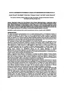
3 General Description and Characterisation of the Datasets For the purpose of this intercomparison exercise a set of modelled data had been prepared by VITO (Belgium) by applying the RIO-IFDM-OSPM model chain to the modelling domain of the city of Antwerp for the year 2012 (7). In this model chain, the RIO land-use regression model, based on the data of the official monitoring network in Belgium, provides the regional background concentration. The local increment due to traffic and industrial emissions is calculated using IFDM, a bi-Gaussian plume model designed to simulate non-reactive pollutant dispersion at a local scale. For the computation of concentrations in street canyons, the RIO-IFDM chain is furthermore coupled to the OSPM box model (8). Within the framework of the FAIRMODE intercomparison exercise, the following three monitoring sites have been selected for closer evaluation: As an example for the traffic sites: — Borgerhout II (Straatkant) (Belgium Lambert 72 coordinates: 154396 / 211055) As examples for the urban background sites: — Antwerpen-Linkeroever (Belgium Lambert 72 coordinates: 150865 / 214046) — Schoten (Belgium Lambert 72 coordinates: 158560 / 215807) A set of 341 virtual monitoring points time series with hourly data have been extracted from the RIO-IFDM-OSPM model chain outputs. The initial aim of these time series was to simulate virtual monitoring stations with daily averages for PM10, and virtual diffusive samplers with to 2-week averages for NO2 and O3. Figure 1 provides an Overview of the annual average concentration fields obtained for PM10, NO2 and O3 for the modelling year 2012. In addition, the locations or the three selected monitoring sites, and the positioning of 341 virtual monitoring points are shown. The aim of the virtual monitoring points was to extract time series with hourly data from the RIO-IFDM-OSPM model chain outputs. Table 1 summarises some general statistical characterisation of the underlying dataset. In total, time series of 341 virtual monitoring points have been extracted from the model data. These 341 virtual receptors can be distinguished into points located within streetcanyons (SC) and points located outside of street-canyons (noSC). Furthermore, the immediate modelling outputs, consisting of simulated hourly data, are aggregated into time series of 1-day averages and 14-days averages. It should be noted that the summary statistics calculated for this set of virtual monitoring points should tend to approximate, but are not necessarily exactly identical to, the means and standard deviations of the full set of gridded data.
(7) Kracht, O., Hooyberghs, H., Lefebvre, W., Janssen, S., Maiheu, B., Martin, F., Santiago, J.L., Garcia, L. and Gerboles, M. (2016): FAIRMODE Intercomparison Exercise - Dataset to Assess the Area of Representativeness of Air Quality Monitoring Stations. 267 p. JRC Technical Reports 102775. EUR 28135 EN. EUR – Scientific and Technical Research Series. ISSN 1831-9424 (online), ISBN 978-92-79-62295-3 (PDF), DOI 10.2790/479282. (8) Berkowicz, R., Hertel, O., Larsen, S.E., Sørensen, N.N., Nielsen, M. (1997): Modelling traffic pollution in streets (report in PDF format, 850 kB, http://www.dmu.dk/en/air/models/ospm/ospm_description/)
9
Figure 1. Overview of the annual average concentration fields obtained for PM10, NO2 and O3 for the modelling year 2012.
Coordinates are referring to a projection in the Belgium Lambert 72 system (EPSG: 31370). The locations of the three selected monitoring stations (Antwerpen-Linkeroever and Schoten for urban background sites, and Borgerhout-Straatkant for the traffic site) are also shown in the plots. The bottom right panel illustrates the positioning of 341 virtual monitoring points (the NO2 concentration field is repeated in the background of this panel for a better spatial orientation).
10
Table 1. Summary statistics of the time series of 341 virtual monitoring points
Simulated Hourly Data (Antwerp 2012) Virtual Number Station of Type Points
all
341
SC noSC
Grand Mean [μg/m3] PM10 NO2
Grand Standard Deviation [μg/m3]
Pooled Standard Deviations of the Individual Time Series [μg/m3]
Standard Deviation of the Annual Means of the Time Series [μg/m3]
O3
PM10
NO2
O3
PM10
NO2
O3
PM10 NO2
O3
24.7
40.0 31.2
16.0
22.3
25.3
15.8
18.2
25.0
2.3
11.8
4.1
100
26.0
49.4 30.1
16.2
21.8
24.9
16.1
18.9
24.8
1.9
10.8
2.4
241
24.1
36.1 31.7
15.8
21.2
25.4
15.6
18.0
25.0
2.3
10.0
4.5
1‐day Averages of Simulated Data (Antwerp 2012) Virtual Number Station of Type Points
all
341
SC noSC
Grand Mean [μg/m3] PM10 NO2
Grand Standard Deviation [μg/m3]
Pooled Standard Deviations of the Individual Time Series [μg/m3]
Standard Deviation of the Annual Means of the Time Series [μg/m3]
O3
PM10
NO2
O3
PM10
NO2
O3
PM10 NO2
O3
24.7
40.0 31.2
14.2
17.7
18.6
14.0
12.9
18.2
2.3
11.8
4.1
100
26.0
49.4 30.1
14.4
16.7
18.3
14.3
12.8
18.2
1.9
10.8
2.4
241
24.1
36.1 31.7
14.1
16.6
18.7
13.9
13.0
18.2
2.3
10.0
4.5
14‐days Averages of Simulated Data (Antwerp 2012) Virtual Number Station of Type Points
all
341
SC noSC
Grand Mean [μg/m3] PM10 NO2
Grand Standard Deviation [μg/m3]
Pooled Standard Deviations of the Individual Time Series [μg/m3]
Standard Deviation of the Annual Means of the Time Series [μg/m3]
O3
PM10
NO2
O3
PM10
NO2
O3
PM10 NO2
O3
24.7
40.1 31.1
9.8
13.8
13.5
9.7
7.1
13.1
2.3
11.9
4.1
100
26.0
49.5 30.0
9.8
12.7
13.1
9.8
6.9
13.1
1.9
10.8
2.4
241
24.2
36.2 31.6
9.7
12.2
13.6
9.6
7.2
13.1
2.3
10.0
4.5
Summary statistics of the time series of 341 virtual monitoring points extracted from the modelled dataset for the city of Antwerp for 2012. The total set of 341 receptor points is additionally disaggregated into points located within street-canyons (SC) and points located outside of street-canyons (noSC). The immediate modelling outputs (simulated hourly data) are compared to the aggregated time series (1-day averages and 14-days averages of simulated data).
11
The annual average concentrations of PM10, NO2 and O3 for these three groups of selected virtual monitoring points are derived by calculating the arithmetic means of the complete set of all time series of all selected receptor points (“grand mean”). The grand means of hourly data and 1-day averages are naturally exactly the same.9 In analogy to the grand mean, the overall variability of the pollutant concentrations is described by the grand standard deviation, which is likewise calculated from all time series values of all selected receptor points. This overall standard deviation includes all contributions originating from the temporal and from the spatial variability. By comparison, the “pooled standard deviation of the individual time series” reflects the inter-annual temporal variations within the individual receptor points’ time series only. To complement this, the field “standard deviation of the annual means of the time series” provides the standard deviation of the annual averages of the selected receptor points (a measure of the spatial variability within the annual average concentration field). As a general observation from these simple characterisations, the spatial variability tends to be highest for NO2, whereas the temporal variability tends to be highest for O3. For all three aggregations (hourly, daily and 14-days) the spatial variability is lowest for PM10. The temporal variability is lowest for PM10 in the case of the hourly time series. However, for the daily and for the 14-day time series the temporal variability is lowest for NO2. This change in the ranking positions with longer averaging times is probably attributable to the relatively short life-time of NO2 (stronger fluctuations observable in the hourly values which are then suppressed by the daily and 14-days averaging). In order to get a better insight into the inter-annual evolutions of the spatial concentration fields, figure 2 presents time series of the spatial mean, the spatial standard deviation, and the relative spatial standard deviation calculated for the full set of 341 virtual monitoring points. These calculations have been based on the 14-day averages time series of NO2, PM10 and O3, and on the daily averages time series for PM10. For the brevity of the illustration, a split-up into street-canyon and non-street-canyons locations has been omitted. From the time series presented in figure 2, the mean O3 concentration shows a typical continental annual cycle with a broad summer maximum. In contrast to O3, the annual variation of NO2 concentration reveals an anti-cyclic behaviour with higher levels in the winter time and a broad depression of concentrations in the summer time. The seasonal variation of PM10 is less pronounced, with elevated concentrations occurring in late winter and in spring. An important characteristic with regards to considerations on the spatial representativeness of monitoring sites is the annual evolution of the spatial variability within the concentration fields. It can be seen that the spatial variability of NO2 concentrations increases in summer time, whereas O3 shows the opposite behaviour. This is especially expressed very clearly in the relative standard deviation time series. A seasonal variation of the spatial variability of PM10 is less clearly pronounced.
9
Note that, however, the grand means of 14-day averages do not exactly match these former values, because the 26 full 14-day periods considered do not include the last 2 days of the year: the series of 14-day averages contain only 364 of the 366 days in total for the leap year 2012.
12
Figure 2. Time series of spatial mean, spatial standard deviation, and relative spatial standard deviation of virtual monitoring points.
Time series of spatial mean, spatial standard deviation, and relative spatial standard deviation of the 14day average values (left side) and 1-day average values (right side) of 341 virtual monitoring points for the modelling year 2012. These metrics reflect the overall means, the total standard deviations and total relative standard deviations of concentrations of virtual monitoring points within the full spatial extent of the model domain as can be obtained for each timestep.
13
4 Participating Teams Eleven teams from nine different countries participated in this intercomparison exercise on the spatial representativeness of air quality monitoring sites. Table 2 summarises team names, participants, and details their affiliations. Table 2. List of participating teams and institutions Team Name (Acronyms) CIEMAT
Country
ESP
Affiliations
Participants José Luis Santiago
Research Centre for Energy, Environment and Technology (CIEMAT), Madrid, Spain
Fernando Martin Antonio Piersanti
ENEA
ITA
Italian National Agency for New Technologies, Energy and Sustainable Economic Development (ENEA), Bologna, Italy
Giuseppe Cremona Gaia Righini Lina Vitali
Environmental Protection Agency (EPA), Dublin, Ireland
Kevin Delaney EPAIE
IRL
Bidroha Basu
Trinity College Dublin (TCD), Dublin, Ireland
Bidisha Ghosh FEA-AT
FI
AUT
FIN
Wolfgang Spangl
Federal Environment Agency - Austria (FEA-AT), Vienna, Austria
Christine Brendle Jenni Latikka
Finnish Meteorological Institute (FMI), Helsinki, Finland
Anu Kousa
Helsinki Region Environmental Services Authority (HSY), Helsinki, Finland
Erkki Pärjälä
City of Kuopio, Kuopio, Finland
Miika Meretoja
City of Turku, Turku, Finland
Laure Malherbe INERIS
FRA
National Institute for Industrial Environment and Risks (INERIS), Verneuil-en-Halatte, France
Laurent Letinois Maxime Beauchamp
ISSEPAWAC
Fabian Lenartz
Public Service Scientific Institute (ISSeP), Liege, Belgium
Virginie Hutsemekers
Walloon Air and Climate Agency (AwAC), Jambes, Belgium
BEL
RIVM
NLD
SLB
SWE
Lan Nguyen Ronald Hoogerbrugge Kristina Eneroth
Environment and Health Administration City of Stockholm, Stockholm, Sweden
Sanna Silvergren Peter Viaene
VITO
BEL
Netherlands National Institute for Public Health and the Environment (RIVM), Bilthoven, Netherlands
Flemish Institute for Technological Research (VITO), Mol, Belgium
Bino Maiheu Stijn Janssen
VMM
BEL
Flanders Environment Agency (VMM), Aalst, Belgium
David Roet
14
5 Spatial Representativeness Methods used by the Participants In the following, we will provide a short overview of the SR methods that have been used by the different participating teams. A more detailed compilation of full methods descriptions provided by each team can be found in ANNEX I (Documentation of Methods and Criteria). Furthermore, Table 3 (at the end of this chapter) provides a consolidated overview of the input data used by the different participating teams, whereas Table 4 and Table 5 show a breakdown of this information into input data used for traffic stations and for background station, respectively. These tables do also indicate if data additional to the shared Antwerp dataset has been used (e.g., satellite maps or street view data from different online providers). More detailed information about the particular input data files used by each team have been collected amongst the participants and are compiled in ANNEX II.
5.1 Brief methods descriptions 5.1.1 CIEMAT The methodology applied by CIEMAT (Spain) is based on annual average concentration maps obtained by means of weighted averages of Computational Fluid Dynamics simulation results (WA CFD-RANS methodology1,2) taking into account hourly averages of local meteorological observations. High-resolution average concentration maps of NO2 and PM10 are computed in a domain of 0.8 km x 0.8 km around the AQMS BorgerhoutStraatkant (traffic site). From these maps, the SR area is delimited as the area where the similarity condition for concentration is fulfilled. In this exercise, the threshold used to calculate the SR area was ± 20% of the concentration at the AQMS. References: 1 Santiago, J.L., Borge, R., Martín, F., de la Paz, D., Martilli, A., Lumbreras, J., Sanchez, B., ‘Evaluation of a CFD-based approach to estimate pollutant distribution within a real urban canopy by means of passive samplers’, Science of the Total Environment, 576, 2017, pp. 46-58, doi: 10.1016/j.scitotenv.2016.09.234. 2
Santiago, J.L., Martín, F., Martilli, A., ‘A computational fluid dynamic modelling approach to assess the representativeness of urban monitoring stations’, Science of the Total Environment 454-455, 2013, pp. 61–72, doi: 10.1016/j.scitotenv.2013.02.068.
5.1.2 ENEA Calculations by ENEA (Italy) are based on the application of the Concentration Similarity Frequency (CSF) function1, which recursively relates time series of modelled concentration fields to the concentration at the AQMS. For every time step, relative concentration differences between the AQMS and all 341 receptor points are compared with a threshold, in order to assess the condition of similarity. Finally, the SR area is delimited as the area where the similarity condition is fulfilled >90% of the time on a yearly basis. In order to obtain SR areas from the sparse CSF point values available within this IE, inverse distance weighting interpolation has been applied in an intermediate step. References: 1
Piersanti, A., Ciancarella, L., Cremona, G., Righini, G., Vitali, L., ‘Spatial representativeness of air quality monitoring stations: a grid model based approach’, Atmospheric Pollution Research, No 6, 2015, pp. 953-960, doi: 10.1016/j.apr.2015.04.005
15
5.1.3 EPAIE The method applied by EPAIE (Ireland) compared 1 year hourly concentration time series of the 341-virtual receptor points to the corresponding time series of the associated AQMS. Within the SR area the median of the 8784 concentration differences (366 days x 24 hours) should not exceed 20%. For the traffic site, the area of assessment was limited to virtual receptors within 500 m of the AQMS, while a limit of 3 km was chosen for the background AQMS. Finally, the SR area was delimitated using kriging interpolation.
5.1.4 FEA-AT Calculations of FEA-AT (Austria) are based on similarity criteria comparing the modelled annual mean concentration fields to the AQMS. The similarity thresholds (± 5 µg/m³ for NO2, ± 3 µg/m³ for PM10, and ± 4.1 µg/m³ for O3) originate from considerations about the concentration ranges observed in Europe, and have been updated for the Antwerp case. In addition, criteria for emissions are applied: For PM10 domestic heating emissions are considered (traffic emissions were found to not contribute information in addition to the concentration itself). For traffic stations, road type (motorway or not) is considered. The industrial area is separated by expert judgement based on the modelled concentration fields. References: UMWELTBUNDESAMT (2007): Spangl, W., Schneider, J., Moosmann, L. & Nagl, C.: Representativeness and classification of air quality monitoring stations – final report. Service contract to the European Commission - DG Environment Contract No. 07.0402/2005/419392/MAR/C1. Umweltbundesamt, Wien, 2007, Reports, Bd. REP-0121.
5.1.5 FI Estimations of SR areas by the FI team (Finland) are based on annual mean concentrations modelled by VITO, measurements of the AQMS’s, and data presenting their surrounding (building height & density, roughness, land-use). In addition, traffic intensity was the main input when estimating SR areas for the traffic station. For the background stations, locations of emission sources and wind direction distributions have been also considered. SR assessment is established on similarity. At the traffic station, streets with similar traffic intensity are chosen from the area with equal city structure. At the background stations, areas with similar city structure, modelled concentration and under same emission sources are chosen.
5.1.6 INERIS INERIS assessed SR areas for NO2 and PM10 on annual averages. The SR areas were estimated in two main stages. First, a spatial estimate of concentrations and concentration uncertainties (from kriging error standard deviations) was prepared. Second, NO2 and PM10 concentrations were interpolated from modelling output data applying a recently developed kriging-based approach (Beauchamp et al., 2016). This methodology is an adaptation of external drift kriging where emission data and distance to the roads are used as secondary variables to account for concentration gradients in urban areas and include traffic-related data in the map. Finally, the SR area was delimitated based on a combined criterion for maximum permissible concentration deviations (30% for NO2 and for PM10) and maximum permissible statistical risk (15% risk of wrongly including a point in the SR area).
16
References: BEAUCHAMP M., MALHERBE L., 2016. ANNEXE
TECHNIQUE AU RAPPORT INTITULÉ
ESTIMATION
DE L’EXPOSITION DES
POPULATIONS AUX DÉPASSEMENTS DE SEUILS RÉGLEMENTAIRES. INTERPOLATION DES SORTIES DE MODÈLES URBAINS PAR
KRIGEAGE AVEC DÉRIVE POLYNOMIALE.
NOTE LCSQA, HTTP://WWW.LCSQA.ORG.
Beauchamp M., Malherbe L., Létinois L., 2011. Application de méthodes géostatistiques pour la détermination de zones de représentativité en concentration et la cartographie des dépassements de seuils. Rapport LCSQA, http://www.lcsqa.org. Beauchamp M., 2012. Cartographie du NO2 à l’échelle locale, Représentativité des stations, Dépassements de seuils. Note LCSQA (complémentaire du rapport précité), http://www.lcsqa.org. Bobbia M., Cori A., de Fouquet Ch., 2008. Représentativité spatiale d’une station de mesure de la pollution atmosphérique. Pollution Atmosphérique, n°197, 63-75.
5.1.7 ISSEeP & AwAC The methods used by ISSEeP & AwAC (Belgium) are based on emission data and depend on the type of station: For traffic sites, all streets are classified into three pollution levels depending on road emissions and on how the traffic lanes are enclosed by surrounding buildings. The SR area is evaluated within a 500 m radius around the AQMS and extends to all road segments with the same emission level. For background sites, total emissions of each pollutant are first disaggregated into 100x100 m² cells, then re-aggregated through a spatially moving sum with a circular window of radius 1 km. The SR area extends to all points with total emission values similar to those at the AQMS ± a tolerance. The tolerance value in this similarity criterion is set subjectively but based on indications found in the literature1. References: 1
Spangl, W., Schneider, J., Moosmann, L. and Nagl C., Representativeness and classification of air quality monitoring stations, REP-0121, Umweltbundesamt GmbH, Austria, 2007.
5.1.8 RIVM RIVM (Netherlands) worked towards a station classification based on Principal Component analysis (PCA) together with a study of the micro/macro status of the station. In the PCA analysis the first principal component (PC1) is defined as the linear combination of the original variables that describes the maximum amount of variation present in the data set, and so on. Based on previous experience obtained with the Dutch Monitoring network1 the PCA was performed with diurnal concentration variations. The results are shown as projections of the measurement locations (score plot) and as projection of the initial variables (loadings plot) on the principle components. Similar stations appear as clusters in the score plots. References: 1
Nguyen,P.L., Stefess,G., de Jonge,D., Snijder,A., Hermans,P.M.J.A., van Loon,P., Hoogerbrugge,R., Evaluation of the representativeness of the Dutch air quality monitoring stations. The National, Amsterdam, Noord-Holland, Rijnmond-area, Limburg and Noord-Brabant networks. RIVM Report 680704021/2012,2012
5.1.9 SLB In the contribution of SLB (Sweden), SR area for the two urban background AQMS was defined as the circular buffer zone around the stations where the standard deviation of the modeled average concentration within the buffer zone was equal to a specific threshold1. The standard deviation was calculated on the set of all modeled average concentrations within the buffer zone. SR area for the traffic AQMS was defined as the part of the street where there are buildings on both sides and the traffic emissions differ
17
less than 10 % from those at the AQMS. The SR area for the traffic AQMS consists of the street canyon width plus a buffer zone of 25 m. References: 1
Lövenheim, B. Exposure to air pollution within the region of Eastern Sweden’s Air Quality Management Association. Calculations of population exposure of particulate matter (PM10) and nitrogen dioxide in 2015 (in Swedish). Eastern Sweden’s Air Quality Management Association, Report LVF 2017:12. In press, will be available at: http://slb.nu/slbanalys/rapporter/pdf8/lvf2017_012.pdf.
5.1.10
VMM
VMM (Belgium) applied a classification methodology1 which considers emissions from road traffic, domestic heating and industrial emissions, and dispersion conditions for all AQMS in the network. Population density is used as a proxy for domestic heating, and CORINE land cover data for dispersion conditions. The surrounding of the AQMS is divided into smaller sub-areas, each of which is classified (in this IE a 1100x1100 m2 grid with mesh size 100 m was chosen for subdivision). The similarity in classifications of the sub- areas and the AQMS is then quantified. Finally the SR area is calculated as the set of sub areas for which the weighted sum of a similarity indicator is above a given threshold2. References: 1
Spangl, W., Schneider, J., Moosmann, L. and Nagl, C., Representativeness and classification of air quality monitoring stations, Umweltbundesamt, Wien, 2007 2
Roet, D. and Celis, D., Life + ATMOSYS deliverable: A method for selecting monitoring stations for model validation, VMM, Belgium, 2014 http://www.atmosys.eu/faces/doc/ATMOSYS%20Deliverable%20Action%204_updateV1.1.pdf
18
Table 3. Overview of input data used by the different teams. Grey background indicates data additional to the shared Antwerp dataset. FAIRMODE CCA-1 Spatial Representativeness Intercomparison Exercise ---- Overview Table CIEMAT
ENEA
FEA-AT
FI
EPA
INERIS
ISSeP&AwAC
RIVM
SLB
VITO
VMM
Spain
Italy
Austria
Finland
Ireland
France
Belgium
Netherlands
Sweden
Belgium
Belgium
(CFD-RANS)
Totals
(PCA)
Concentrations Monitoring Stations (hourly)
X
Monitoring Stat. (only annual avg)
X
X
X
X
X
4 X
for ref (only 1st trial)
Virtual Monitoring Stations (n=341)
X
X
X
X
raw timeseries (hourly)
X
X
X
X
X
4
X
6
X
5
virtual samplers (14-day avg)
0
noisy virtual samplers (14-day avg)
1
for reference
Concentration Maps (annual avg)
X
X
X
Raw Model Outputs (annual avg)
X
X
4 1
Emissions Road Traffic
X
Domestic Heating
X
X
X
X
X (for PM10)
X
X
X
4
X
X
X
3
Industry
X
X
7
Emission Proxies Traffic Emission Proxies
road type "motorway"
X
2 from population
Domestic Heating Proxies from conc. maps
Industry Emission Proxies
1 1
Population Density
X
X
2
Dispersion Conditions Building Geometry
X
X
X
Street Width
X
4
X
Distance to Roads
X
not applied for Antwerp
Corine Landcover Classes
X
1 1 (2)
X
X
X
4
Meteorological Data Wind Velocity
X
X
2
External Information Google or Bing Satellite Images
number of lanes
X
Google Street View Data
X
Traffic Network
2 X
2
X
1
Miscellaneous used a buffer
for traffic site
a priori restricted domain
2
for traffic site
X
X
2
X
10
X
6
Final Results Polygons
X
X
X
allways contiguous also non-contiguous other types
X
X
X
X
X
X
X
X
X
gridded values
X X PCA classification
19
X
X
X
X
4 2
Table 4. Overview of input data used by the different teams for traffic sites. Grey background indicates data additional to the shared Antwerp dataset. FAIRMODE CCA-1 Spatial Representativeness Intercomparison Exercise ---- Overview Table (Traffic Sites) CIEMAT
ENEA
FEA-AT
FI
EPA
INERIS
ISSeP&AwAC
RIVM
SLB
VITO
VMM
Spain
Italy
Austria
Finland
Ireland
France
Belgium
Netherlands
Sweden
Belgium
Belgium
(CFD-RANS)
Totals
(PCA)
Concentrations Monitoring Stations (hourly)
X
Monitoring Stat. (only annual avg)
X
X
X
X
X
4 X
for ref (only 1st trial)
Virtual Monitoring Stations (n=341)
X
X
X
X
raw timeseries (hourly)
X
X
X
X
X
4
X
6
X
5
virtual samplers (14-day avg)
0
noisy virtual samplers (14-day avg)
1
for reference
Concentration Maps (annual avg)
X
X
X
Raw Model Outputs (annual avg)
X
X
4 1
Emissions Road Traffic
X
Domestic Heating
X
X
X
X (for PM10)
X
X
3
X
X
2
Industry
X
X
X
7
Emission Proxies Traffic Emission Proxies
road type "motorway"
X
2 from population
Domestic Heating Proxies from conc. maps
Industry Emission Proxies
1 1
Population Density
X
X
2
Dispersion Conditions Building Geometry
X
X
X
Street Width
X
4
X
Distance to Roads
X
not applied for Antwerp
Corine Landcover Classes
1 1 (2)
X
X
X
3
Meteorological Data Wind Velocity
X
1
External Information Google or Bing Satellite Images
number of lanes
X
Google Street View Data
X
Traffic Network
2 X
2
X
1
Miscellaneous used a buffer
X
a priori restricted domain
X
2
X
X
2
X
10
X
6
Final Results Polygons
X
X
X
allways contiguous also non-contiguous other types
X
X
X
X
X
X
X
X
X
gridded values
X X PCA classification
20
X
X
X
X
4 2
Table 5. Overview of input data used by the different teams for background sites. Grey background indicates data additional to the shared Antwerp dataset. FAIRMODE CCA-1 Spatial Representativeness Intercomparison Exercise ---- Overview Table (Background Sites) CIEMAT
ENEA
FEA-AT
FI
EPA
INERIS
ISSeP&AwAC
RIVM
SLB
VITO
VMM
Spain
Italy
Austria
Finland
Ireland
France
Belgium
Netherlands
Sweden
Belgium
Belgium
(CFD-RANS)
Totals
(PCA)
Concentrations Monitoring Stations (hourly)
X
X
Monitoring Stat. (only annual avg)
X
X
X
3 X
for ref (only 1st trial)
Virtual Monitoring Stations (n=341)
X
X
X
X
raw timeseries (hourly)
X
X
X
X
X
4
X
6
X
5
virtual samplers (14-day avg)
0
noisy virtual samplers (14-day avg)
1
for reference
Concentration Maps (annual avg)
X
X
X
Raw Model Outputs (annual avg)
X
X
4 1
Emissions Road Traffic X (for PM10)
Domestic Heating Industry
X
X
X
X
X
X
X
4
4
X
X
X
3
Emission Proxies Traffic Emission Proxies
1
road type "motorway"
from population
Domestic Heating Proxies from conc. maps
Industry Emission Proxies
1 1
Population Density
X
X
2
Dispersion Conditions Building Geometry
X
1
Street Width
0
Distance to Roads
X
not applied for Antwerp
Corine Landcover Classes
X
1 (2)
X
X
X
4
Meteorological Data Wind Velocity
X
1
External Information Google or Bing Satellite Images
X
Google Street View Data
1
X
Traffic Network
X
2
X
1
Miscellaneous used a buffer
0
a priori restricted domain
X
X
2
Final Results Polygons
X
X
allways contiguous also non-contiguous
X
X
X
X
X
X
X
X
X X
21
X X
X
9 4
X PCA classification
other types
X X
5 1
6 Reporting of Data and Results Within the IE, the 11 participating teams delivered SR estimates for the pollutants PM10 and NO2 at one traffic site (Borgerhout-Straatkant, corresponding to virtual station location v216), and for PM10, NO2 and O3 at two urban background sites (Antwerpen-Linkeroever and Schoten, corresponding to virtual station location v7 and v17, respectively). Table 6 provides a detailed overview of the sets of results received from the different teams. From this table it can be seen that 10 teams delivered polygons f SR areas surrounding the stations under investigation, whereas one team (RIVM) rather worked towards a classification of the stations by principal component analyses (PCA). On top of these mandatory tasks, some teams provided additional results that had been suggested as optional tasks following discussions at the previous FAIRMODE technical meeting in Zagreb (27-29 June 2016). In specific, four teams provided additional SR estimates for the 8 virtual stations v43, v63, v68, v88, v105, v115, v135 and v137. Furthermore, two teams provided also a classification of the 3 + 8 virtual stations. However, as the response to these optional tasks was only from a smaller part of the participants group, the evaluation of these additional data will not be part of this present report. These additional data can nevertheless be useful for further investigations in the future.
22
Table 6. Overview of results received from the different teams FAIRMODE CCA-1 Spatial Representativeness Intercomparison Exercise ---- Overview Table CIEMAT
ENEA
FEA-AT
FI
EPA
INERIS
ISSeP&AwAC
RIVM
SLB
VITO
VMM
Spain
Italy
Austria
Finland
Ireland
France
Belgium
Netherlands
Sweden
Belgium
Belgium
X
X
X
X
X
X
X
X
X
X
10
X
X
X
X X
6
Totals
Final Results Polygons allways contiguous also non-contiguous other types
X
X
X
X
X
4
PCA classification
gridded values
2
3 Primary Stations VS 216 (Borgerhout - traffic) NO 2
X
X
X
X
X
X
X
X
X
X
X
11
PM10
X
X
X
X
X
X
X
X
X
X
X
11
O3
no
no
no
no
no
no
no
no
no
no
no
0
VS 7 (Linkeroever - background) NO 2
no
X
no
X
X
X
X
no
X
X
X
8
PM10
no
X
X
X
X
X
X
X
X
X
X
10
O3
no
X
no
no
no
no
X
no
X
X
no
4
VS 17 (Schoten - background) NO 2
no
X
X
X
X
X
X
X
X
X
X
10
PM10
no
X
X
X
X
X
X
X
X
X
X
10
O3
no
X
X
X
X
no
X
X
X
X
no
8
8 Additional Stations SR area
no
X
X
no
no
X
no
no
no
X
no
4
classifications
no
no
X
no
no
no
no
X
no
no
no
2
23
7 Quantitative Outcomes of the Intercomparison 7.1 Methods and procedures followed by the participants The SR methodologies applied within this exercise can roughly be distinguished as methods relying on air quality measurements, methods relying on proxy data, and methods relying on air quality model outputs. However, certain overlap between these categories exists. From a rough categorisation based on the selection of input data, 4 out of the 11 teams deployed the high resolution annual average concentration fields, which was made available from the RIO-IFDM-OSPM model chain outputs on a 5x5 m2 regular grid, as an immediate starting point (FEA-AT, FI, SLB and VMM). In contrary, 2 teams (ENEA and EPA-IE) performed an interpolation similarity criteria applied to time series of the 341 modelled virtual stations, and one team (INERIS) performed a geostatistical interpolation of the annual average raw model outputs (which were available on an irregular grid). Furthermore, 2 teams primarily focused on the use of concentration proxies (ISSEPAWAC and VMM), one team deployed their own computational fluid dynamics (CFD) model (CIEMAT), and one team worked on principal component analyses (PCA) of concentration measurements (RIVM).
7.2 SR area estimates Some selected examples of different SR estimates obtained within this intercomparison exercise are exemplified in Figure 3 (NO2 at site v7), Figure 4 (O3 at site v7) and Figure 5 (PM10 at site v7). For the brevity of this chapter and in aiming to save space, only a small excerpt of the comprehensive results can be shown here. A complete compilation of maps for all SR area estimates can be found in Annex III (spatial representativeness maps organised by team) and in Annex IV (spatial representativeness maps organised by pollutant & station). Figure 3. Examples of SR area estimates obtained for NO2 at the urban-background site Antwerpen-Linkeroever (site v7).
Left: estimate obtained by the team FI (2.47 km2), Right: estimate obtained by INERIS (131 km2); green background colours depict the annual average concentration field of NO2. The position of the AQMS AntwerpenLinkeroever is highlighted in red. The actual SR areas are described by the grey coloured fields in the foreground.
24
Figure 4. Examples of SR area estimates obtained for O3 at the urban-background site Schoten (site v17).
Left: estimate obtained by EPAIE (37.1 km2), Right: estimate obtained by FEA-AT (333 km2); green background colours depict the annual average concentration field of O3. The position of the AQMS Schoten is highlighted in red. The actual SR areas are described by the grey coloured fields in the foreground.
Figure 5. Examples of SR area estimates obtained for PM10 at the traffic site BorgerhoutStraatkant (site v216).
Left: estimate obtained by VITO (395 km2), Right: estimate obtained by VMM (0.47 km2); orange background colours depict the annual average concentration field of PM10. The position of the AQMS Borgerhout-Straatkant is highlighted in red. The actual SR areas are described by the grey coloured fields in the foreground.
25
7.3 Size of the SR areas For ENEA, EPAIE, FEA-AT, FI, INERIS, ISSEPAWAC, SLB, VITO and VMM surface areas could be immediately calculated from the shapefiles (containing single and/or multipart polygons) delivered by these teams. Yet, two exceptions for SR area size calculations exist for the teams CIEMAT and RIVM: In the case of CIEMAT the original mesh of the computational fluid dynamics (CFD) simulations is an irregular grid, having a resolution of 1m x 1m close to the investigated station. The CFD model is 3-dimensional and data have been extracted at the height of the plane z = 3m (which was assumed to be more or less the height of the measurements of the air quality monitoring station). From this CFD grid extractions, SR areas for the site v216 can be directly directly computed to be 0.03178 km2 (NO2) and 0.04595 km2 (PM10). In a later step, for the purpose of reporting the results to the intercomparison exercise in the format of raster- and shape-files, results from the original CFD mesh were converted onto a regular grid with a horizontal resolution of 2m x 2m. SR areas calculated from this secondary raster files finally yield slightly smaller values, which amount to 0.02595 km2 (NO2) and 0.03716 km2 (PM10). These secondary results are however assumed to be less accurate than those areas obtained from the primary CFD grid. Results in the table therefore are those values from the primary CFD grid. The RIVM team worked towards a station classification based on PCA, which naturally does not immediately provide an SR area. RIVM pointed out that in the Dutch system concentration levels are mainly determined by modelling and direct application of a measured value is usually only recommended in the small area that is comparable with the modelling resolution. In order to (i) obtain provisional SR area sizes that could be compared within this exercise, and to (ii) estimate the number of inhabitants within the SR areas later on, it was assumed that the geometry of the traffic station is such that it is representative of (at least) 100 meters of street (as required by ANNEX III of the European Directive 2008/50/EC). The area of representativeness was then assumed to be (at least) 100*5*2 m2 (5 meters at both sides of the street), equalling 0.001 km2. For the background stations, a representative area of (at least) 1 km2 was assumed (the AQD formulates “several square kilometres” in ANNEX III with regards to NO2 and PM10, and “a few km2” in ANNEX VIII for O3). Finally, Table 7 provides a complete overview of all spatial representativeness estimates (SR area in km2) which have been obtained by the different teams for the pollutants NO2, O3 and PM10 at the urban-background sites Antwerpen-Linkeroever (v7) and Schoten (v17), and at the traffic site Borgerhout-Straatkant (v216). The quantitative SR area data are also displayed in a summary strip chart (Figure 6). From this chart, it can immediately be seen that the results obtained by the different teams revealed a considerable range of variation of the SR estimates. More detailed graphical information can be obtained from a series of bar charts (Figure 7, Figure 8 and Figure 9), which compare the total surface areas of the SR estimates by pollutant and site. These bar charts are sorted in descending order by the size of the SR area. Names of the reporting teams can be distinguished from the x-axis. In cases where no results have been reported for that combination of site and pollutant, the team names are parenthesised and follow in alphabetical order.
26
Table 7. Overview of spatial representativeness estimates (SR area in km2) obtained for the pollutants NO2, O3 and PM10 at the urban-background sites Antwerpen-Linkeroever (v7) and Schoten (v17), and at the traffic site Borgerhout-Straatkant (v216).
Pollutant: Receptor point:
NO2 v7
v17
v216
v7
v17
PM10 v216
v7
v17
v216
estimated SR areas [km2]
Participants CIEMAT
O3
NA
NA
0.03
NA
NA
NA
NA
NA
0.05
ENEA
2.65
1.70
0.10
71.36
133.0
NA
464.9
534.3
157.1
EPAIE
NA
27.44
3.44
NA
37.06
NA
37.68
37.68
3.39
FEA-AT
NA
159.9
2.06
NA
332.8
NA
257.5
118.5
0.52
2.47
58.60
0.57
NA
117.2
NA
32.01
58.60
16.69
130.8
69.90
4.37
NA
NA
NA
628.4
700.0
417.5
7.95
71.54
0.19
7.95
71.54
NA
12.84
99.61
0.19
NA
>1
> 0.001
NA
>1
NA
>1
>1
> 0.001
SLB
27.13
19.89
0.06
138.1
18.75
NA
26.71
14.12
0.06
VITO
176.0
269.4
160.0
160.0
397.0
NA
442.8
465.2
395.2
VMM
1.21
1.21
0.63
NA
NA
NA
1.21
1.21
0.47
FI INERIS ISSEPAWAC RIVM
Figure 6. Summary chart of spatial representativeness areas (SR area in km2) obtained for the pollutants NO2, O3 and PM10 at the urban-background sites Antwerpen-Linkeroever (v7) and Schoten (v17), and at the traffic site Borgerhout-Straatkant (v216).
27
Figure 7. Spatial representativeness area estimates (SR area in km2) obtained for the pollutant NO2 at the urban-background sites Antwerpen-Linkeroever (v7) and Schoten (v17), and at the traffic site Borgerhout-Straatkant (v216). The bars are sorted in decreasing size of SR-areas. Parenthesised team names indicate that no results have been reported for that combination of site and pollutant.
28
Figure 8. Spatial representativeness area estimates (SR area in km2) obtained for the pollutant O3 at the urban-background sites Antwerpen-Linkeroever (v7) and Schoten (v17). The bars are sorted in decreasing size of SR-areas. Parenthesised team names indicate that no results have been reported for that combination of site and pollutant. SR areas for O3 have not been estimated at the traffic site Borgerhout-Straatkant (v216).
29
Figure 9. Spatial representativeness area estimates (SR area in km2) obtained for the pollutant PM10 at the urban-background sites Antwerpen-Linkeroever (v7) and Schoten (v17), and at the traffic site Borgerhout-Straatkant (v216). The bars are sorted in decreasing size of SR-areas. Parenthesised team names indicate that no results have been reported for that combination of site and pollutant.
30
7.4 Population within the SR areas Participants were furthermore asked to provide estimates for the number of inhabitants within their calculated areas of representativeness. In this second step, most of the teams decided to compute zonal statistics for the population within the SR areas by overlaying the SR-area polygons with a population density raster file which was provide on a 100 m x 100 m grid. However, two teams (CIEMAT and RIVM) followed slightly different approaches adapted to the specific structure of their SR outcomes: As a consequence of the CFD approach used by the CIEMAT team, areas covered by buildings have by principle not been part of their estimated SR area. For calculating the amount of population within the SR area, the gridded population density data therefore needed to be adjusted beforehand to correct for the proportion of built-up areas within in each grid cell. In this way, the CIEMAT team re-allocated the part of the population density that was intersecting with the built-up area to the open area of each grid cell. Afterwards these adjusted population density data could be intersected with the SR-area polygons as described before. The RIVM team worked towards a station classification based on PCA. As already explained in section 7.3, it was then assumed that the geometry of the traffic station is such that it is representative of (at least) 100 meters of street, as required by the AQD. For background stations a representative area of 1000x1000 meters was assumed, and then intersected with the population density information. The numbers of inhabitants within the SR areas stated by RIVM are therefore providing a lower limit (>=), as opposed to the finite numbers derived by the other teams. Bar charts presented in Figure 10, Figure 11 and Figure 12 recapitulate the numbers of inhabitants within the areas of representativeness. Names of the reporting teams can be distinguished from the x-axis. The bar charts are sorted in descending by the magnitude of the population within the SR areas. In cases where no results have been reported for that combination of site and pollutant, the team names are parenthesised and follow in alphabetical order. It has to be pointed out that the estimates concerning the size of the SR area and the results obtained for the number of inhabitants within these SR areas cannot be linked immediately to each other in a simple linear way. The relationship between these two different strata of the final results is in fact rather complex, as it emanates from the intersection of (i) SR areas that do not only differ in the extent of their perimeter, but also in their exact shape and position, with (ii) a spatially distributed and heterogeneous population density field.
31
Figure 10. Number of inhabitants within the estimated areas of representativeness (population in thousands) obtained for the pollutant NO2 at the urban-background sites Antwerpen-Linkeroever (v7) and Schoten (v17), and at the traffic site Borgerhout-Straatkant (v216). The bars are sorted in decreasing size of population in within the SR-areas. Parenthesised team names indicate that no results have been reported for that combination of site and pollutant.
32
Figure 11. Number of inhabitants within the estimated areas of representativeness (population in thousands) obtained for the pollutant O3 at the urban-background sites Antwerpen-Linkeroever (v7) and Schoten (v17). The bars are sorted in decreasing size of population in within the SR-areas. Parenthesised team names indicate that no results have been reported for that combination of site and pollutant. SR areas for O3 have not been estimated at the traffic site Borgerhout-Straatkant (v216).
33
Figure 12. Number of inhabitants within the estimated areas of representativeness (population in thousands) obtained for the pollutant PM10 at the urban-background sites Antwerpen-Linkeroever (v7) and Schoten (v17), and at the traffic site Borgerhout-Straatkant (v216). The bars are sorted in decreasing size of population in within the SR-areas. Parenthesised team names indicate that no results have been reported for that combination of site and pollutant.
34
7.5 Further instruments of the intercomparison 7.5.1 Incremental intersections Total unions and stepwise sequential intersections of the SR area estimates (incremental intersections) have been computed and evaluated by pursuing the following principals: For each particular site and pollutant: 1) Form the union of all SR area estimates obtained by all participants. 2) Take the largest individual SR estimate and intersect it with the union. 3) Take this intersection as the new (reduced) union. 4) Take the second largest individual SR estimate and intersect it with the reduced union. 5) Take this intersection as the new (shrunken) union. 6) … continue likewise 7) Finally reaching the intersection of all estimates. The complete set of incremental intersections maps can be found in Annex V (incremental intersection maps by pollutant & station). A summary of this analysis is given in Table 8, where the total union is compared to the final intersection of all estimated SR areas for each combination of site and pollutant. For the theoretically ideal case of full agreement in-between a set of SR area estimates, total union and complete intersection should be identical. For the results of this intercomparison exercise, total union and complete intersection are yet typically separated by several orders of magnitude. Table 8. Results of the intersection analysis: areas of the total union and the final intersection of all SR area estimates.
NO2
O3
PM10
[km2]
v7
v17
v216
v7
v17
v216
v7
v17
v216
all
240
354
161
233
482
-
636
718
458
all
0.05
0.19
0.00
0.77
2.54
-
0.16
0.49
0.01
All areas are in km2.
35
7.5.2 Mutual comparisons of the level of agreement Mutual comparisons of the SR area estimates by calculations of the mutual level of agreement indicator (MLA) function have been established based on the following definition:
| |
1| ∩ | 1| ∪ |
1| 1|
As by its general principal, the MLA indicator converges to 1 for full agreement between area 1 and area 2. In contrary, it converges to 0 for no agreement between area 1 and area 2. Figure 13 demonstrates an example for the pairwise MLA indicator function calculated for the SR area estimates of ENEA and EPAIE for O3 at position v17. The SR area estimated by ENEA is shown in brown colour, whereas the SR area estimated by EPAI is shown in grey. The intersection of both estimates is depicted in red. In this example, the MLA amounts ca 10%, Figure 13. Example of the MLA indicator calculated between ENEA and EPAIE for O3 at the urbanbackground site Schoten (site v17).
The complete set of mutual comparison maps and MLA indicator calculations can be found in Annex VI (mutual comparison maps by pollutant & station). Detailed numerical summaries of the MLA evaluation can be obtained from a series of bar charts (Figure 14, Figure 15, Figure 16 and Figure 17), which summarise the calculated MLA values by pollutant and site. The bar charts are sorted in descending order by the level of agreement within between the paired SR area estimates. Names of
36
the paired teams are shown on the x-axis. In cases where no results have been reported for that combination of site and pollutant by at least one of the teams in a pair, the MLA could not be calculated. These paired team names are parenthesised and follow in alphabetical order. The results from the mutual comparisons of the level of agreement can be summarised as follows:
Values for all MLA indicators are rather low in general.
Median MLAs are always clearly < 10% for the whole set of comparisons.
A deduced ranking in terms of the order of paired similarities should be taken with care and is probably not reasonably conclusive.
37
Figure 14. MLA indicators (pairwise level of agreement) of the SR estimates obtained for NO2 at the urban-background sites Antwerpen-Linkeroever (v7) and Schoten (v17), and at the traffic site Borgerhout-Straatkant (v216). The bars are sorted in decreasing size of MLA levels. Parenthesised paired team names indicate that no SR results have been reported for this combination by at least one of the teams in a pair.
38
Figure 15. MLA indicators (pairwise level of agreement) of the SR estimates obtained for O3 at the urban-background sites Antwerpen-Linkeroever (v7) and Schoten (v17). The bars are sorted in decreasing size of MLA levels. Parenthesised paired team names indicate that no SR results have been reported for this combination by at least one of the teams in a pair.
39
Figure 16. MLA indicators (pairwise level of agreement) of the SR estimates obtained for PM10 at the urban-background sites Antwerpen-Linkeroever (v7) and Schoten (v17), and at the traffic site Borgerhout-Straatkant (v216). The bars are sorted in decreasing size of MLA levels. Parenthesised paired team names indicate that no SR results have been reported for this combination by at least one of the teams in a pair.
40
41
Figure 17. Lumped MLA indicators obtained by combining MLAs for all three pollutants (NO2, O3 and PM10) at all three sites v7, v17 and v216 (top panel ), and at the two background sites v7 and v17 (bottom panel), respectively. The bars are sorted in decreasing size of MLA levels..
42
8 First Evaluation and Interim Analysis of the Results The outcomes of the IE are providing quantitative evidence for a large variation in between the results obtained by the range of different contemporary methods. The considerable spread of the results obtained by the different teams nevertheless concerns the extent and position of the estimated SR area perimeters, but also the technical procedures and the extent of input data effectively used. In fact, though the general concept of the area of SR proved to be a useful indicator to work with, some important differences revealed regarding the details of the underlying concepts and definitions employed. These differences require detailed evaluations in order to identify the major factors triggering and controlling this variability, which could be found amongst: ‒
the basic principles of the methods
‒
the effective use of different types of input data (different choices made for subsets used from the entire data available)
‒
the parameterisation of the similarity criteria and thresholds
‒
the underlying conceptualisations and detailed definitions of SR
We consider that the diversity observed in this exercise requires the experts community to take further efforts towards a ‒
more harmonised definition representativeness”, and
of
the
concept
of
“the
‒
consistent and transparent criteria used for its quantification,
area
of
in this way eliminating unnecessary differences in the SR methodologies. Furthermore, from a methodological point of view, it was an important observation that even on a shared dataset, individual teams made a clearly diverse choice on those subsets of the data (average concentrations, concentration time series, emissions, population densities, traffic, land cover, building geometries, etc.) that had been substantial or supportive to their particular SR method. It should deserve a closer look, as how far this indicates that harmonised recommendations should be established for the input requirements of SR assessments, too.
43
9 Follow-Up Activities (Concluded) With a view of harmonisation in the field of SR, the IE also provided an excellent opportunity for the exchange of knowledge on this subject, which was organised in the form of a 1½-day workshop in conjunction with the FAIRMODE technical meeting in Athens (June 2017). The revelation of the diversity in the SR results opened a very insightful and constructive discussion. In fact, from having worked on the same shared dataset, participants of the IE were able to efficiently exchange background information in a much more detailed way as compared to what would have been feasible without this common ground. Participants of the IE agreed that the diversity of the results requires us to take further efforts towards the quantitative definition of the concept of “the area of representativeness” and in eliminating unnecessary differences in the SR methodologies. Questions that have been elaborated in more detail during the follow-up of the IE therefore included: 1. What are the future needs for harmonisation and for establishing a common frame of reference? 2. Is there a future need for standardisation, too? 3. Beyond standardisation, should the regulators / political bodies make the use of standards mandatory? 4. Would it conversely be preferable to have at disposal a set of transparent definitions and practical guidelines, but maintaining the freedom of choosing the most appropriate procedures for the different particular purposes and applications? A general consensus was found amongst participants of the IE: ‒
Currently it would not (yet) be reasonable to start discussing about (2) or (3).
‒
For the mid term objectives, the efforts of the experts community should rather be directed towards (4) first.
In the view of the organisers of this IE, it has to be pointed out that this objective will first require establishing a common framework for SR definitions and SR similarity criteria, and for harmonising the related terminologies. Even if different purposes of estimating SR might cause some conflict of goals, there is a substantial room for improvements towards a higher transparency and the need for a better comparability of SR estimates. Further to the workshop in Athens, participants were asked to prepare a brief sum-up file on their individual summaries & conclusions from the workshop and from the SR intercomparison exercise. The complete set of these contributed Individual Summaries & Conclusions can be found in Annex VII. These summary files provide a valuable overview of opinions about the current state of the art and about future directions within this FAIRMODE group. Following his particular role as being the main organiser of the SR intercomparison exercise and of the SR workshop, Oliver Kracht also worked out an extended conclusions file, which provides a comprehensive overview on the current state of these activities, and the general summary and conclusions, presented in the following chapter (chapter 10).
44
10 Conclusions About the IE and Current State of Work on SR Within the Expert Community This chapter has been worked out as the summary and conclusion of Oliver Kracht, as being the main organiser of intercomparison exercise and of the FAIRMODE activities on SR. The following sections thus give the JRC’s views on the outcome of the IE.
10.1 Introduction and general remarks The assessIment of the spatial representativeness of air quality monitoring stations is an important subject that is linked to several highly topical areas, including risk assessment and population exposure, the design of monitoring networks, model development, model evaluation and data assimilation. Nevertheless, European regulations lack a clear provision to evaluate the spatial representativeness of the stations. Also in the scientific literature, there is no unified agreement to address this complex problem. Indeed, spatial representativeness (SR) of air quality monitoring stations has been investigated and discussed intensively in the past within FAIRMODE and AQUILA. However, no well-established procedure for assessing SR has been identified so far. Also in the scientific literature, there is no unified agreement to address this complex problem. With a view of harmonisation in this field, the recently concluded intercomparison exercise (IE) on the SR of air quality monitoring sites thus also provided an excellent opportunity for the exchange of knowledge on this subject, which was organised in the form of a 1½-day workshop. The main objective of the IE was to evaluate the possible variety of SR results obtained by applying the range of different contemporary approaches to a jointly used example case study. As the working basis, a shared dataset has been selected among a set of modelling data from the city of Antwerp. All participating teams worked by using their own selected methods and by using those parts of the dataset that they would normally require. Therefore, the aim of the IE was less to see how the different methods perform. This would in fact not have been possible, as by principle a known SR reference value (“true value”) was missing. We thus rather intended to investigate how the outcomes of different approaches would compare to each other, in this way measuring consistency rather than correctness. Thereby two fundamental questions needed to be addressed: Are the different SR methods actually targeting the same metric? Or, conversely, do the professionals probably speak about several different concepts and quantities when they name it SR? In fact, the results of the IE revealed a considerable range of variation between the SR estimates - not only in terms of the size and position of the SR perimeters, but also in the technical procedures and the extent of input data effectively used. For the workshop, the revelation of this diversity opened a very insightful and constructive discussion. In fact, from having worked on the same shared dataset, participants were able to efficiently exchange background information in a much more detailed way as compared to what would have been feasible without this common ground. This was supported by well-prepared individual presentations of all participating teams. In the course of the workshop, the major factors triggering and controlling the observed spread of the SR results have been identified amongst: 1. the basic principles of the methods 2. the effective use of different types of input data (different choices made for subsets used from the entire data available) 3. the parameterisation of the similarity criteria and thresholds 4. the underlying conceptualisations and definitions of SR The conclusions that can be drawn from the IE and from the discussions at the workshop underline the need for (i) a more harmonised definition of the concept of “the area of
45
representativeness” and (ii) for consistent and transparent criteria used for its quantification. In the following sections, we will provide our detailed summary and conclusions on the particular task and key points that have been addressed during the workshop. We will also outline the opportunities for making progress towards a more harmonised quantification of SR.
10.2 Integration time scales Unsurprisingly, large agreement exists across the expert community that when assessing the SR of an AQMS, specific areas of SR need to be defined for the different pollutants. Also with regard to the different integration time scales (e.g., annual averages as opposed to daily mean values) it is commonly accepted that these do imply a different extent of the related SR areas, and that consequently customised definitions should be needed for the test statistics and for the similarity criteria. However, contrasting to the specific adoptions considered for the pollutants, it is not always clear if and how the existing SR approaches do actually include provisions for the aforementioned differences in the time scales. In particular with regards to the use of information related to the dispersion conditions (e.g., the street canyon topography and the built-up situation, but also land use in general), it gets not immediately clear how these can be quantitatively linked to a specific integration time scale (though this link might seem obvious from a qualitative point of view). To our opinion, integrating these data and establishing this relationship would ultimately best be done by the use of a suitable air quality simulation model. Similar considerations regarding the integration time scales naturally apply to the use of emission proxies, but to a certain extent also to the use of emission data in general. From a conceptual point of view, it is clear that integrating these types of information should improve the delimitation of the SR areas. However, it is difficult to quantify the level of improvement, and to conclude about the effective time scale to which this finally applies. Explicit versus effective (implicit) integration time scales: In conclusion, it seems sometimes challenging to conclude on the effective integration time scale of a methodology, which might differ from the integration time scale explicitly declared. Furthermore, comparing the approaches of different teams, in some cases it is not finally clear as how far the effects of different integration time scales get compensated (at least in part) by the selection of more strict or less strict similarity criteria. Example given, ENEA evaluated concentration differences between the AQMS and the virtual monitoring points on a time bases specifically adapted to the regulatory requirements for each particular pollutant (hourly for NO2, daily maximum of 8 hours running average for O3, daily average for PM10). EPA-IE, on the other hand, chose a unique time bases (hourly) for all three pollutants. For verifying similarity, both teams used a 20% threshold criterion with regard to the concentration differences of the single time steps. However, whereas ENEA deployed a second (frequency-based) criterion targeting the 90% percentiles of the one-year time series, EPA-IE chose this second criterion to assess the medians (i.e. the 50% percentiles). Following these considerations, it is obvious that for NO2 both teams worked on the same integration time basis (hourly), but with very different frequency criteria (90% percentiles as opposed to the less strict 50% percentiles). For O3 and for PM10 the comparison is yet more complex: The larger integration times chosen by ENEA lead to an effectively less strict thresholding operation as compared to the hourly bases chosen by EPA-IE. However, the 90% percentiles frequency criterion chosen by ENEA is more stringent than the 50% percentiles deployed by EPA-IE. It remains an open question as how far these two counter-directed choices do compensate each other and how (if at all) this could be quantified. In conclusion, integration time scales, similarity criteria, and possible other criteria always need to be considered together when evaluating the outcome of the SR area determination by any method in a comparative way.
46
10.3 Integrating different types of input data and auxiliary information: With regard to the integration of input data, the methodologies applied by the different teams can roughly be distinguished into 1) methods that apply the relevant similarity criteria to concentration maps derived from an air quality model (which can be both from an existing model, or from a dedicated model simulation established for this specific purpose) 2) methods applying similarity criteria to concentration maps derived from the interpolation of measurements 3) methods relying on a simplified integration of proxy data and auxiliary information The integration of complex information from multiple sources, possibly even at different space and time scales and at varying quality levels is a challenging task. However, as already discussed in the previous section (section 10.2: Integration time scales) integration of multiple data can nowadays best be done by the use of a suitable air quality simulation model. Model outputs could further be improved by using data assimilation techniques to derive a combination of modelling and measurement data. Pros and Cons of using of air quality models to estimate SR: Different arguments concerning this aspect have been exchanged in the FAIRMODE group: Pros for deploying a (high-resolution) model: ●
A high-resolution urban air quality model seems the most adequate way to integrate all relevant influencing variables.
●
If accurate enough, such model takes into account the high spatial variability of concentrations in an urban area.
Cons of using model data: ●
Potential uncertainty and inadequate quality of the model outputs
●
Suitable type of modelling data is not available everywhere.
●
Various user groups can thus be in need of more simple estimation methods.
●
Accurate calibration and validation of (high-resolution) models might require a precise SR area estimate. This could be a vicious cycle, viewing that the SR area estimate itself requires a calibrate model beforehand.
However, we are nowadays observing a rapid increase of the availability of highresolution air quality models for many places in Europe. Growingly more modelling teams have the expertise and technical capacities to apply this kind of simulation techniques. Against this background, it can be expected that the aforementioned need for rather simplified alternatives will steadily decrease. On the other hand, notwithstanding the actual availability of the modelling tools, the availability of suitable input data (e.g., traffic volumes at line segments) might still be a different limiting factor.
10.4 Similarity criteria In this exercise, both absolute and relative similarity criteria have been applied. Absolute similarity criteria can more easily be linked to certain regulatory requirements. Example given, ANNEX I of the 2008/50/EC directive might serve as a model. Table A of this ANNEX I in fact provides data quality objectives for ambient air quality assessment. These data quality objectives are expressed as percentages, but according to the directive they shall be interpreted as being applicable in the region of the appropriate 47
limit value. Such percentage of an absolute value (the limit values), would thus result into an absolute criterion. Relative similarity criteria are, on the other hand, more suitable for assessing the full concentration range within a fluctuating time series. However, relative similarity criteria can be problematic in the low concentration ranges. Following these considerations, we propose that a combined absolute / relative similarity criterion would be the better choice. Example given, a mathematical rule for such similarity criterion δ could be defined as the max of [± xx µg/m3] and [± yy% of the observed concentration].
10.5 What are the controlling factors for the SR estimates From our intercomparison exercise we obtained very interesting insights about how SR estimates obtained by different experts can differ. Wide difference could be observed not only in size and extent, but also in the location and shape of the SR areas. Thereby the teams have worked on a common shared dataset, but using their own individual methods and their own particular similarity criteria and threshold values. The IE thus concerned the full user manipulable parameter space, including (i) the choice of a subset from the data available, (ii) the SR method as such, (iii) the similarity criteria definitions, and (iv) the parameter values chosen for these similarity criteria. However, current outputs do not enable us to distinguish between the individual influences of these different groups of parameters: In fact we did not explicitly investigate and consequently have less clear information about how SR results would vary when manipulating only one of the aforementioned factors (i) to (iv) while keeping the others fixed. Example given, from our available results it is thus difficult to conclude about the sensitivity of a particular method to the different possible choices for the similarity criteria parameters. It becomes evident that certain further evaluations would be helpful to provide more quantitative evidences for the discussions and to support the process harmonisation. In order to better support the future discussion on prospectively harmonised similarity criteria and methodological recommendation, we suggest that further quantitative investigations would be of immediate interest: ●
How does the parameterisation of the similarity criteria/threshold values quantitatively influence the estimation of SR areas?
●
How does the choice of additional criteria (i.e. should SR area be contiguous or not) quantitatively influence the estimation of SR areas?
Such investigations could be based on simple variations of parameter values and / or more systematically by Monte Carlo simulations. The outcomes of this assessment could then be turned into a sensitivity analysis and aid to distinguish regions within the parameter space which are more influential on the SR results from those where a variation of the similarity criteria does only cause lesser or negligible effects. Practically this type of analysis would best be done based on a fully automated formalisation of one or more selected methods into a suitable computer code. It should be pointed out that the analyses proposed here would be important to be conducted before getting into serious discussion about the selection of parameter values for the similarity criteria. In this way we would a-priori be able to avoid being trapped into conceptual discussions on the selection of similarity criteria, without knowing if there were important practical constraints potentially overruling the theoretical considerations. Beyond these immediate needs, such integrated code would also be useful for further works in the mid-term future, example given to investigate questions like:
48
●
Can we demonstrate how SR evolves over the evaluation period (examples given time series of daily SR areas over a year, time series of SR for the hours of the day – i.e. 24 averages of 365 hours)?
●
Can the SR codes be inverted to identify optimal station positions?
10.6 Population within the SR area To estimate the amount of population for which a monitoring station is representative one needs to intersect SR areas with the population density. In this exercise, population density in turn constituted a spatially distributed and heterogeneous raster field. Estimates for the size of the SR area and the number of inhabitants within the SR areas can therefore not be linked in a simple linear way. Participants of the IE have thus been asked also to report the number of inhabitants coupled to their estimates of SR areas. This was relevant for inspecting as to what extent prospective incongruence in the SR areas would translate to a comparable incongruence in the population estimates. Example given, if the spatially incongruent portions of the SR area estimates (i.e. those parts of the SR areas that do not intersect within between participants) would have mainly concerned very low populated or even non-populated areas, this disagreement in SR areas would probably have been less relevant. During the workshop, participants suggested to take a closer look at this matter. We therefore further followed up on this analysis after the workshop. The analysis however confirmed that also with a view on population the overall picture of the intercomparison results is not fundamentally different from the conclusions already obtained for the areas. In fact, the estimates for the size of population within the SR areas do reveal a similar level of diversity as the SR area estimates themselves. As a general remark, it should be noted that the evaluation of population data by intersecting SR areas and population density is of course already a certain simplification in itself. It assumes a static relationship, whereas in reality people in a city do actually move around in more or less complicated ways, thereby entering or leaving the SR area of a monitoring station in a complex temporal pattern.
10.7 Miscellaneous subjects and open questions During the SR workshop, a set of topics has been identified with open questions, which have been subject to more detailed discussions:
10.7.1
Shall SR areas be strictly contiguous?
As one of the basic features of any SR definition it has to be decided whether the SR area is (A) forced to be a contiguous field and spatially connected to the station, or if (B) noncontiguous sub-areas should be allowed as well. In the latter case (B), one also needs to make a definition about the spatial extents of the domain within which the SR is assessed in order to avoid spurious correlations, which are not based on physical grounds. This question of contiguous / non-contiguous SR areas has been discussed controversially during the workshop. Amongst the arguments for a strictly contiguous area of SR are: ●
The advantage of this definition is its simplicity.
●
It has a clear physical meaning as it can be more immediately connected to the concept of advective-diffusive transport.
●
Particularly in situation where similarity of concentrations is not primarily caused by pollution transport but by similarities in the emission and dispersion conditions (probably the more frequent case in practice), one needs to have strong evidence that the types of emission sources within this SR area are
49
really the same. This seems to be more safely granted by a strictly contiguous SR area. Amongst the arguments for using a non-contiguous area of SR are: ●
The non-contiguous approach can deliver a more fine-grained description of the SR area.
●
It can more completely describe the spatial coverage and interrelations within a monitoring network.
●
In contrary, a strictly contiguous area of SR could be largely impractical with regards to the design of air quality monitoring networks, for which one needs to provide optimal cover of a region while at the same time respecting costefficiency.
In our opinion, the appearance of non-contiguous SR areas is often an immediate technical consequence of moving from a coarser SR assessment tool towards a more detailed and fine grade SR approach. By increasing the level of detail, a method might for example reach the capacity to resolve the discontinuities imposed to the SR area from the influence of the road network. In such example it would be quite counterintuitive for me, if the estimated SR area was subject to substantial drops in its quantitative values because of eventually cropping away larger subsections which have become noncontiguous as compared to an alternative coarse grained approach. Or to put it this way: in this thought experiment non-contiguous SR areas are an implication of improved assessment skills (without having changed anything about the spatial structure of the concentration field). It should also be noted in this context that the Air Quality directive 2008/50/EC states that “Sampling points should, where possible, also be representative of similar locations not in their immediate vicinity.” (ANNEX III: “… location of sampling points for … nitrogen dioxide … particulate matter …”; and ANNEX VIII: “… locating sampling points for assessments of O3 concentrations”). Preference for a contiguous or a non- contiguous approach certainly depends on the purpose of the SR assessment. Probably one cannot replace the other, but both approaches contribute information to answer different questions. It is reasonable to assume that both a contiguous and a non- contiguous variant of the SR estimation should be done in parallel in order to provide a holistic and complete SR assessment.
10.7.2 Shall SR assessments be a-priori limited to a certain spatial extent of the domain? Some of the participants did a priori restrict the extent of the domain where SR is evaluated. Pros: ●
For conceptual reasons this can help to avoid the false positive inclusion of spurious correlations into the SR area.
●
For practical reasons it can help limiting the computational costs.
●
One might significantly overlook the true extent of the SR area, especially if rather small pre-defined domain extents are chosen.
Cons:
The question of a-priori limiting the spatial extent of the assessment is also linked to point 7.1. (contiguous vs. non – contiguous SR areas).
50
10.7.3
Shall SR areas be exclusive or non-exclusive?
This addresses the question of whether the SR estimates of different monitoring stations shall be allowed to overlap or not. In the non-exclusive approach, a single receptor point can be part of the SR area of two or more monitoring stations. In the exclusive approach, a single receptor point can only be part of the SR area of exactly one station. To establish this, in the case of initial overlap between two or more SR areas a criterion needs to be applied to separate all intersecting parts (e.g., by considering the minimum concentration deviation from the station). The exclusive approach is thus useful to determine by which station each point of the domain is best represented. However, such separation is naturally depended on the current meteorological conditions (wind speed and directions), in consequence potentially making it a time dependent variable. Within our IE only INERIS has deployed an exclusive variant (in parallel and together with a non-exclusive approach). For the IE only the non-exclusive approach results have been considered.
10.7.4 Shall SR similarity criteria follow strict prescriptive rules or would some case-by-case flexibility be preferable? Shall we aim to define unified parameter values for the different SR similarity criteria? Or would it be preferable to adapt these threshold parameters on a case by case basis? Adapting the thresholds on a case-by-case basis can provide the advantage of better delimitating exclusive SR areas. This discussion is thus strongly linked to the previous section (“10.7.3: ... exclusive or non-exclusive?”). In our opinion, such a case-by-case adaption is a special solution, suiting for a specific purpose, but less suitable for generalisation.
10.7.5 General Remarks on the “miscellaneous subjects and open questions” To the end, all questions that have been reconsidered in this section can be reasonably discussed without having to take a final decision if preference shall be given to the one or to the other variant now. In most practical cases, there can be important pros and cons for both alternatives. However, transparency is needed in the SE methodologies, to make the eventual implementation of these alternative features comprehensible and traceable.
10.8 How to make progress quantification of SR ? 10.8.1
towards
a
more
harmonised
General considerations
To the best of our knowledge, this study provides the first attempt to quantitatively compare the range of methods used for estimating the SR of air quality monitoring stations in Europe. The outcomes of the IE are providing quantitative evidence for a large variation in between the results obtained by the range of different contemporary approaches. During the workshop participants of the IE agreed that the diversity of the results requires us to take further efforts towards the quantitative definition of the concept of “the area of representativeness” and in eliminating unnecessary differences in the SR methodologies. Discussion then focused on the potential need for a paradigm shift in the SR definition. It crystallised that even if different purposes of estimating SR might cause some conflict of goals, there is substantial room for improvements towards a higher transparency and the need for a better comparability of SR estimates. Topics discussed in more detail during the second part of the workshop therefore included:
51
1. What are the future needs for harmonisation and for establishing a common frame of reference? 2. Is there a future need for standardisation, too? 3. Beyond standardisation, should the regulators / political bodies make the use of standards mandatory? 4. Would it conversely be preferable to have at disposal a set of transparent definitions and practical guidelines, but maintaining the freedom of choosing the most appropriate procedures for the different particular purposes and applications? It was found general consensus amongst participants that currently it would not (yet) be reasonable to start discussing about (2) or (3), but that for the mid term objectives the efforts of the experts community should be directed towards (4) first. In our view, it has to be pointed out that this objective will first require establishing a common framework for SR definitions and SR similarity criteria, and for harmonising the related terminologies.
10.8.2
Do we need a paradigm shift in the concepts of SR?
We need to face that the concept of spatial representativeness has been investigated and discussed intensively within FAIRMODE and AQUILA for many years (>10 years). However, no well-established consensus on either its definition, nor on the procedure for assessing SR has been identified so far. Against this background it is hardly conceivable to make progress towards a more harmonised quantification of SR, without untangling its underlying concept. We propose that for the aim of harmonisation the concept of spatial representativeness requires a paradigm shift in its definition. In this we need to abandon the idea of SR being one single property of a monitoring site (there is no such thing like a “swiss army knife“ for SR), but need to more clearly distinguish between SR definitions, SR methods, and the objectives and purposes for performing a SR assessment. In specific, a clear distinction needs to be made between the following 4 different aspects: 5. The purpose of evaluating SR in a specific case of application 6. The set of SR metrics / SR characteristics required for this purpose 7. Context related definitions of SR metrics 8. The technical methods for estimating a particular SR metric These different concepts will be explained in more detail in the following sections: 10.8.2.1
Context related definitions of SR characteristics
Any manageable definition of SR needs to be clearly context related: It needs to be related to the particular pollutant parameter and to a specific integration time scale. Probably also the observation time scale (i.e. the temporal extent of a data series) needs to be specified. In order to reasonably describe SR within a certain setting, one or more context related SR metrics (maybe also to be called SR measures, or SR characteristics) could be required. Examples for such separable SR metrics could be aligned along the relevant integration time scales: ●
the SR area for PM10 annual averages
●
the SR area for PM10 daily averages
52
●
the SR area for 8 hours running averages of O3
However, it could be the case that definitions for even more specific metrics are required. Examples in the context of regulatory purposes might be: ●
the SR area for the daily maximum of 8 hours running average for O3
●
the SR area for the number of PM10 daily averages exceeding 50 μg/m3
It certainly requires further investigations to evaluate if the level of detail of these second types of examples would finally be required. In another example, however, specific metrics might be useful in the framework of model calibration and model validation: ●
the SR area for the temporal correlation of concentration values (i.e. evaluating the correlation between time series at the AQMS and time series at the receptor points within its SR area)
●
the SR area for the amplitude of the temporal variations (i.e. comparing the amplitude of time series at the AQMS to the amplitude of time series at the receptor points within the SR area)
In all these regards, we do need a common agreement and understanding of SR characteristics, nomenclature and taxonomy. Based on this, transparent definitions of a suitable set of SR metrics should be elaborated, including the specification of their primary similarity criteria. We anticipate that finding agreement on a set of clearly defined context related definitions of SR would significantly improve the communication and comparability of SR results. Such a set of transparent SR definitions would serve as a valuable toolbox to select from for the different purposes. 10.8.2.2
Technical methods for estimating a particular SR metric
The definitions of SR metrics need to be clearly distinguished from the technical methods used for estimating a particular SR metric. If applicable, these techniques or methods might include the specification of one or more secondary similarity criteria. Example given, a method for the “SR area for NO2 annual averages” might comprise a secondary similarity criterion related to NO2 emissions or to traffic conditions. The primary similarity criterion however needs to remain the tolerance criterion related to NO2 annual average concentrations. It needs to be shown that compliance with these secondary criteria can guarantee compliance with the primary criterion. Otherwise the results should not be named “SR area for NO2 annual averages”, but a more correct name would then probably be “SR area for NO2 annual average emissions”. As a side note, this brings up some important issues: ●
How should we validate SR methods that are not immediately based on concentration fields?
●
Would it be necessary and reasonable to define an order of preferences for the selection of methods in an application? Example: Methods based on concentration fields would be preferred if such data are available. If concentration fields are not available, then an alternative proxy could be used…?
●
How can we establish coherence between methods that are targeting the same SR metric?
In our view, this objective requires first establishing a common framework for SR definitions and SR similarity criteria, and for harmonising the related terminologies (see previous section). The technical methods also need to be compatible with and fit for the respective purpose of evaluating SR (see next section).
53
10.8.2.3
Purpose of evaluating SR in a specific case of application
Examples for the purposes of evaluating SR could include regulatory purposes and legislation, the local design of monitoring networks, the calibration of air quality simulation models, etc. In our opinion, harmonisation should not necessarily mean trying to force all SR approaches into the same box. In fact, different purposes of estimating SR might require differently adopted SR methods. However, transparency is needed to be able to make this distinction, and compatibility in-between methods should nevertheless be improved as far as possible. It needs to be reminded that conflicts of goals between different purposes do potentially exist. 10.8.2.4 The (sub-) set of SR metrics / SR characteristics required for this purpose A specific purpose and case of application does typically require a set of more than one suitable SR metrics to be estimated. The overall aim of such a comprehensive set of information might then be called “spatial representativeness characterisation”. The user / local expert / regulator / legislator could specify the set of SR metrics required for such a spatial representativeness characterisation that is carried out for a particular purpose.
10.9 A modular approach towards better SR characterisation In summary, the considerations and suggestions presented here should preferably lead to a modular approach that can be condensed in to the following hierarchy: {purpose of a SR characterisation} {determines the set of SR metrics needed} {resorts to established definitions of these SR metrics} {determines the selection of valid methods for estimating these SR metrics} In practice, a well-structured, transparent and harmonised documentation on the definitions of the chosen SR metric and on the primary and the secondary similarity criteria applied should be an attribute feature attached to every SR estimate. Such type of SR vignette or SR label could very much support the comprehensibility and transparency of the SR characterisation. It should be pointed out here, that we see the advantage of this modular approach described above in that it would not require a specific definition of a SR metric for different purposes, but rather a small pool of SR metrics definitions that can serve for several different applications. The purpose of a particular SR characterisation on the other hand would then (only) determine which of these SR metrics should specifically be selected and evaluated.
10.10
Coverage of methods and approaches
As far as we know, this study is the first attempt to investigate systematically the differences in SR estimates that are obtained from a large set of different contemporary SR approaches applied to the same common dataset. The IE had a remarkably strong attendance by 11 teams from 9 different countries. However, as this exercise was based on voluntary participation, it cannot finally be guaranteed that the set of methods applied does ultimately cover the full range of SR approaches and possible varieties thereof employed in Europe. It could likely be the case that in other member states methods are
54
in use that have not been considered within this exercise. The results of such could even more divert from the set that we have obtained so far.
10.11
Alternative interpretations for the diverging SR results
Finally, it should be taken into account that alternative interpretations for the strong variability of the SR results might exist. Very generally speaking, the observed divergence could for example point us to some more fundamental discrepancies related to the evaluation of the air quality data, beyond the question of spatial representativeness. Care should be taken, that in the endeavour for methodological harmonisation such alternative explanations are not overlooked. An example could for example be a potential bias between monitoring data, emission data and modelled concentrations. An ultimate validation of SR methodologies can never be done on purely synthetic data or on modelling, but will require a strong consideration of air quality measurement with a high spatial resolution. A strong link can for example be seen between the assessment of spatial representativeness and the emerging research field of (low-cost) mobile air quality sensors.
55
11 Concluding Proposals for Directing Future Research Work on SR We conclude this report with a summary of suggestions on where to direct future research work on spatial representativeness: The assessment of the spatial representativeness of air quality monitoring stations remains an outstanding issue that has substantial links to several highly topical areas, including risk assessment and population exposure (ref: Directive 2008/50/EC and Implementing Decision 2011/850/EU), the design of monitoring networks, model development, model evaluation and data assimilation. . Even if different purposes of estimating SR might cause some conflict of goals, there is a substantial room for improvements towards a higher transparency and the need for a better comparability of SR estimates.
11.1 Proposed work with regards to harmonisation The conclusions that can be drawn from the IE and from this report underline the need for a more harmonised definition of the concept of “the area of representativeness” and for consistent and transparent criteria used for its quantification. We have pointed out that this objective will first require establishing a common framework for 1. SR definitions and 2. SR similarity criteria 3. harmonising the related terminologies For the aim of harmonisation, however, the concept of SR probably requires a more fundamental paradigm shift in its definition, which has been detailed in the previous chapter 10. In that chapter, we proposed a modular approach towards better SR characterisation, in which a more clear distinction needs to be made between the four different aspects of spatial representativeness, repeated here: 1. The purpose of evaluating SR in a specific case of application 2. The set of SR metrics / SR characteristics required for this purpose 3. Context related definitions of SR metrics 4. The technical methods for estimating a particular SR metric
11.2 Proposed work regarding methodological evaluations As explained in the previous chapters, the IE concerned the full user manipulable parameter space, including (i) the choice of a subset from the data available, (ii) the SR method as such, (iii) the similarity criteria definitions, and (iv) the parameter values chosen for these similarity criteria. Unfortunately, current outputs do in turn not enable us to distinguish between the individual influences of these different groups of parameters. We thus consider that a range of statistical analyses would be important to be conducted before getting into serious discussion about harmonisation of the selection of parameter values for the similarity criteria and SR methods. Amongst these suggestions are: ●
Quantitative sensitivity analysis (permutations, Monte Carlo simulations) to investigate how the parameterisation of the similarity criteria / threshold values influences the estimation of SR areas. These tasks have been laid out in more detail in chapter 10.5.
●
How can SR codes be inverted to find optimal station positions?
56
●
Investigate how the SR area evolves over different evaluation periods (i.e. time series of daily SR area estimates over a year, time series of SR for the hours of the day – i.e. 24 averages of 365 hours, etc.)
More detailed information about these suggestions have been outlined and can be found in chapter 10.
11.3 Proposed work regarding measurements It has been pointed out (chapter 10) that an ultimate validation of SR methodologies can never be done on purely synthetic data or on modelling, but will require a strong consideration of air quality measurement with a high spatial resolution. On the one hand, a future link can thus be seen between the assessment of spatial representativeness and the emerging research field of (low-cost) mobile air quality sensors. On the other hand SR could be compared with pollution distribution estimated using – if available – measurements obtained by high spatial resolution sampling campaigns with diffusive samplers
57
List of Abbreviations and Definitions AQD
air quality Directive
AQMS
air quality monitoring station or air quality monitoring site
AQUILA
Network of Air Quality Reference Laboratories
CFD
computational fluid dynamics
FAIRMODE
Forum for Air Quality Modelling in Europe
PCA
principal component analyses
SR
spatial representativeness
IE
intercomparison exercise
SR area
spatial representativeness area
58
List of Figures Figure 1. Overview of the annual average concentration fields obtained for PM10, NO2 and O3 for the modelling year 2012. ..................................................................... 10 Figure 2. Time series of spatial mean, spatial standard deviation, and relative spatial standard deviation of virtual monitoring points. ...................................................... 13 Figure 3. Examples of SR area estimates obtained for NO2 at the urban-background site Antwerpen-Linkeroever (site v7). ......................................................................... 24 Figure 4. Examples of SR area estimates obtained for O3 at the urban-background site Schoten (site v17). ............................................................................................. 25 Figure 5. Examples of SR area estimates obtained for PM10 at the traffic site BorgerhoutStraatkant (site v216)......................................................................................... 25 Figure 6. Summary chart of spatial representativeness areas (SR area in km2) obtained for the pollutants NO2, O3 and PM10 at the urban-background sites AntwerpenLinkeroever (v7) and Schoten (v17), and at the traffic site Borgerhout-Straatkant (v216). ....................................................................................................................... 27 Figure 7. Spatial representativeness area estimates (SR area in km2) obtained for the pollutant NO2 at the urban-background sites Antwerpen-Linkeroever (v7) and Schoten (v17), and at the traffic site Borgerhout-Straatkant (v216). ..................................... 28 Figure 8. Spatial representativeness area estimates (SR area in km2) obtained for the pollutant O3 at the urban-background sites Antwerpen-Linkeroever (v7) and Schoten (v17)................................................................................................................ 29 Figure 9. Spatial representativeness area estimates (SR area in km2) obtained for the pollutant PM10 at the urban-background sites Antwerpen-Linkeroever (v7) and Schoten (v17), and at the traffic site Borgerhout-Straatkant (v216). ..................................... 30 Figure 10. Number of inhabitants within the estimated areas of representativeness (population in thousands) obtained for the pollutant NO2 at the urban-background sites Antwerpen-Linkeroever (v7) and Schoten (v17), and at the traffic site BorgerhoutStraatkant (v216). ............................................................................................. 32 Figure 11. Number of inhabitants within the estimated areas of representativeness (population in thousands) obtained for the pollutant O3 at the urban-background sites Antwerpen-Linkeroever (v7) and Schoten (v17)...................................................... 33 Figure 12. Number of inhabitants within the estimated areas of representativeness (population in thousands) obtained for the pollutant PM10 at the urban-background sites Antwerpen-Linkeroever (v7) and Schoten (v17), and at the traffic site BorgerhoutStraatkant (v216). ............................................................................................. 34 Figure 13. Example of the MLA indicator calculated between ENEA and EPAIE for O3 at the urban-background site Schoten (site v17). ....................................................... 36 Figure 14. MLA indicators (pairwise level of agreement) of the SR estimates obtained for NO2 at the urban-background sites Antwerpen-Linkeroever (v7) and Schoten (v17), and at the traffic site Borgerhout-Straatkant (v216). ..................................................... 38 Figure 15. MLA indicators (pairwise level of agreement) of the SR estimates obtained for O3 at the urban-background sites Antwerpen-Linkeroever (v7) and Schoten (v17). ...... 39 Figure 16. MLA indicators (pairwise level of agreement) of the SR estimates obtained for PM10 at the urban-background sites Antwerpen-Linkeroever (v7) and Schoten (v17), and at the traffic site Borgerhout-Straatkant (v216). ..................................................... 40 Figure 17. Lumped MLA indicators obtained by combining MLAs for all three pollutants (NO2, O3 and PM10) at all three sites v7, v17 and v216 (top panel ), and at the two background sites v7 and v17 (bottom panel), respectively. ...................................... 42
59
List of Tables Table 1. Summary statistics of the time series of 341 virtual monitoring points .......... 11 Table 2. List of participating teams and institutions ................................................ 14 Table 3. Overview of input data used by the different teams. Grey background indicates data additional to the shared Antwerp dataset. ....................................................... 19 Table 4. Overview of input data used by the different teams for traffic sites. Grey background indicates data additional to the shared Antwerp dataset. ......................... 20 Table 5. Overview of input data used by the different teams for background sites. Grey background indicates data additional to the shared Antwerp dataset. ................. 21 Table 6. Overview of results received from the different teams ................................ 23 Table 7. Overview of spatial representativeness estimates (SR area in km2) obtained for the pollutants NO2, O3 and PM10 at the urban-background sites Antwerpen-Linkeroever (v7) and Schoten (v17), and at the traffic site Borgerhout-Straatkant (v216). ............ 27 Table 8. Results of the intersection analysis: areas of the total union and the final intersection of all SR area estimates. .................................................................... 35
60
Annexes Annex I. Documentation of Methods and Criteria Methods descriptions provided by each participating team: CIEMAT (Spain) ENEA (Italy) EPAIE (Ireland) FEA-AT (Austria) FI (Finland) INERIS (France) ISSeP & AwAC (Belgium) RIVM (Netherlands) SLB (Sweden) VITO (Belgium) VMM (Belgium)
61
FAIRMODE Intercomparison Exercise on the Spatial Representativeness of Air Quality Monitoring Stations Documentation of Methods and Criteria Research Center for Energy, Environment and Technology. CIEMAT
1 General Information Institute: Research Center for Energy, Environment and Technology Institute Abbreviation: CIEMAT Address: Av. Complutense 40, Madrid (Spain). Contributors: Jose Luis Santiago, Fernando Martin Contact points: Jose Luis Santiago, Fernando Martin Phone: +34 91 3466206 and +34 913466065 Email:
[email protected] ;
[email protected] Type of SR methodology: method based on modelled pollutant concentrations Type of output: spatial representativeness areas (shape files)
2 Methodology The methodology is based on the computation of concentration maps using CFD-RANS simulations. 16 scenarios corresponding to 16 wind directions are simulated for each pollutant. The average concentration maps are obtained by means of weighted-average of RANS simulation results (WA-RANS methodology, see Santiago et al. (2013), Santiago and Martin (2015) and Santiago et al. (2017)) following the experimental meteorology. The meteorological data were taken from the M802 station (file = ‘meteo.csv’). The frequency and mean velocity for each wind sector are computed and used to calculate the average concentration maps.
3 Computational domain Due to computational requirements of CFD models, the buildings within a rectangle of 1 km x 1 km with the station located in the center was considered in the simulations. The building geometry information was taken from building.shp. These were simplified and grouped in blocks using ArcGIS software. The height of each block is computed taken into account the mean of building heights. The domain is meshed (irregular) with a resolution of 1 m close to the station.
4 Emissions The emissions were distributed along each street following the information given by Road_emissions.csv. A raster with these values was introduced in the CFD model.
62
5 Average Concentration map The average concentration maps were computed in a rectangle of 0.8 km x 0.8 km around the station.
5.1 NO2 In order to minimize the effects of chemistry in the NO2 map, firstly the average concentration map of NOx is computed and finally it is transformed into NO2 by taking into account the average of experimental ratio between NO2 and NOx measured at the station. To quantify the NOx background concentration, the values measured by 42R811 station were considered. Taking into account this background, simulation results are normalized in order to provide the same value of time average NOx concentration measured at traffic station.
5.2 PM10 The same procedure is followed to compute PM10 average concentration map, but, in this case, PM10 background concentration is taken from the 40SA04 station.
6 Representativeness threshold To compute the representativeness area, the threshold used is ± 20% of the station concentration. NO2 and PM10 average concentrations at the traffic station are 50 and 30 µg m-3, respectively. Then, the used threshold for representativeness in terms of concentration is ± 10 and ± 6 µg m-3 for NO2 and PM10, respectively.
7 Representativeness area: Results and Conclusions Using the methodology described above, NO2 and PM10 average concentration maps are established and the representativeness areas for the traffic station are computed. These are shown in Figs 1 and 2.
63
Figure 1. NO2 average concentration map. Red dot indicates the location of the traffic station and the representativeness area is represented in grey.
Figure 2. PM10 average concentration map. Red dot indicates the location of the traffic station and the representativeness area is represented in grey.
64
The size of the representativeness areas is immediately calculated from the original irregular mesh of the CFD simulations, and can be compared to the available area within the computation domain. Within the rectangle of 0.8 km x 0.8 km the available area (the area of this rectangle minus the building plan area) is 0.2813588 km2. The representativeness areas (RA) within the 0.8 km x 0.8 km rectangle are 0.03177680 km2 (11.3% of the available area) and 0.04594605 km2 (16.3% of the available area) for NO2 and PM10 respectively. Within this area, the NO2 average concentration is 46.7 µg m-3 with a standard deviation of 5.4 µg m-3. Concerning PM10, the average concentration and standard deviation within the representativeness area is 27.9 µg m-3 and 3.3 µg m-3, respectively. Within the whole rectangle of 0.8 km x 0.8 km the average concentration of NO2 and PM10 are 36.6 and 23.6 µg m-3 respectively, and their standard deviations are 16.2 µg m-3 for NO2 and 7.7 µg m-3 for PM10. These data are delivered in an Excel file (CIEMAT_FAIRMODE SR Intercomparison_Results Form.xlsx). Furthermore, CIEMAT_Representativeness.txt is a text file with the data immediately extracted of the irregular mesh of the CFD model at the height of 3m:the mesh of CFD model is 3D and 3 m in this case is the height of the plane z = 3m (more or less the height of the measurements of the air quality monitoring station). From this file, we also created two raster files ("Raster_RepNO2.txt" and "Raster_RepPM10_cor.txt") transforming the irregular mesh to a regular mesh with a horizontal resolution of 2m x 2m. The variables Rep_NO2 and Rep_PM10 indicate the representativeness area (RA) for NO2 and PM10 respectively. If its value is 1 then this point is within RA and if it is 0 then the point is outside of RA. The raster file is a XY-table with these data.
8 Population In order to compute the number of inhabitants within the RA, we use the data provided in the file pop_antw_100m.asc. We understand that these data are the population density in cells of 100 m x 100 m (C100x100). For each C100x100 cell, we compute the ratio between the available area (C100x100 cell area minus building plan area) and RA and assume that this ratio is the same ratio of population within the RA. Finally, we sum up the population within the RA corresponding to each C100x100 cell. For example, in a C100x100 cell where the population is 176 inhabitants, if the ratio between the available area and the RA in this cell is 0.06, we then consider that 11 inhabitants are within the RA in this C100x100 cell. The number of inhabitants within the RA is 1284 for NO2 and 1899 for PM10 from a total population of 13812 inhabitants in this area. To compute the density of inhabitants within the RA, we divide the number of inhabitants within the RA by the surface area of representativeness. The values obtained (40407 and 41331 inhab./km2 for NO2 and PM10, respectively) are very high due to the plan area of the buildings are not taken into account in the computation and the considered area is only located around the traffic station.
REFERENCES Santiago, J.L., Martín, F., Martilli, A., 2013. A computational fluid dynamic modelling approach to assess the representativeness of urban monitoring stations. Sci. Total Environ. 454-455, 61–72.Santiago, J.L., Martin, F., 2015. Use of CFD modeling for estimating spatial representativeness of urban air pollution monitoring sites and suitability of their locations. Fisica de la Tierra 27, 191-221. Santiago, J.L., Borge, R., Martín, F., de la Paz, D., Martilli, A., Lumbreras, J., Sanchez, B., 2017. Evaluation of a CFD-based approach to estimate pollutant distribution within a real urban canopy by means of passive samplers. Sci. Total Environ. 576, 46-58.
65
FAIRMODE Intercomparison Exercise on the Spatial Representativeness of Air Quality Monitoring Stations Documentation of Methods and Criteria Italian National Agency for New Technologies, Energy and Sustainable Economic Development (ENEA)
1 General Information Institute: Italian National Agency for New Technologies, Energy and Sustainable Economic Development Institute Abbreviation: ENEA Address: via Martiri di Monte Sole 4, 40128 Bologna - Italy Contributors: Antonio Piersanti, Giuseppe Cremona, Gaia Righini, Lina Vitali Contact point: Antonio Piersanti Phone: +39(0)516098482 Email:
[email protected] Type of SR methodology: concentrations
method
based
on
measured
or
modelled
pollutant
Type of output: spatial representativeness areas (shape files)
2 Methodology The calculation methodology is based on the application of the CSF function, described in Piersanti et al. (2015) and hereafter briefly summarized. The CSF (Concentration Similarity Frequency) function is a procedure for recursively comparing concentration time series, based entirely on gridded model results. The CSF function recursively compares, at surface level, model concentration time series at the monitoring site of interest, C(Xsite,Ysite,t), to those at each grid point, C(x,y,t), in the model computation domain. At each time step, t, the relative difference between these concentration values is computed and compared with a threshold, in order to assess the condition of “concentration similarity”. The threshold on the difference of the single time step concentration was set to a value of 20% according to literature and to data quality objectives for most monitoring data included in the EU Air Quality Directive. A frequency function fsite(x,y), specific of each monitoring site of interest, counting positive occurrences (“flag”) of concentration similarity on a yearly basis, for each grid point of the model domain, was so defined in Equation 1.
66
Equation 1. Frequency function according to the condition C/Csite0.9 is fulfilled on a yearly basis. In our usual applications the inputs of the CSF function are time series of modelled concentration fields. Since such data was not available in this exercise, we choose a slightly different approach by using concentration time series from the 341 virtual stations instead (hourly for NO2, daily maximum of 8 hours running average for O3, daily average for PM10). For each of the 11 studied monitoring stations the CSF function value (i.e. the indicator of concentration similarity) was therefore calculated on all 341 virtual stations. The threshold applied to the differences of the single time step concentrations was 20%. In order to obtain areas of spatial representativeness from the sparse CSF point values, an intermediate step was needed before applying the Nappo condition (fsite(x,y)>0.9). Inverse Distance Weighting (IDW) interpolation has been applied to the CSF point estimates in order to obtain numerical values on a regular grid. Other geostatistical interpolation methods interpolation methods, i.e. kriging, were tried but resulted not satisfactory. The maximum extension of the domain for IDW interpolation was set according to virtual stations coverage in order to avoid interpolation artefacts (spatial representativeness areas covering zones without availability of concentrations values). The SR areas were also clipped with the concentration domain boundaries, provided in .shp format by JRC. Finally, the feature polygons of spatial representativeness were intersected with the thematic layers of population and pollutant concentration in order to obtain the population density and pollutant standard deviation for each multipart polygon. Figure 1 shows a step by step example of the procedure, applied to PM10 and NO2 for station 216.
67
Figure 1. Example of the procedure, applied to PM10 (above) and NO2 (below) for virtual station 216. White and pink points belong to the area of representativeness, while green and blue points are outside. CSF calculation on 341 points
IDW interpolation of CSF point values
Area of spatial representativeness
PM10 NO2
CSF
References Nappo, C.J., Caneill, J.Y., Furman, R.W., Gifford, F.A., Kaimal, J.C., Kramer, M.L., Lockhart, T.J., Pendergast, M.M., Pielke, R.A., Randerson, D., Shreffler, J.H., Wyngaard, J.C., ‘The workshop on the representativeness of meteorological-observations, June 1981, Boulder, Colorado’, Bulletin of the American Meteorological Society, Vol. 63, No 7, 1982, pp. 761-764. Piersanti, A., Ciancarella, L., Cremona, G., Righini, G., Vitali, L., ‘Spatial representativeness of air quality monitoring stations: a grid model based approach’, Atmospheric Pollution Research, No 6, 2015, pp. 953-960, doi: 10.1016/j.apr.2015.04.005
68
FAIRMODE Intercomparison Exercise on the Spatial Representativeness of Air Quality Monitoring Stations Documentation of Methods and Criteria Environmental Protection Agency Ireland (EPAIE)
1 General Information Institutes: Trinity College Dublin (TCD), University College Dublin (UCD), Environmental Protection Agency Ireland (EPAIE) Institute Abbreviation: EPAIE Address: Department of Civil, Structural and Environmental Engineering, Trinity College Dublin, Dublin 2, Ireland Dynamical Systems and Risk Laboratory, School of Mechanical and Materials Engineering, University College Dublin, Dublin 4, Ireland. Environmental Protection Agency, Seville Lodge, Callan road, Kilkenny, Ireland Contributors: Bidroha Basu (TCD), Bidisha Ghosh (TCD) and Vikram Pakrashi (UCD), Kevin Delaney (EPAIE) Contact point 1: Bidisha Ghosh Phone: +353 1896 3646 Email:
[email protected] Contact point 2: Kevin Delaney Phone: +353 56 7796716 Email:
[email protected] Type of SR methodology: method based on measured or modelled pollutant concentrations Type of output: spatial representativeness areas (shape files)
2 Introduction Spatial representativeness (SR) of a monitoring station is one of the most relevant parameters to interpret the measured concentration of a specified atmospheric pollutant for the station. The SR identifies the geographic area surrounding the monitoring station that is expected to exhibit similar pollution level as that of the monitoring station and can be used to assess effects on population to long-term exposure to air pollution in the area. Identification of efficient SR is essential in designing an air quality monitoring network, avoiding redundant measuring nodes and maximizing spatial coverage. SR is useful in human health and ecosystems risk assessment as well as in quantifying population and vegetation exposure to the atmospheric pollution. SR of a monitoring station can be quantified based on the variability of concentrations of a chosen pollutant around the site (Blanchard et al., 1999, Larssen et al., 1999 and Spangl et al., 2007). Assessment of SR can be based on information from various sources, such as additional measurements of air pollution concentration (Flemming et al., 2005; Vardoulakis et al., 2005; Parra et al., 2009; Venegas and Mazzeo, 2010; Joly and Peuch, 2012), modelled air pollutant concentration obtained from different models (Martin et al., 2013; Santiago et al., 2013), and spatial surrogate data such as emission sources and land-cover characteristics (Henne et al., 2010; Janssen et al., 2012; Righini et al., 2014). It should
69
be noted that obtaining additional measurements of air pollution concentration can be cost-expensive and the performance depends on the allocation and density of the available samplers. Use of surrogate data can be affected on the hypotheses used to generate the surrogates. For this purpose, researchers sometimes tend to use simulated data generated for several virtual receptors for analysing the spatial representativeness (Santiago et al., 2013; Martin et al., 2014). In the present study, the variability in concentration of a pollutant has been obtained by using the virtual station data obtained based on 5km x 5km gridded population data. The remainder of the document is structured as follows. A short description of the data used, the methodology and results are provided in section 2. Finally, conclusions and future scope is provided in section 3.
3 Data description, methodology and results In the present study, air pollution concentration of three pollutants, namely nitrogen dioxide (NO2), particulate matter 10 (PM10) and ozone (O3), for the city of Antwerp, Belgium were used to identify the spatial representativeness for three monitoring stations at the city. One of the monitoring stations (Traffic: Borgerhout-Straatkant, station ID: 42R802) is an urban traffic station and the remaining two stations are urban background stations (Urban Background (1): Antwerpen-Linkeroever, station ID: 40AL01 and Urban Background (2): Schoten, 42R8011). The locations are shown in Figure 1. The air pollutant data were available from Environmental Protection Agency (EPA) for the year 2012 at an hourly scale. PM10 was available for all the three monitoring stations, while NO2 was available for Traffic and Urban Background (2) monitoring station, whereas O3 was available for Urban Background (2) station only for the year. A population density profile is shown in Figure 1. It can be noted that the population is highest near the traffic station. To model the variability in air pollution concentration, 341 virtual station hourly time series data for the three aforementioned air pollutants were considered in the study. The virtual station data were simulated based on the 5km x 5km gridded air pollution data obtained using the RIO-IFDM-OSPM model. A road network for the city of Antwerp was obtained from http://www.mapcruzin.com/free-belgium-arcgis-maps-shapefiles.htm. The analysis is performed in three steps. The first step involves identification of virtual stations that are similar to the monitoring station in terms of the chosen air pollution concentration, the second step involves identification of the spatial representativeness area and the third step involves estimation of different statistical properties (such as total population, length and area of road network, average air pollutant concentration) for the identified SR area. A brief description of the methodology and results are given below.
3.1
Identification of virtual stations
Out of 341 virtual stations, firstly those stations were selected which can be considered to be similar to the monitoring station (traffic as well as urban background stations). The identification criteria considered are the following: i) The distance between the monitoring station and the virtual station should not exceed a pre-specified (threshold) distance. A square block of length equal to twice the threshold distance was considered to surround the monitoring station. In the present study, the distance considered for the traffic station was 500m and that for each of the urban background stations was 3000m. A higher value was considered for the urban background stations to ensure that sufficient numbers of virtual stations are present for the analysis. ii) The deviation in concentration values between the monitoring station and the virtual stations should not exceed a pre-specified (threshold) percentage. In the present study, hourly concentration data for the year 2012 were considered. It is impractical to ensure that deviation corresponding to all the 8784 data points (366 days x 24 hours) will be within the pre-specified value for a virtual station to be considered similar. For this purpose, the median of the deviations of concentration between the monitoring and the
70
virtual stations was considered. If the median is less than or equal to 20%, the virtual station were considered to be similar.
3.2
Identification of spatial representativeness (SR) areas
Once the set of similar virtual stations were identified, the annual mean concentration for each of the selected virtual station were estimated. Subsequently, the annual mean concentration for those selected virtual stations were used to obtain spatial concentration profile using krigging based interpolation. To perform krigging, Gaussian interpolation had been used for the study. To identify the spatial representativeness area for the monitoring station, the aforementioned two criteria (threshold distance and concentration differences) were ensured and the spatial representativeness (SR) areas were identified. The SR areas for NO2, PM10 and O3 for the monitoring stations were shown in Figure 2.
3.3
Estimation of statistical properties for SR area
Based on the variation in concentration within the identified SR area, the mean and standard deviation of concentration were estimated (see Table 1). Following this, the number of inhabitants and the population density for SR area were estimated based on the population density information (see Table 1). Further, the road network was superimposed for each of the SR area to estimate the total length and area of road network for each of the SR area corresponding to traffic or urban background stations and for different pollutants (NO2, O3 or PM10). Those values are provided in Table 1. Though the current study does not consider the road network and the traffic volume data to identify the SR area, those information might be used in future research. It can be noted from the table that the average NO2 concentration is considerably higher (~1.5 times high) than that of the urban background station (Urban Background (2)). However, the average concentration of PM10 is similar for SR area corresponding to all the three monitoring stations. The population density in the SR area of the traffic station is very high (~5-10 times more) when compared to that of the urban background stations. This indicates that more people are exposed to higher NO2 concentration near the traffic station.
4 Conclusion Spatial representativeness (SR) areas for monitoring stations at Antwerp, Belgium were identified using krigging based Gaussian interpolation technique. The methodology utilizes air pollution concentration from monitoring station and from modelled stations to identify the spatial representativeness area. The methodology can be extended to obtain a better SR area by using additional information such as transportation network, land cover, wind speed and direction, traffic volume, point source emission, road emission and monitoring network. One option can be to use model such as Simulation for Environmental health analysis (SIENA), which can perform simulations in an environmental epidemiological context (Fecht et. al, 2014). The SIENA model can be combined with Atmospheric Dispersion Modelling System (ADMS, Carruthers et. al., 1994) to account for the dispersion of the concentration of air pollution. However, it is to be noted that currently Dublin, Ireland has only data from few monitoring stations available for analysis. Lack of any detailed data as well as the modelled station data makes it a challenge to estimate SR areas for Dublin using even a simple method.
71
References Blanchard, C.L., Carr, E.L., Collins, J.F., Smith, T.B., Lehrman, D.E., Michaels, H.M., 1999. Spatial representativeness and scales of transport during the 1995 integrated monitoring study in California's San Joaquin Valley. Atmos. Environ. 33, 4775-4786. Carruthers, D.J., Holroyd, R.J., Hunt, J.C.R., Weng, W.S., Robins, A.G., Apsley, D.D., Thompson, D.J. and Smith, F.B., 1994. UK-ADMS: A new approach to modelling dispersion in the earth's atmospheric boundary layer. Journal of wind engineering and industrial aerodynamics, 52, pp.139-153. Fecht, D., Beale, L. and Briggs, D., 2014. A GIS-based urban simulation model for environmental health analysis. Environmental Modelling & Software, 58, pp.1-11. Flemming, J., Stern, R., Yamartino, R.J., 2005. A new air quality regime classification scheme for O3, NO2, SO2 and PM10 observations sites. Atmos. Environ. 39, 6121-6129. Henne, S., Brunner, D., Folini, D., Solberg, S., Klausen, J., Buchmann, B., 2010. Assessment of parameters describing representativeness of air quality in-situ measurement sites. Atmos. Chem. Phys. 10, 3561-3581. Janssen, S., Dumont, G., Fierens, F., Deutsch, F., Maiheu, B., Celis, D., Trimpeneers, E., Mensink, C., 2012. Land use to characterize spatial representativeness of air quality monitoring stations and its relevance for model validation. Atmos. Environ. 59, 492-500. Joly, M., Peuch, V.H., 2012. Objective classification of air quality monitoring sites over Europe. Atmos. Environ. 47, 111-123. Larssen, S., Sluyter, R., Helmis, C., 1999. Criteria for EUROAIRNET e the EEA Air Quality Monitoring and Information Network. Technical report EEA, 12/1999. European Environment Agency Martin, F., Fileni, L., Palomino, I., Vivanco, M.G., Garrido, J.L., 2014. Analysis of the spatial representativeness of rural background monitoring stations in Spain. Atmos. Pollut. Res. 5 (4), 779-788. Martín, F., Fileni, L., Palomino, I., Vivanco, M.G., Garrido, J.L., 2013. Spatial representativeness of rural background monitoring stations in Spain. In: Oral Presentation. Proceedings of the 15th Conference on Harmonisation Within Atmospheric Dispersion Modelling for Regulatory Purposes 6-9 May 2013, Madrid, Spain Parra, M.A., Elustondo, D., Bermejo, R., Santamaría, J.M., 2009. Ambient air levels of volatile organic compounds (VOC) and nitrogen dioxide (NO2) in a medium size city in Northern Spain. Sci. Total Environ. 407 (3), 999-1009. Righini, G., Cappelletti, A., Ciucci, A., Cremona, G., Piersanti, A., Vitali, L., Ciancarella, L., 2014. GIS based assessment of the spatial representativeness of air quality monitoring stations using pollutant emissions data. Atmos. Environ. 97, 121-129. November 2014. Santiago, J.L., Martín, F., Martilli, A., 2013. A computational fluid dynamic modelling approach to assess the representativeness of urban monitoring stations. Sci. Total Environ. 454-455, 61-72. Spangl, W., Schneider, J., Moosmann, L., Nagl, C., 2007. Representativeness and Classification of Air Quality Monitoring Stations e Final Report. Umweltbundesamt Report. Umweltbundesamt, Vienna. Vardoulakis, S., Gonzalez-Flesca, N., Fisher, B.E.A., Pericleous, K., 2005. Spatial variability of air pollution in the vicinity of a permanent monitoring station in central Paris. Atmos. Environ. 39, 2725-2736. Venegas, L.E., Mazzeo, N.A., 2010. An ambient air quality monitoring network for Buenos Aires city. Int. J. Environ. Pollut. 40 (1e3), 184-194.
72
Table 1. Details for each of the spatial representativeness area for NO2, O3 and PM10.
Station name Additional info Surface area of representativeness in km² Number of inhabitants within the area of representativeness Density of inhabitants within the area of representativeness Mean pollutant value within the area of representativeness Standard deviation of pollutant values within the SR area Area of road network (km2) Length of road network (km) Station name Additional info Surface area of representativeness in km² Number of inhabitants within the area of representativeness Density of inhabitants within the area of representativeness Mean pollutant value within the area of representativeness Standard deviation of pollutant values within the SR area Area of road network (km2) Length of road network (km)
Borgerhout-Straatkant Traffic Station ID: 42R802 NO2 PM10 O3 3.43
3.39
NA
45042
44004
NA
13131.8
12980.5
NA
43.54
25.71
NA
7.617
1.183
NA
3.44
3.39
NA
75.9
75.68
NA
Antwerpen-Linkeroever Urban Background (1) Station ID: 40AL01 NO2 PM10 O3
Schoten Urban Background (2) Station ID: 42R8011 NO2 PM10 O3
NA
37.7
NA
27.43
37.7
37.7
NA
87233
NA
38773
81045
73982
NA
2313.9
NA
1413.5
2149.7
1962.4
NA
24.91
NA
28.22
22.47
35.36
NA
1.192
NA
4.129
1.718
3.013
NA
37.68
NA
27.44
37.68
37.06
NA
349.65
NA
175.85
279.4
267.57
73
Figure 1. Locations of the traffic (Borgerhout-Straatkant) monitoring station and two urban background monitoring stations Urban Background (1) (Antwerpen-Linkeroever) and Urban Background (2) (Schoten) along with the population density.
74
Figure 2a. SR area for NO2 concentration for the traffic station Borgerhout-Straatkant and Urban Background (2) station Schoten.
75
Figure 2b. SR area for PM10 concentration for the traffic station Borgerhout-Straatkant, Urban Background (1) station Antwerpen-Linkeroever and Urban Background (2) station Schoten.
76
Figure 2c. SR area for O3 concentration for Urban Background (2) station Schoten.
77
FAIRMODE Intercomparison Exercise on the Spatial Representativeness of Air Quality Monitoring Stations Documentation of Methods and Criteria Umweltbundesamt / Federal Environment Agency Austria (UBA)
1 General Information Institute: Umweltbundesamt / Federal Environment Agency Austria Institute Abbreviation: UBA Address: Spittelauer Lände 5, 1090 Wien, Austria Contributors: Wolfgang Spangl, Christine Brendle Contact point: Wolfgang Spangl Phone: +43 1 31304 5861 Email:
[email protected] Type of SR methodology: Method based on both measured or modelled pollutant concentrations (if not available: concentration proxies). In addition to concentration based similarity criteria, information on emissions, road-type and dispersion conditions (land-use) are used; delimitation of industrial influences by modelling and expert judgement. Type of output: spatial representativeness areas (shape files)
2 Definition of representativeness The representative area of a monitoring station for a specific pollutant is defined by a concentration range based tolerance criterion (calculated as specified metrics) around the measured value. In addition, the area of representativeness is limited by criteria concerning emissions and dispersion conditions. The original documentation of the definition was given in the study “Representativeness and classification of air quality monitoring stations” (Umweltbundesamt, 2007)1.
2.1 Concentration similarity threshold Within the representative area, the concentration of a specific pollutant, assessed as a specific metric, is within a certain concentration range. Concentration similarity thresholds have been laid down for the pollutants NO2, PM10 and Ozone based on the metrics related to legal limit or target values according to Dir. 2008/50/EC: Annual mean values for NO2 and PM10, 90.4 percentile of the daily mean
1
http://www.umweltbundesamt.at/fileadmin/site/publikationen/REP0121.pdf
78
values of a calendar year for PM10, 93.2 percentile of the daily maximum eight hour mean values of a calendar year for Ozone. The concentration similarity thresholds for the representative area have been set as ±5 % of the total concentration range observed in Europe. These values, based on AirBase data for 2002 to 2004, are given below: •
NO2: Annual mean value at the monitoring station ± 5 μg/m³
•
PM10: Annual mean value at the monitoring station ± 5 μg/m³
•
PM10: Annual 90.4 percentile of daily mean values at the monitoring station ± 8 μg/m³
•
Ozone: annual 93.2 percentile of daily maximum 8-hour mean values at the monitoring station ± 9 μg/m³
It should be noted that the selection of the concentration similarity threshold is a deliberate decision. The applied values can be justified as the give representative areas for urban background and traffic stations which do not overlap.
2.2 Emissions According to Umweltbundesamt (2007), the predominant influence of the three source categories
road traffic
domestic heating
industry (including waste incineration, power generation and shipping emissions)
is considered. Modelling could be an instrument to separate the contributions from different source categories; however, the model data available for Antwerp do not allow such separation. Umwelbundesamt (2007) proposes to quantify the impact of local road traffic emissions by the proxy: “emissions divided by the square root of the distance from kerb”. Different types of roads – urban road, extra-urban roads and motorways – could be discriminated. The impact of domestic heating emissions is considered by the annual emissions within 1 km Radius around the monitoring station. Umweltbundesamt (2007) proposes no criteria for the identification of the impact of industrial emissions; this should be done based on plume dispersion modelling or expert judgement (which could be the interpretation of modelled concentrations).
2.3 Dispersion conditions Umweltbundesamt (2007) considers dispersion conditions on three different spatial scales: 1. Local dispersion conditions are related to the buildings near the monitoring station and distinguish street canyons, streets with detached buildings and open terrain. 2. Regional dispersion conditions distinguish between plane terrain, hilly terrain, basins, valleys and mountainous terrain 3. Large-scale dispersion conditions distinguish areas with different topographic and climatic conditions, e.g. Alps (separated north and south of the central rim), prealpine lowlands, the Hungarian Plane, the Bohemian massif, etc. In addition, our method restricts the extent of the representative area to a radius of 100 km (roughly corresponding to the life-time of NO2 and the formation of secondary
79
particles), in order to avoid very large representative areas in regions with a homogeneous distribution of climatic conditions, concentrations, and emissions.
3 Methods for identifying representative areas in Antwerp 3.1 Concentrations The concentration criteria laid down in section 2.1 have been modified for the representativeness assessment for Antwerp: •
The 90.4 percentile for the PM10 daily mean values is not applied, because the model data are available (only) as annual mean values2.
•
The concentration similarity threshold for the PM10 annual mean value has been reduced to ± 3 μg/m³ with respect to the overall decrease of PM10 levels in the last decade.
•
Since ozone model data are available (only) as annual mean values, the concentration criterion for ozone has been transferred to annual mean values using the data available for the virtual stations in Antwerp. The average ratio between the annual mean value and the 93.2 percentile of daily maximum 8-hour mean values for the virtual stations is 0.45. This gives a similarity threshold of ± 4.1 μg/m³ for the ozone annual mean.
The delimitation of representative areas within the concentration similarity threshold is based on the high-resolution model data for the annual concentration fields. Since model data are available for Antwerp, the use of proxy data as discussed in Umweltbundesamt (2007) is not necessary.
3.2 Emissions The identification of areas predominantly influenced by industrial emissions could be derived from sector specific modelling. However, since such data are not available in Antwerp, the delimitation of areas predominantly influenced by industrial emissions in Antwerp is based on the total concentration from the model and done by expert judgement. The concentration pattern shows areas with high NO2 und PM10 concentrations north-west of the city centre of Antwerp, which are obviously not caused by domestic heating or road transport. The area of predominant industrial influence (identical for NO2 und PM10) is delimitated manually in the GIS3. The assessment of the impact of traffic emissions according to Umweltbundesamt (2007) (“emissions divided by the square root of the distance from kerb”) has not been applied in Antwerp because (a) it causes high effort in GIS calculations and (b) the results more or less follow the modelled concentration pattern itself and provide no additional information. The different emission pattern on motorways compared to urban roads has been considered by the identification of motorways (as “road type 1”). The area influenced by motorway emissions has been delimitated as ±300 m alongside the motorways. The distance of 300 m has been derived from the Antwerp model data; it should make sure 90.4 percentiles of daily mean values have been calculated from the time series provided at selected „virtual monitoring stations“; these revealed the same spatial distribution as the annual mean values, therefore the 90.4 percentile was finally not considered for the representativeness assessment. 2
3 Note: The virtual station 68 is located at the boundary of the “industrial area”, but also influenced by major roads. The representative area covering medium polluted background areas near the city centre is therefore questionable. The station may alternatively be classified as “industrial”, and its representative area may cover parts of the “industrial” area north-west of the city centre.
80
that areas with medium concentrations up to 300 m meters from motorways are not included in the representative area of urban traffic stations. Domestic heating emissions for NOx are not considered, because: (a) the impact of domestic heating emissions concentrations is low compared to road traffic and
on
the
observed/modelled
NO2
(b) the emission data allow no unique identification of domestic heating emissions, which are included in SNAP sector 2 “non-industrial combustion plants“. Besides the city centre, there are areas in the south with (very) high emissions from SNAP sector 2 which do not correspond to the high NO2 levels from the model outputs. Domestic heating emissions for PM10 are included in the assessment of representativeness; their relative contribution, compared to road traffic, to PM10 levels is higher than for NOx. However, the criteria for domestic heating emissions developed in Umweltbundesamt (2007) provide no useful results for Antwerp. Most (virtual) stations are located in areas with low domestic heating emissions, where the emissions do not seem to influence PM10 levels significantly. Instead, a larger concentration range of ± 10 t/km² per year, compared to the 1 kmsurroundings of each (virtual) station, has been selected as a threshold (which more or less separates the city centre from all suburban areas).
3.3 Dispersion conditions In order to assess the local dispersion conditions, CORINE Landcover (CLC) data are used as a proxy for the building structure, applying CLC class 1.1.1 for street canyons, 1.1.2 for areas with detached buildings, and other classes for open terrain. The only station in Antwerp within the CLC 1.1.1 area is Borgerhout Straatkant. The location of this site, however, does not look like a street canyon in “google maps”, since there are detached buildings and green areas north of the street Plantin en Moretuslei. The suburban stations are partly located in the CLC 1.1.2 area, partly outside. The concentration pattern is likely not influenced by the CLC 1.1.2 boundary. Since there are no street canyon stations within the set of monitoring stations and virtual stations, local dispersion conditions are not considered as a parameter to delimitate representative areas. Regional dispersion conditions, which consider the topographic situation, do not apply in the Antwerp area, because it is uniformly flat.
4 Classification 4.1 Station type: Traffic – industrial – background The classification described in Umweltbundesamt (2007) is based on the quantification of the impact of road traffic and industrial emissions. As stated above, the parameter “emissions divided by the square root of the distance from kerb” to describe the impact of local road traffic emissions has not been analysed. The classification of “traffic” stations is based on the spatial distribution of the modelled concentration. Borgerhout and the virtual stations 115 und 135 are clearly classified as “traffic”. Since no information about the contribution of industrial emissions is available (e.g. from modelling), the area influenced by industrial emissions is estimated manually from the model results.
81
The virtual station 43 is therefore classified as “industrial”. The classification of the virtual station 68 is not clear. It is located at the boundary of the “industrial area”, but also located near large roads and highways. With an NO2 annual mean of 37 µg/m³, the concentration level is above the suburban background level, which is a hint on a significant industrial impact. All other virtual stations as well as Schoten and Linkeroever are “background”.
4.2 Type of area: Rural – suburban - urban The “type of area” classification is based on the population distribution. Based on Umweltbundesamt (2007), areas with < 1000 inh. in within a 1 km radius are classified as “rural”, with 1000 – 8000 inh. as “suburban”, and with more than 8000 inh as “urban”. Note 1: It may be appropriate to select a higher threshold between “rural” and “suburban” with respect to the high rural population density in Belgium. Note 2: The virtual station 43 is located in uninhabited area. However, with respect to the position in relation to the town and the industrial surroundings, it should be classified as “suburban” rather than “rural”. Note 3: Virtual station 88 is near the classification boundary between “rural” and “suburban”. Note 4: The virtual station 68 is located at the classification boundary of the “industrial area”, but also influenced by large roads. The station may alternatively be classified as “industrial”.
5 Possible future modifications of the SR method The experience obtained by applying the SR method laid out in Umweltbundesamt (2007) on the Antwerp data as well as on data sets in Austria suggests some future modifications. The criteria for the impact of predominant emissions turned out to be not very useful, because a) the predominant contributions to NO2 concentrations originate from road transport even in background areas, b) the spatial distribution of NO2 concentrations is distinctly triggered by the spatial distribution of road traffic emissions (except for those areas influenced by industrial emissions), c) the predominant contribution to PM10 concentrations in most (urban as well as rural) background areas is from a large-scale background which cannot be attributed to specific sources, d) domestic heating is rarely the predominant source of NO2 concentrations and even in case of PM10 only in specific areas with a high share of solid fuels used. Therefore it could be considered only to take into account the impact of industrial emissions. The impact of road traffic emissions is included in the spatial concentration pattern itself, and needs no separate assessment of traffic emissions.
82
References UMWELTBUNDESAMT (2007): Spangl, W., Schneider, J., Moosmann, L. & Nagl, C.: Representativeness and classification of air quality monitoring stations – final report. Service contract to the European Commission - DG Environment Contract No. 07.0402/2005/419392/MAR/C1. Umweltbundesamt, Wien, 2007, Reports, Bd. REP-0121.
83
FAIRMODE Intercomparison Exercise on the Spatial Representativeness of Air Quality Monitoring Stations Documentation of Methods and Criteria Finnish consortium (FI)
1 General Information Institute: Finnish consortium: Finnish Meteorological Institute (FMI), Helsinki Region Environmental Services Authority (HSY), Environmental Services Authority of City of Turku (Turku), Environmental Services Authority of City of Kuopio (Kuopio) Address: FMI: Erik Palménin aukio 1, FI-00510 Helsinki, Finland Contributors: Latikka Jenni (FMI), Salmi Jatta (FMI), Vestenius Mika (FMI), Komppula Birgitta (FMI), Kousa Anu (HSY), Pärjälä Erkki (Kuopio), Meretoja Miika (Turku) Contact point: Jenni Latikka Phone: +358 50 45 32 163 Email:
[email protected] /
[email protected] Type of SR methodology: method based on both measured or modelled pollutant concentrations and concentration proxies Type of output: spatial representativeness areas (shape files) + Result form (excel file) and description of used method (.docx)
2 Description of used method and result of the IE Estimation of SR areas was based on modelled yearly mean concentrations modelled by VITO, measurements of the AQMSs and data presenting their surrounding (building height & density, roughness /land-use). In addition to these, traffic intensity was a main input when estimation SR areas for the traffic station. For background stations, locations of emission sources and wind direction distributions have been also considered. As a background information also other data has been studied to have more in-depth understanding on weather, emissions and pollution in Antwerp. This included seasonal temperature variation, location of emissions sources, results of passive sampling campaigns and concentration at the most closest virtual monitoring stations. SR areas have been estimated based on similarity. At the traffic station, streets with similar traffic intensity have been chosen from the area with equal city structure. At the background stations, areas with similar city structure, modelled concentration and under same emission sources have been chosen. Number of inhabitants wasn’t calculated because of problems with the provided data. In addition to the provided data, Google satellite images and Google street view data have been used. Google data gives a good overview of the area under review and the surroundings of the measurement stations. Google data has been used instead of e.g. CORINE land use data.
84
As opposed to Belgium, PM10 representative areas cannot be estimated based on NO2 in Northern Europe because of specific winter conditions (sanding, winter tires -> pollution). This is important to notice when planning equal methods to estimate representativeness. Below is a short summary of main background information used by station wise.
2.1 Borgerhout-Straatkant 2.1.1 NO2 Used background information: -
information on traffic (average traffic volume, speed, diurnal & weekly variation)
-
distribution of yearly mean concentration
-
measurements of monitoring stations
-
city structure (building information, density and classification of streets, google satellite images and street view)
Representative roads have been chosen based on above mentioned data. Main data were average daily traffic volume, speed limit, city structure and model results. Mean pollutant concentration and SD values were estimated based on measurements and model results.
2.1.2 PM10 Used background information: -
information on traffic (average traffic volume, speed, diurnal & weekly variation)
-
distribution of yearly mean concentration
-
measurements of monitoring stations
-
city structure (building information, density and classification of streets, google satellite images and street view)
The representative area has been estimated based on above mentioned data. Main data were measurements (PM10 + PM2,5, also monthly variation), model results, city structure. Mean pollutant concentration and SD values were estimated based on measurements and model results.
2.2 Antwerpen-Linkeroever 2.2.1 NO2 Used background information: -
information on traffic (average traffic volume, speed)
-
distribution of yearly mean concentration
-
measurements of monitoring stations
-
city structure (building information, density and classification of streets, google satellite images and street view)
-
meteorology
The representative area has been estimated based on above mentioned data. Main data were model results and city structure. Mean pollutant concentration and SD values were estimated based on measurements and model results.
85
2.2.2 PM10 Representative area is the same as for NO2 based on same data. Note: this method could not be used in norther countries because of the specific winter conditions.
2.2.3 O3 Used background information: -
meteorology (wind direction)
-
distribution of yearly mean concentration
-
measurements of monitoring stations
-
city structure (industry – point sources, building density, google satellite images and street view)
The representative area has been estimated based on above mentioned data. Main data were model results, city structure (especially location of industry) and meteorology. Mean pollutant concentration and SD values were estimated based on measurements and model results.
2.3 Schoten 2.3.1 NO2 Used background information: -
meteorology (wind rose)
-
information on traffic (average traffic volume, speed)
-
distribution of yearly mean concentration
-
measurements of monitoring stations
-
city structure (building density and classification of streets, google satellite images and street view)
Representative area has been estimated based on above mentioned data. Main data were wind rose, model results and city structure (location of highway). Mean pollutant concentration and SD values were estimated based on measurements and model results.
2.3.2 PM10 Representative area is the same as for NO2 based on same data. Note: this method could not be used in norther countries because of the specific winter conditions.
2.3.3 O3 Used background information: -
meteorology (wind rose)
-
distribution of yearly mean concentration
-
measurements of monitoring stations
-
city structure (industry – point sources, building density, google satellite images and street view)
Representative area has been estimated based on above mentioned data. Main data were model results, city structure (especially location of industry) and meteorology. Mean pollutant concentration and SD values were estimated based on measurements and model results.
86
FAIRMODE Intercomparison Exercise on the Spatial Representativeness of Air Quality Monitoring Stations Documentation of Methods and Criteria LCSQA/INERIS
1 General Information Institute: National Institute for Industrial Environment and Risks Institute Abbreviation: INERIS Participation of INERIS as part of the Central Laboratory for Air Quality Monitoring (LCSQA) – the French National Reference Laboratory -. Address: Parc Technologique ALATA, BP2, 60550 Verneuil-en-Halatte, France Contributors: Laurent Létinois, Laure Malherbe, Maxime Beauchamp Contact point: Laure Malherbe Phone: 00 33 (0)3 44 55 62 18 Email:
[email protected] Type of SR methodology: method based on modelled pollutant concentrations Type of output: spatial representativeness areas (shape files)
2 Introduction As member of the French National Reference Laboratory (LCSQA), INERIS was mandated by the Ministry in charge of the environment to participate to the FAIRMODE Representativeness Intercomparison Exercise. Station representativeness was assessed for NO2 and PM10 on annual averages. The applied methodology is described hereafter. No results were produced for ozone as the methodology has not been adapted for this pollutant yet.
3 Methodology: summary The station representativeness (SR) areas were estimated in two main stages. A spatial estimate of concentrations and concentration uncertainties (from kriging error standard deviations) was first prepared. NO2 and PM10 concentrations were interpolated from modelling output data applying a recently developed kriging-based approach (Beauchamp et al., 2016). This methodology is an adaptation of external drift kriging where emission data and distance to the roads are used as secondary variables to account for concentration gradients in urban areas and include traffic-related data in the map. Finally, the SR areas were delimitated based on a combined criterion for maximum permissible concentration deviations (30% for NO2 and PM10) and maximum permissible
87
statistical risk (15% risk of wrongly including a point in the SR area). Details on this combined criterion are provided in the next section.
4 Methodology: detailed description 4.1 Assessing representativeness of a single monitoring point The methodology used to delimit SR areas is described in Beauchamp et al. (2011) and Bobbia et al. (2008). Spatial representativeness is defined per pollutant and type of variable (here the annual mean) according to concentration similarity. The evaluation is based on a kriging estimation of concentrations, using the kriging error standard deviation as a measurement of interpolation uncertainty. The representativeness area of a station S0 located in x0 is defined as: |
| |
(1)
Where: -
Z(x) is the unknown concentration at a location x
-
Z(x0) is the observed concentration at station S0 (the measurement error is not taken into account
-
δ is the similarity criterion, expressed as the maximum tolerated deviation of concentration with respect to the station (in µg.m-3 or in percentage of the station measurement)
Considering the annual mean concentration as the realization of a random function, definition (1) can be expressed in terms of expectation. Z(x) is then replaced by its kriging estimate, noted ZK(x), and the estimation error is pragmatically assumed to be normally distributed. Given the statistical risk, noted r, that a point be wrongly included in A0, definition (1) finally becomes: ∶ |
|
K(x) is the kriging standard deviation at location x and
(2) , the quantile of order 1
of the normal distribution.
4.2 Assessing representativeness of a monitoring point in relation to other stations Only the results from the previous step (§4.1) were considered in the intercomparison. However, in case of overlap between two or several SR areas, a further step may consist in attributing each point in the intersection zone to only one SR area. The objectives of such imputation are: ‐ ‐
to check whether the representativeness areas of the different stations together cover the whole domain; to determine by which station each point of the domain is best represented.
Different ways of doing this imputation were previously tested (Beauchamp et al., 2011). The retained criterion is the minimum concentration deviation from the station measurement.
88
5 Discussion In this exercise, a similarity criterion in % gave more realistic representativeness areas than a criterion in µg.m-3 which tended to produce too large areas for stations measuring low values. The quality objective in terms of modelling uncertainty for NO2 annual mean (Directive 2008/50/EC), namely 30%, was used for NO2. Though stricter than the quality objective for PM10 (50%), it was also applied to PM10 stations which displayed large representativeness areas. The methodology described in section 4.1 amounts to modulating the similarity criterion according to the map uncertainty (see formula 2): the criterion is less strict where the kriging standard deviation is low and more stringent where the kriging standard deviation is high. Despite moderate kriging standard deviation values, it occurred that for NO2 and for some of the stations, this modulation led to exclude the station grid cell itself and neighbouring cells from the station representativeness area. The initial statistical risk of 10% (risk of wrongly including a point in a representativeness area) was increased to compensate for this effect without however fully solving this issue. A risk of 15% was selected as an acceptable compromise. Excessive sensitivity to the kriging standard deviation may thus be a limitation of the methodology. More research would be necessary to investigate this problem and make adjustments where appropriate.
89
References Beauchamp M., Malherbe L., 2016. Annexe technique au rapport intitulé Estimation de l’exposition des populations aux dépassements de seuils réglementaires. Interpolation des sorties de modèles urbains par krigeage avec dérive polynomiale. Note LCSQA, http://www.lcsqa.org. Beauchamp M., Malherbe L., Létinois L., 2011. Application de méthodes géostatistiques pour la détermination de zones de représentativité en concentration et la cartographie des dépassements de seuils. Rapport LCSQA, http://www.lcsqa.org. Beauchamp M., 2012. Cartographie du NO2 à l’échelle locale, Représentativité des stations, Dépassements de seuils. Note LCSQA (complémentaire du rapport précité), http://www.lcsqa.org. Bobbia M., Cori A., de Fouquet Ch., 2008. Représentativité spatiale d’une station de mesure de la pollution atmosphérique. Pollution Atmosphérique, n°197, 63-75.
90
FAIRMODE Intercomparison Exercise on the Spatial Representativeness of Air Quality Monitoring Stations Documentation of Methods and Criteria ISSeP & AwAC
1 General Information Institute: Public Service Scientific Institute of Wallonia (ISSeP) & Air and Climate Walloon Agency (AwAC) Institute Abbreviation: ISSEPAWAC Address:Rue du Chéra 200, 4000 Liège, Belgique & Avenue Prince de Liège 7, 5100 Jambes, Belgique Contributors: Fabian Lenartz (ISSeP) & Virginie Hutsemékers (AwAC) Contact point: idem Phone:+3242298292 & +3281335974 Email:
[email protected] &
[email protected] Type of SR methodology: method based on pollutant concentration proxies Type of output: spatial representativeness areas (shape files)
2 Description of the method The methodology that we used aims at defining a monitoring site’s spatial representativeness (SR) area without a priori knowledge of the concentration levels. We only used emission data and, in the case of sites locally influenced by traffic, the topography of its surroundings. This choice was made so that the method can be used either to install new permanent or temporary stations, or to define the spatial representativeness area of already existing ones.
2.1 Verification of the site classification The first step of our methodology is to determine whether the site is locally influenced by traffic or not. Although the type of the three investigated stations (40AL01, 42R802 and 42R811) was pre-determined, we measured the distance of their location to the closest major road and used this parameter to confirm the 42R802’s characterization as a traffic site. We used 30 m as a threshold to distinct traffic (distance < 30 m) and non-traffic (distance >= 30 m) sites. As a confirmation, when measurements are available, this character can be confirmed by historical series, on the basis of temporal profile. We used the most recent results of the Joly and Peuch methodology (2012) over the European monitoring network to confirm the traffic character of the 42R802 site for both NO2 and PM10.
91
2.2 Traffic stations As traffic sites are highly influenced by very local sources, their spatial representativeness areas are much more restricted and the way to evaluate them is performed with a different method than for the background sites. We assumed here that road emissions are the main, and in practice only, sources that influence the concentrations at the stations. Our similarity criteria for the traffic stations are based on road emissions in the nearest vicinity and on street configuration. As the pollutant concentrations are highly influenced by local sources, we restricted the analysis area to a 500 m radius buffer. Road segments within this area were divided into three categories of pollution level (Table 1). Thresholds of pollution levels were defined in order to represent three classes of equivalent size. We note here that we restricted the study to the segments where emissions were available, and which are supposed to be the main roads. Table 1. Categories of pollution level.
Category
Level
NO2 (kg/km/yr)
PM10 (kg/km/yr)
Low
1
100
However, in traffic sites pollutants may not disperse properly due to street canyons. We therefore evaluated if the road segments were located within a street canyon, and increased the pollution level by one when a segment was considered as such. For this purpose, the street canyon index was calculated as follows:
Steepness index = Average building height/Segment width (ADEME 2002). In order to obtain a proxy of the segment width, we defined the number of lanes manually (through satellite aerial information) and applied an average width of 8 meters per lane. However, as a further improvement, the segment width could be calculated directly from the buildings layer.
Building density = Number of buildings/Segment length.
The segment is considered as a street canyon if the steepness index > 0.5 (ADEME 2002; Austrian report 2007) and the building density > 0.25.
Finally, the spatial representativeness area was defined as the set of road segments in a 500 m radius buffer around the station which present the same pollution level like the station. We furthermore added a 30 m buffer around the segments to reach the first buildings. From our results we observe that there is almost no difference between the NO2 and PM10 spatial representativeness maps, given that the NO2 and PM10 road emissions are highly correlated.
92
2.3 Background stations For the background stations, the determination of the SR areas is based on the similarity of emissions. We used the total emissions of all sectors by km². First, emission grand totals over all snap sectors from the “NOx_OPS_2012_0.csv” and the “PM10_OPS_2012_0.csv” files were resampled on 100*100 m² cells. Then we computed for each of these pixels, the sum of emissions within a 1 km radius circular buffer. By proceeding like this, we smoothed out large variations in the field but kept a fairly high spatial resolution. This is similar to the running mean methodology applied to time series. The spatial representativeness area is finally estimated by the extraction of all grid cells where the value belongs to the range: emission_value_station ± emission_tolerance. This tolerance was set to 10 tyr-1(pi*km2)-1, i.e. 0.317 gs-1(pi*km2)-1 or 0.101 gs-1km-2. Obviously, emission_tolerance is the key parameter governing the SR area extension. Its choice was made by the following indication found in Representativeness and classification of air quality monitoring stations (Austrian report 2007): Thresholds of 10 tyr-1(pi*km2)-1 and 20 tyr-1(pi*km2)-1 are used to make the distinction between low, medium and high emissions of NO2. Here, we decided to use the width of the medium class, i.e. 10 tyr-1(pi*km2)-1 as the typical spread as well as our tolerance parameter. We used the same principle for PM10 with a value of 2 tyr-1(pi*km²)-1, i.e. 0.063 gs-1(pi*km2)-1 or 0.020 gs-1km-2. A posteriori, we noticed that this value was used for only one emission sector (domestic heating), a value of 10 tyr-1(pi*km²)-1 should have been used to take into account all emission sectors. For O3, we used the same SR areas as for NO2, except for Borgerhout. For further improvements, as discussed in FAIRMODE, the total emissions could be disaggregated by sectors, given their different impact (industrial emissions are emitted at a higher point than road emissions for example). Furthermore, the tolerance criterion could be adjusted to our specific case thanks to the measurement data provided in the Antwerp dataset.
93
Table 2. Tolerance on NO2 emissions (expressed in gs-1(pi*km2)-1) for the determination of the site’s SR area
Site code
Site emission
Lower bound
Upper bound
40AL01
7.388
7.071
7.705
42R811
1.371
1.054
1.688
Table 3. Tolerance on PM10 emissions (expressed in gs-1(pi*km2)-1) for the determination of the site’s SR area
Site code
Site emission
Lower bound
Upper bound
40AL01
0.826
0.763
0.889
42R811
0.327
0.264
0.390
References Joly M., Peuch V.H., ‘Objective classification of air quality monitoring sites over Europe’, Atmospheric Environment, Vol. 47, 2012, pp 111-123. Agence de l’Environnement et de la Maitrise de l’Energie (ADEME) – Direction de l’Air et des Transports – Département Air, Classification et critères d’implantation des stations de surveillance de la qualité de l’air, 2002. Spangl, W., Schneider, J., Moosmann, L. and Nagl C., Representativeness and classification of air quality monitoring stations, REP-0121, Umweltbundesamt GmbH, Austria, 2007.
94
FAIRMODE Intercomparison Exercise on the Spatial Representativeness of Air Quality Monitoring Stations Documentation of Methods and Criteria National Institute for Public Health and the Environment (RIVM)
1 General Information Institute:National Institute for Public Health and the Environment Institute Abbreviation:RIVM Address: Antonie van Leeuwenhoeklaan 9, 3721 MA Bilthoven,The Netherlands Contributors: Lan Nguyen, Ronald Hoogerbrugge Contact point: Lan Nguyen, Ronald Hoogerbrugge Phone: +31 302748677/+31 302743306 Email:
[email protected],
[email protected] Type of SR methodology: method based on concentrations: principal component analysis (PCA)
measured
or
modelled
pollutant
Type of output: plots with clusters of stations
2 Method For this exercise we applied the approach which was used to assess the representativeness of the Dutch national Air Quality Monitoring Network (LML) and the other Dutch monitoring networks (Nguyen et al., 2012). This approach consist of two techniques: — A visualisation/interpretation of the measurement results by means of PCA (principal components analysis). — A study of the micro/macro status of the stations. It has to be noted that in the assessment of the area of representativeness of measurement stations the Dutch approach clearly deviates from the information requested in this exercise. In the Dutch system, levels are mainly determined by modelling; therefore the representativeness is evaluated as the applicability to calibrate and validate AQ models. Direct application of a measured value is only recommended in the small area that is comparable with the modelling resolution.
95
Principal component analysis (PCA): PCA is a well-known data visualization/data reduction tool that is often applied in analyses of large data sets. For example, the data set of hourly data of 40 stations consists of a matrix of 40 stations × 8760 hourly values. The information can therefore be described in a mathematical space with at least 40 dimensions. Such a space in itself cannot be visualized; to this end, multivariate data visualization tools have been developed. PCA can deliver the “best” two-dimensional projection of the multivariate space. With “best” in this defined as the projection with the conservation of the maximum amount of information present in the data set. The results of the PCA are the principle components. The first principal component (PC1) is defined as the linear combination of the original variables that describes the maximum amount of variation present in the data set. The second principal component (PC2) is similarly defined as the linear combination of the original variables that describes the maximum amount of the remainder of the information found in the data set, and so on. The samples in this study, i.e. the measurement locations, can be projected on the principal components (PCs). These projections, usually called scores, can be shown as twodimensional plots; for example, the plot of the scores of PC2 vs. PC1, which is the linear two-dimensional projection of the data set with a maximum amount of variation. In addition, the relation between the original variables and the PCs, usually called loadings, facilitates the interpretation of the phenomena observed. The results of the first three principle components were studied. If the third component was not very informative, then only the first two are presented in this report. The analysis tool used in this study is the PLS Toolbox of Eigenvector Research Incorporated for use with MATLAB®. Study of the micro/macro status of the station For this stage, Google earth was used to determine whether a monitoring station fulfils the criteria of the EU Directive 2008/50/EC for that type. In the Dutch context the comparison of the measurement results with models is of key importance. Therefore each of measurement locations is also classified according to the official Dutch modelling scheme. Estimating the number of inhabitants within the representativeness area In order to estimate the number of inhabitants within the area of representativeness it is assumed that the geometry of the street locations is such that it is representative of (at least) 100 m of street, as required by the AQD. The area of representativeness is then 100*5*2 m2 (5 meters at both sides of the street). In the assessment of the area of representativeness of measurement stations the Dutch approach clearly deviates from the information requested. In the Dutch system levels are mainly determined by modelling; therefore the representativeness is evaluated as the applicability to calibrate and validate AQ models. Direct application of a measured value is only recommended in the small area that is comparable with the modelling resolution. For background stations a representative area of 1000x1000 m2 is assumed. The density of inhabitants as given by dataset Pop_Antw_100m (dataset 6) was used.
96
3 Dataset used in the analyses The set of measurement data itself is too small to fully explore the potential of this technique. Because of the small size of the measurements dataset (the dataset covers only measurements in Antwerp) we had to combined measurements data with part of the modelled data (dataset 4). Only modelled data with a clear classification were used: — Virtual stations which were modelled as streetcanyon (“SC”). — Virtual stations which were modelled as “no SC” and have a distance of 0 or 10 m to a road were used as “Traffic (T)” data. — Virtual stations with a distance =200m to a main road or 100m to a minor road (station 314 &334) were used as UB data. The minimum data capture was set at 75%. A few stations have only a few months data and were therefore left out. Furthermore, OpenStreetMap road network was used for sighting the data. These data is not required for the PCA analysis. Based on previous experiences obtained with the Dutch Monitoring network, the PCA analysis was performed with diurnal variation. For each hour of the day, an average concentration over the whole year was calculated. For each component the data set of N stations is an N-by-24 matrix. To ensure that all relevant information is obtained, both score plots of the PC1 vs PC2 and PC1 vs PC3 are studied. However, the plot of PC1 vs PC3 is only shown if relevant additional information from this plot can be reported. In order to explore the influence of local sources, a similar second study was performed using average concentration roses. Both analyses were performed without autoscaling of data. The results are shown as projections of the measurement locations (usually called score plot) and as projections of the initial variables (usually called loadings plot) on the principle components. The legends in the plots are as follows: IM: industrial (measured) SC: virtual Street canyon T: virtual traffic location, “no SC”-stations, with a distance of 0 or 10m to road UB: virtual stations with a distance > 200m to a road and > 100m to a minor road (station 314 &334) SCM: measured SC station Borgerhout-Straatkant 42R802 (to be investigated, only NO2 and PM10) TM: measured traffic station 42R801 UBM: measured UB stations to be investigated: Schoten 42R811 (NO2, PM10, O3) and Antwerpen-Linkeroever 40AL01 (only PM10) Remark: virtual SC stations 237, 326, 327 are left out because these stations differ too much from the rest and dominate the plot. These stations are very close (distance 0-10m) to a highway/major road.
97
4 Assessment based on NO2 concentrations 4.1 Analysis using diurnal variation Figure 1 shows the projection of the NO2 measurement results on their first 2 PC-s. The first PC on the x-axis covers 99.5 % of the variance/information in the data set. A hypothetical measurement station with always zero concentrations would be projected at the origin of the plot (on the far left hand side). The picture is very similar to the projection on the first two PC’s of the Dutch monitoring stations. Stations with high average concentrations are projected on the right hand side. From the picture we clearly see that both modelled and measured street canyon locations are on the right hand site (high concentrations). The urban background locations are found on the left hand site. The second PC covers 0.45 % of the variance in the data set. A shift is observed between urban background and traffic stations which is shown with the blue arrow. For more detailed interpretations we also have to study the loading plot (figure 3). Figure 2 shows the projection of the NO2 measurement results on their first and third PCs. Note that the third PC only covers 0.03 % of the variance. The scores show on the third PC mainly a separation of the industrial stations. Apparently the diurnal pattern of industrial stations differs from urban background and traffic stations.
98
Figure 1. Score plot of PC1 and PC2 for diurnal variation
Figure 2. Score plot of PC1 and PC3 for diurnal variation
99
Figure 3. Loadings plots for diurnal variation 0.5
0.3 3
1
24 23
19
4
0.4
0.2
5
22
20
18
6
0.3
21
0.1
21
7
PC 3 (0.03%)
PC 2 (0.45%)
20
0 8
9
19 10
-0.1 11 12
17
0.2 22
0.1
6 23
-0.2
4
-0.1
15 17
-0.2
15
1
3
16
14
2
0.16
0.17
0.18
0.19 0.2 0.21 PC 1 (99.50%)
0.22
0.23
0.24
-0.3
0.25
0.16
10
13 12
-0.4
8
24 9
13
-0.3
7
16
18 14
5
0
0.17
11
0.18
0.19 0.2 0.21 PC 1 (99.50%)
0.22
0.23
0.24
0.25
Figure 3 shows the projections of the average concentrations of the hours of the day. The highest concentrations are found (right hand site) on the rush hours (7 and 8 in the morning and 18-20 in the late afternoon and early evening). The lowest concentrations are found in the middle of the night. These hours are separated on PC2 (upper site of the plot) indicating that the shift found in figure 1 corresponds with the difference between the night and the rush hours. Such a shift is consistent with the expected traffic contribution. Results of the analysis using diurnal variation: — The score plot of PC2 (fig 1) shows a shift from the urban background station 42R811 to traffic/ street canyon stations in the direction of higher PC1 score and lower PC2 score. This shift is also found with part of the virtual stations. Higher PC1 score means higher average concentration. In combination with the loading plot of PC2 (fig 3,left), a shift to lower PC2 score means higher concentrations during the rush hours as can be confirmed by figure 4 (upper). The same shift is also observed in the Dutch monitoring network and consistent to the expected pattern of a traffic station. — With this analysis we can conclude that station 42R811 seems to be a representative urban background station. Stations 42R802 and 42R801 are both consistent with traffic stations. The influence of traffic at 42R802 is roughly twice as large as the influence at 42R801. This might be due to the geometry of the street (canyon vs open) and/or the intensity. The measurement data cannot discriminate between both types. This will be done on the bases of maps and photo’s. Extra remark (as it is not requested to analyse industrial stations): The PC1/PC3 analysis is shown because some industrial stations are clearly separated on PC3: 42R893 and 42R894.These stations have low PC3 score. In combination with the loading plot of the PC3 (fig 3,right) we can conclude that these stations are less dominated by the evening rush hours and show relative high concentrations in the middle of the day and during the night hours (fig 4,lower). Such shift might be consistent by a larger influence of a continuous source.
100
Figure 4. Diurnal variation of some typical stations
Remark on the modelled data The modelled data at location 42R802 (virtual station 216) shows, compared to the measurement at this location, only a shift to a higher PC1 score. This means that the modelled concentration is a little higher than the measured concentration but both stations have comparable pattern (comparable PC2 score). If we assume that the modelled data are representative, the result of this analysis confirms that station 42R802 could be a representative street canyon. However, in the study of the modelled concentrations some strange features were observed: — 270 and 307 are identical. Both are modelled as SC however with a distance of circa 100m between the stations. — 167 (modelled as no SC) and 299 (SC) are also identical. — 216 (modelled data of 42R802) is identical to 151 (no SC station). This list is not necessarily complete.
101
4.2 Additional analysis including 8 extra virtual stations As the scope of the Intercomparison Exercise (IE) was extended by 8 virtual stations (43, 63, 68, 88, 105, 115, 135 & 137), an additional analysis was done with a dataset including the NO2 diurnal variation of these 8 extra stations. Fig 5 shows the score plot of two first PC’s; the legend “extra” shows these 8 extra stations. From the score plot we can conclude that: — Virtual stations 63, 88, 105 and 115 are background stations. For stations 63, 88, 105 concentrations are even lower than other Urban Background stations. Perhaps these station are more sub urban. — Virtual stations 43 and 68, have relative high concentrations compared to background stations; however the diurnal profile does not match with traffic. These stations may be more in the “emission” centre of the city or may have some influence from other, more continues, sources. — Virtual station 137 is clearly influenced by traffic. To our standards it would be classified as a traffic station. — Virtual station 135 seems to be influenced by traffic. Presumably it would be classified as a traffic station; however the classification of this station is less clear.
Figure 5. Score plot of PC1 and PC2 for diurnal variation analysis including 8 virtual stations
102
4.3 Analysis of NO2 using concentration roses The NO2 hourly concentrations were also summarized as concentration roses for the various 30 degrees wind directions. The explanation of the plots is very similar with the diurnal data set. The analysis with concentrations roses does not show extra information of requested stations. The loading plot and the score plot of PC2 (fig 6 & fig 7) suggest that the concentration of the industrial station 42R830 is high when the wind is south easterly as can be expected by the location of this station (fig 8). This type of result is quite similar to the Dutch evaluation.
Figure 6. Score plot of PC1 and PC2 for concentration roses
103
Figure 7. Loadings plot for concentration roses
Figure 8. Locations of some typical stations
104
4.4 Is station 42R802 representative for a street canyon? Based on the PCA analysis it is not possible to determine the character of station 42R802 as a street canyon. Therefore we use google earth to evaluate the macro/micro situation of this station. In the Dutch system, the standard calculation model for Air quality in urban streets is used to determine air quality of streets in cities. This model categorized a street in 4 groups: — Relatively wide street with buildings on both sides. — Narrow street with relatively high buildings on both sides. — Street with buildings at one side. — Other types of street. In above categories the first and second type of street represent the street canyon. It is necessary that the buildings are roughly joined together. However, the situation around station 42R802 is as follows: — At only one side of the street, buildings are five storeys high. The opposite side has only a few blocks of high buildings; the remaining buildings are only approx. 4 meters high. — The buildings are not joined together. Based on these observations the location at 42R802 is not classified as a street canyon. The simple classification scheme above is designed for a nation covering monitoring of air quality exceedances primarily using a model. Using this system the air quality is modelled for more than 300.000 locations including many traffic locations (van Zanten et al., 2015). To enable comparisons with measurement locations the classification system is also applied for the approximately 100 standard measurement locations using reference instruments. Also the hundreds of measurement locations using passive samplers are classified according to this scheme (Wesseling et al., 2013).
105
5 Assessment based on PM10 concentrations 5.1 Analysis using diurnal variation Figure 9 shows the projection of the PM10 measurement results on their first 2 PC-s. The first PC on the x-axis covers 99.88 % of the variance/information in the data set. A hypothetical measurement station with always zero concentrations would be projected at the origin of the plot (on the far left hand side). The picture is very similar to the projection on the first two PC’s of the Dutch monitoring stations. Stations with high average concentrations are projected on the right hand side. From the picture we clearly see that both the modelled and the measured street canyon locations are on the right hand site (high concentrations). The urban background locations are found on the left hand site. The second PC covers 0.08 % of the variance in the data set. Shifts observed between urban background and traffic stations which is shown with the blue arrows. For more detailed interpretations we also have to study the loading plot (figure 10). Figure 9. Score plot of PC1 and PC2 for diurnal variation
In combination with the loading plot of PC2 (fig 10), a shift to lower PC2 score means higher concentrations during the rush hour. Such a clear shift is consistent with the NO2 results. This shift seems to be stronger than results from the Dutch monitoring where no consistent distinction between UB stations and traffic stations was found. The background station 40AL01 seems to differ from the background station 42R811. Analysis with concentration roses (see below) shows influence of local source on this station.
106
Figure 10. Loadings plot for diurnal variation
5.2 Analysis of PM10 using concentration roses The score plot (fig. 11) and the loading plot (fig.12) of the analysis with concentration roses show that the concentration at station 40AL01 is high when the wind is northwesterly and the concentration at station 42R815 is high when the wind is south-easterly. Although the average PM10 concentration at station 40AL01 is comparable to that of station 42R811 (comparable PC1 score), the analysis shows influence of local sources on station 40AL01.
107
Figure 11. Score plot of PC1 and PC2 for concentration roses
Figure 12. Loadings plot for concentration roses
108
6 Assessment based on O3 concentrations using diurnal variation
The score plot of PC1 and PC2 (fig. 13) shows a distinct difference between station 42R811 (UB station to be investigated) and the traffic station 42R801. Compared to the traffic station 42R801, station 42R811 has a shift toward higher PC1 score and lower PC2 score. This means that station 42R811 has higher yearly concentration and relatively higher concentration during rush hours (6-8 hrs and 16-18 hrs) as can be confirmed by Fig. 15. This difference in pattern is indeed expected between a background station and a traffic station. Note that the analysis also shows a cluster of virtual SC stations with an unexpected higher O3 concentrations than other traffic stations.
Figure 13. Score plot of PC2 for diurnal variation
109
Figure 14. Loadings plot of PC2 for diurnal variation
Figure 15. Diurnal variation of O3 at UB station 42R811 and traffic station 42R801
110
7 Conclusions The data set of measured concentrations is much too small to fully explore the Dutch system to determine the representativeness. Addition of modelled values gives results which are quite comparable with the evaluation of all Dutch monitoring stations. Within these limitations the results can be summarized as follows: 42R811 (Schoten): The data for NO2 and ozone are consistent with an urban background location. For PM10 the data do not contradict with an urban background location 40AL01 (Antwerpen-Linkeroever): Only data for PM10. Apparently the location is influenced by a source in NW direction. Apart from this source the data seem to be consistent with an urban background location. 42R802 (Borgerhout-Straatkant): The NO2 and PM10 measurement data indicate a large influence from traffic. Based on the measurement data the distinction between a street canyon and another traffic location is not possible. Based on maps this location would, according to the Dutch system, not be classified as a street canyon. Industrial stations 42R815 and 42R830 are clearly influenced by local sources in SE direction.
Table 1. Results of the analysis.
Station 42R811 40AL01 42R802
UB station to be investigated UB station to be investigated SC station to be investigated
NO2 Yes No data Traffic (2)
42R815 42R830 63,88,105
Industrial station Industrial station Virtual station to be investigated
115 43,68
Virtual station to be investigated Virtual station to be investigated
135
Virtual station to be investigated
137
Virtual station to be investigated
SE UB/Sub urban UB UB with influence of more continues sources Possibly traffic Traffic
PM10 possibly NW (1)
O3 Yes No data No data
Traffic SE
(1) This station can be a background station; however it is influenced by source from NW direction. (2) Traffic: the analysis investigates that this is a traffic station. However based on the micro situation at this location, station 42R802 would, according to the Dutch system, not be classified as a street canyon.
111
References Nguyen,P.L., Stefess,G., de Jonge,D., Snijder,A., Hermans,P.M.J.A., van Loon,P., Hoogerbrugge,R., Evaluation of the representativeness of the Dutch air quality monitoring stations. The National, Amsterdam, Noord-Holland, Rijnmond-area, Limburg and Noord-Brabant networks. RIVM Report 680704021/2012, 2012 van Zanten, M.C., Berkhout,J.P.J., Wesseling,J., Mooibroek,D., Nguyen,P.L., Groot Wassink,H., Sanders,A., Monitoringsrapportage NSL 2015, stand van zaken Nationaal Samenwerkingsprogramma Luchtkwaliteit, RIVM Report 2015-0166,2015 Wesseling,J., van Velze,K., Hoogerbrugge,R., Nguyen,L., Beijk,R., Ferreira,J., Gemeten en berekende (NO2) concentraties in 2010 en 2011. Een test van de standaardrekenmethoden 1 en 2, RIVM Report 680705027/2013, 2013
112
FAIRMODE Intercomparison Exercise on the Spatial Representativeness of Air Quality Monitoring Stations Documentation of Methods and Criteria SLB-analysis, Environment and Health Administration, City of Stockholm
1 General Information Institute: SLB-analysis, Environment and Health Administration Institute Abbreviation: SLB Address: Box 8136, SE-104 20 Stockholm, Sweden Contributors: Kristina Eneroth and Sanna Silvergren Contact point: Kristina Eneroth Phone: +46-(0)8-508 28 178 Email:
[email protected] Type of SR methodology: concentrations
method
based
on
measured
or
modelled
pollutant
Type of output: spatial representativeness areas (shape files)
2
Introduction
SLB-analysis is a department at the Environment and Health Administration, City of Stockholm. In addition to the air quality monitoring of the Stockholm City, SLB-analysis operates an air monitoring system covering four counties in eastern Sweden, a region equivalent to approximately 10 % of Sweden's surface and about 1/3 of Sweden's population. The air quality monitoring system includes emission databases, dispersion models as well as measuring stations. The measurement stations consist of traffic stations and background stations (urban and rural). The purpose of traffic stations is to measure in places where we expect to find the highest concentrations of air pollutants and where there is a risk that the air quality standards will be exceeded. Traffic stations are considered very local measurements. The background stations, on the other hand, are located to represent a large area and to be representative of the average population exposure of air pollutants. In addition to monitoring air quality and follow time-trends, the purpose of the urban background stations in Stockholm is to get a measure of population exposure to air pollutants in the region. We also use the urban background stations to validate our model calculations. As a consequence of our different purposes for traffic stations and background stations we use, depending on the type of measurement station, different methods and criteria for the determination of the area of representativeness.
113
Traffic site monitoring stations In Stockholm, our traffic site monitoring stations are located in street canyons where we expect to find the highest concentrations of air pollutants, i.e. hot-spots. This to check that we meet the air quality standards everywhere within the city. Our experience says that every street canyon is unique, and it is difficult to apply measurements from one traffic monitoring site to an adjacent street canyon. We believe that a street canyon measurement is representative of that particular street, and just the part of the street with similar buildings (e.g. buildings on both sides or just one side of the street canyon, building heights), where the distance between the houses are about the same, and with similar traffic emissions (composition of the vehicle fleet, percent heavy-duty vehicles, signed speed limit, traffic flow et cetera).
2.1 Traffic site: Borgerhout-Straatkant In the example of Borgenhaut-Straatkant this means that the surface area of representativeness is the part of the street where there are buildings on both sides of the street, and the traffic emissions differ less than 10 % from those at the measuring station, i.e. PM10: 746 ± 10 % kg/km/yr, NO2: 2630 ± 10 % kg/km/yr. The surface area of representativeness consists of the street canyon width plus a buffer zone of 25 m. This to include people who live in houses with frontage to the street, as they are exposed to concentrations of air pollutants in the street canyon when getting from/to their residences.
3
Urban background monitoring stations
In Stockholm, we strive to put our background stations so that they represent as large an area as possible. To demonstrate that the stations represent the concentrations over a wide area, we compare measured concentrations with modeled mean concentrations within buffer zones around the measuring stations. The buffer zones can either be in the form of circles or rectangles. Based on the graph over the difference in concentration between the measuring station and modeled concentration in the buffer zone as a function of distance from the measuring station, we define a suitable threshold. We usually use modeled concentrations at a resolution of 100 m x 100 m. We are also considering the variance in modeled concentration across the whole region when we define the threshold. Figure 1 shows an example of different buffer zones around the urban background station Torkel Knutssonsgatan in Stockholm - circular and rectangular buffer zones as well as buffer zones based on administrative boundaries or type of land (i.e. urban area). Figures 2 and 3 show the model calculated exposure of PM10 and NO2 for the different buffer zones in figure 1 compared to the measured concentrations at Torkel Knutssonssgatan (Lövenheim, 2017).
114
Figure 1. Buffer zones around the urban background monitoring station at Torkel Knutssonssgatan in Stockholm.
!
Monitoring station Torkel Kn. Greater Stockholm Urban area Distance to monitoring station Roads Municipal boundary Stockholm municipal boundary Stockholm county boundary Water surface
115
Figure 2. Calculated exposure of PM10 in the different buffers zones (see fig. 1) compared to measured concentrations at the urban background station Torkel Knutssonssgatan in Stockholm.
Figure 3. Calculated exposure of NO2 in the different buffers zones (see fig. 1) compared to measured concentrations at the urban background station Torkel Knutssonssgatan in Stockholm.
116
3.1 Urban background sites: Antwerpen-Linkeroever and Schoten In the example in Antwerp, we used modeled concentration of PM10, NO2 and O3 with a resolution of 100 m x 100 m. We did circular buffer zones around each measuring station. Surface area of representativeness was defined as the buffer zone around the station where the standard deviation of the modeled average concentration within the buffer zone was equal to the following thresholds: NO2: 3.6 µg/m3 PM10: 1.2 µg/m3, O3: 2.4 µg/m3. The standard deviation was calculated on the set of all modeled average concentration within the buffer zone. The buffer zones were established on a purely geometric rule (with the station in the centre of the buffer). The concentration at the actual location of the station did not play a privileged role in the calculation (the central station concentration contributed with the same weight to the standard deviation as all other concentrations within the buffer).
117
References Lövenheim, B. Exposure to air pollution within the region of Eastern Sweden’s Air Quality Management Association. Calculations of population exposure of particulate matter (PM10) and nitrogen dioxide in 2015 (in Swedish). Eastern Sweden’s Air Quality Management Association, Report LVF 2017:12. In press, will be available at: http://slb.nu/slbanalys/rapporter/pdf8/lvf2017_012.pdf.
118
FAIRMODE Intercomparison Exercise on the Spatial Representativeness of Air Quality Monitoring Stations Documentation of Methods and Criteria Flemish Institute for Technological Research (VITO)
1 General Information Institute: Flemish Institute for Technological Research Institute Abbreviation: VITO Address: Boeretang 200 BE-2400 Mol, Belgium Contributors: Hans Hooyberghs, Peter Viaene, Bino Maiheu, Stijn Janssen Contact point: Peter Viaene, Stijn Janssen Phone: 0032 14 336702 Email:
[email protected] Type of SR methodology: method based on both measured concentrations and a pollutant concentration proxy Type of output: spatial representativeness areas (shape files)
2 Methodology 2.1 General outline The methodology is described in Janssen et al. 2012 and can be summarized in the following 5 steps: 1) A relationship is derived between a land cover indicator and pollutant concentration The land cover indicator, β, is derived for a buffer with a radius of 2 km as:
aA
Atotal
log 1
i
i
LCi
Where ALCi is the area covered by the land cover class i inside the buffer and ai is the pollution related coefficient for the land cover class and ATotal is the total area of the buffer. 2) A 2nd order polynomial (‘trend function’) is fitted to the concentrations at measurement stations versus the β at those stations. 3) Create a map of β for a 4km x 4km grid.
119
4) Derive the β value interval corresponding to a variation of 15% in concentration at measurement stations. 5) Select the grid cells that have a β within this β interval AND that form a contiguous area neighbouring the measurement station.
2.2 Application to Antwerp The trend function was determined based on long term average NO2 and O3 concentrations for the period 2008 – 2012 from respectively 72 and 41 measurement stations that were provided by IRCEL, the Belgian Interregional Environment Agency. For PM10, the trend function was based on the 2009-2010 average from 61 stations provided by IRCEL. The coefficients, pi found for the trend function
C p1 2 p2 p3 based on the
measurements are presented in Table 1. Table 1. Coefficients of the trend functions for the different pollutants used for Flanders.
pollutant
p1
p2
p3
NO2
-10.653947
41.267721
7.7741282
PM10
-11.240506
34.201268
5.9761098
O3
6.9076646
-29.768359
54.667401
These trend functions were used to derive the β interval that was used to select the grid cells that have to be included for the representative area for each of the stations in Antwerp.
References Janssen, S., Dumont, G., Fierens, F., Deutsch, F., Maiheu, B., Celis, D., Trimpeneers, E. and Mensink, C., ‘Land use to characterize spatial representativeness of air quality monitoring stations and its relevance for model validation’, Atmospheric Environment, Vol. 59, 2012, pp 492-500.
120
FAIRMODE Intercomparison Exercise on the Spatial Representativeness of Air Quality Monitoring Stations Documentation of Methods and Criteria Flanders Environment Agency (VMM)
1 General Information Institute:Flanders Environment Agency Institute Abbreviation: VMM Address:Kronenburgstraat 45 bus 3, 2000 Antwerp, Belgium Contributors: David Roet Contact point: David Roet Phone: +32 3 216 61 47 Email:
[email protected] Type of SR methodology: method based on both measured or modelled pollutant concentrations and concentration proxies Type of output: spatial representativeness areas (shape files)
2 Short outline of the used method VMM’s methodology to determine the spatial representativeness is based on the method of Spangl et al. (Spangl, 2007) and is described in detail in a deliverable of the Life+ ATMOSYS project (Roet, 2014). In brief, we first start by constructing histograms for the categories road traffic (RT), domestic heating (DH), industrial emission (IE) and land cover (CLC). This is done by deriving parameters based on specific model and/or measurement data for each (virtual) monitoring station and/or its immediate surrounding. Table 1 shows the data VMM used from the available datasets and which parameters were derived from it. Table 1. Data used by VMM from the available datasets and their use in the method. Dataset nr. and data
Used as/for deriving parameter …
5 – Road_emissions
Calculating the influence from (local) road traffic by considering the summed road traffic emissions for both NO2 and PM10 from all roads within a radius of 1 km.
121
6 – Pop_Antw_100m
Calculating the population density in a radius of 1 km as a proxy for domestic heating. Note: no difference is made for DH coming from NO2 and PM10.
3 – NO2 and PM10 annual mean maps
Normally we would use a bi-Gaussian dispersion model IFDM to calculate the NO2 and primary PM10 concentrations coming only from industrial points sources. To save time we used the annual mean maps as a proxy in this exercise.
8 – Corine Land Cover
Assessing the similarity in land use and dispersion conditions of the (virtual) monitoring station and its surroundings. We reclassified this map to three main categories: open, halfopen and closed.
From the histograms for road traffic, domestic heating and industrial emissions we defined the class boundaries low, medium and high. Instead of looking at visual breaks in the histogram – as we did in the Life+ ATMOSYS deliverable – we now used the median and 90th percentile (P90) as a more objective approach, i.e.: — values [0; median[ low class — values [median; P90[ medium class — values [P90; max] high class The specific class breaks we found for the different parameters are shown in Table 2. Table 2. Overview of the different class breaks derived by VMM. Class
LRT NO2 (g/day.m3/2)
LRT PM10 (g/day.m
3/2
)
DH/Population
“IE” NO2
(# residents)
(µg/m NO2)
“IE” PM10 (µg/m3 PM10)
3
low
0.0 – 18.2
0.0 – 4.9
0 - 21333
0.0 – 39.3
0.0 – 25.0
medium
18.2 – 33.1
4.9 – 8.5
21333 – 43996
39.3 52.0
25.0 26.8
high
≥ 33.1
≥ 8.5
≥ 43996
≥
–
–
≥ 26.8
With these classification results we now repeat the procedure for each grid cell within a larger grid around the (virtual) monitoring station. We used a square grid of 1100x1100 m2 consisting of 100x100 m2 grid cells surrounding the (virtual) monitoring station. To arrive at the final spatial representativeness map the grid (cell) results for each class RT, DH, IE and CLC are combined into a final score by taking the weighted sum for each grid cell. The assigned weight to each grid cell for each class is positive when the classification of that grid cell is exactly the same as that of the VMS, or negative in the opposite case. A weighted sum of 100% for a grid cell indicates that it has identical classifications as that of the VMS itself, a weighted sum of -100% indicates it has completely the opposite classifications as that of the VMS itself.
122
The amount (%) of grid cells with a certain weight above a threshold determines to what degree the (virtual) monitoring station and its surrounding of 1100 m2 have similar characteristics. The weight thresholds used were 32.6 for NO2 and 28.8 for PM10, i.e. all grid cells in the NO2 representativeness map having a weighted sum greater or equal to 32.6 are considered to be sufficiently similar to that of the VMS itself (which is the grid cell at the center of the map and always having 100%).
2.1 Results It was asked to apply our method to virtual monitoring stations (VMS) 7, 17 and 216 for both NO2, PM10 and O3. Our method is currently only suitable for NO2 and PM10, so O3 was not considered. First, the classification results for these VMS’s (for a full list for all VMS’s see the Appendix) are shown in Table 3. Table 3. VMM’s classification results for some VMS. Station
LRT class NO2
LRT class PM10
DH class NO2 & PM10
“IE” (an. mean) class NO2
“IE” (an. mean) class PM10
CLC class
7
low
low
low
low
low
halfopen
17
low
low
low
low
low
halfopen
216
medium
medium
medium
high
high
closed
We find the same classification results at for VMS’s 7 and 17. This does not necessarily mean that they will have the same spatial representativeness though. These results are shown in Table 4. Table 4. VMM’s spatial representativeness results for some VMS. Station
%gridcells above NO2 similarity threshold
%gridcells above PM10 similarity threshold
representativ eness for NO2
representativ eness for PM10
7
100.0
100.0
Very good
Very good
17
100.0
100.0
Very good
Very good
216
52.1
38.8
Fair
Poor
The detailed results for VMS 216 showing the different grid results for each class and pollutant are shown in Table 5 completion.
123
Table 5. Detailed step-wise grid results from VMM’s method for VMS 216. NO2
PM10
LRT
“IE”
DH
124
CLC
Final SR map
References Spangl, W., Schneider, J., Moosmann, L. and Nagl, C., Representativeness and classification of air quality monitoring stations, Umweltbundesamt, Wien, 2007 Roet, D. and Celis, D., Life + ATMOSYS deliverable: A method for selecting monitoring stations for model validation, VMM, Belgium, 2014, http://www.atmosys.eu/faces/doc/ATMOSYS%20Deliverable%20Action%204_updateV1. 1.pdf
125
Table 6 (appendix). Classification results for all VMS’s LRT class PM10
DH class
“IE” class NO2
“IE” class PM10
CLC class
medium
medium
medium
medium
medium
halfopen
1
medium
medium
medium
medium
low
halfopen
2
medium
low
low
medium
medium
halfopen
3
medium
high
medium
medium
medium
closed
4
low
low
low
low
low
halfopen
5
low
low
low
medium
medium
open
6
low
low
low
low
low
open
7
low
low
low
low
low
halfopen
8
low
low
low
low
low
open
9
low
low
low
low
low
halfopen
10
low
low
low
medium
medium
halfopen
11
low
low
low
low
low
halfopen
12
low
low
low
low
low
halfopen
13
low
low
low
low
low
halfopen
14
low
low
low
low
medium
halfopen
15
medium
medium
low
medium
medium
halfopen
16
medium
medium
medium
medium
medium
closed
17
low
low
low
low
low
halfopen
18
low
low
low
low
low
halfopen
19
low
low
low
low
low
halfopen
20
low
low
low
low
medium
halfopen
21
low
low
low
low
low
open
22
low
low
low
low
low
halfopen
23
low
low
low
low
low
unknown
24
low
low
low
low
medium
halfopen
25
low
low
low
low
low
halfopen
26
low
low
low
low
medium
halfopen
27
low
low
low
low
high
halfopen
28
low
low
low
low
low
halfopen
29
medium
medium
low
high
high
halfopen
30
low
low
low
low
low
halfopen
31
low
low
low
low
low
halfopen
32
low
low
low
medium
medium
halfopen
33
low
low
low
medium
medium
halfopen
34
low
low
low
low
low
halfopen
35
low
low
low
low
low
halfopen
36
low
low
low
low
low
closed
37
low
low
low
low
low
halfopen
38
low
low
low
low
low
halfopen
39
low
low
low
medium
high
halfopen
Station
LRT NO2
0
class
126
40
low
low
low
high
medium
halfopen
41
low
low
low
low
low
halfopen
42
low
low
low
low
low
open
43
low
low
low
low
medium
halfopen
44
medium
low
low
low
low
halfopen
45
low
low
low
low
low
halfopen
46
low
low
low
low
low
open
47
low
low
low
low
low
halfopen
48
medium
medium
low
medium
high
halfopen
49
low
low
low
low
medium
closed
50
low
low
low
low
low
halfopen
51
medium
medium
medium
medium
medium
halfopen
52
low
low
low
low
low
open
53
low
low
low
low
low
halfopen
54
high
high
medium
medium
medium
closed
55
low
low
low
low
low
open
56
medium
medium
low
medium
medium
halfopen
57
low
low
low
low
low
halfopen
58
low
low
low
low
medium
halfopen
59
low
low
low
low
low
open
60
low
low
low
low
low
closed
61
low
low
low
low
low
halfopen
62
low
low
medium
low
low
halfopen
63
low
low
low
low
low
closed
64
low
low
low
low
low
halfopen
65
low
low
low
low
low
halfopen
66
low
low
low
low
low
halfopen
67
low
low
low
low
low
closed
68
low
low
low
low
medium
halfopen
69
low
low
low
low
medium
halfopen
70
medium
medium
high
low
low
closed
71
low
low
low
low
low
halfopen
72
high
medium
low
medium
medium
halfopen
73
low
low
low
low
low
halfopen
74
low
low
low
low
low
halfopen
75
medium
medium
low
medium
medium
halfopen
76
low
low
low
low
low
halfopen
77
medium
medium
high
medium
medium
closed
78
low
low
low
low
low
halfopen
79
low
low
low
low
low
halfopen
80
low
low
low
low
low
halfopen
81
low
low
low
low
low
open
82
low
low
low
low
medium
open
127
83
low
low
low
low
low
closed
84
low
low
low
low
low
open
85
low
low
low
low
low
open
86
low
low
high
medium
medium
closed
87
low
low
low
low
low
open
88
low
low
low
low
low
open
89
medium
medium
medium
medium
medium
closed
90
medium
medium
low
medium
low
open
91
low
low
low
low
low
open
92
low
low
low
low
low
halfopen
93
low
low
low
low
low
halfopen
94
low
low
low
low
low
halfopen
95
low
low
low
low
low
halfopen
96
low
low
low
low
low
halfopen
97
low
low
medium
low
low
halfopen
98
low
low
low
low
low
halfopen
99
low
low
low
low
low
halfopen
100
low
low
low
low
low
closed
101
low
low
low
low
medium
open
102
low
low
low
low
low
halfopen
103
low
low
low
low
low
halfopen
104
low
low
low
low
low
halfopen
105
low
low
low
low
low
halfopen
106
low
low
low
low
low
open
107
low
low
low
low
low
halfopen
108
low
low
low
low
low
halfopen
109
low
low
low
low
low
open
110
low
low
low
low
low
open
111
low
low
low
low
low
halfopen
112
medium
medium
medium
low
low
halfopen
113
medium
low
low
low
low
halfopen
114
high
high
medium
medium
medium
halfopen
115
low
low
low
low
low
open
116
low
low
low
low
low
open
117
low
low
low
low
low
open
118
high
high
medium
high
high
halfopen
119
low
low
low
low
low
halfopen
120
low
low
medium
low
low
halfopen
121
medium
medium
low
medium
high
halfopen
122
low
low
low
low
low
open
123
low
low
low
low
low
open
124
high
high
low
medium
medium
halfopen
125
medium
medium
low
medium
high
halfopen
128
126
low
low
low
low
low
closed
127
low
low
low
low
low
halfopen
128
low
low
low
low
low
open
129
low
low
low
low
low
open
130
low
low
low
low
medium
open
131
low
low
low
low
low
halfopen
132
low
low
low
low
low
halfopen
133
low
low
low
medium
low
halfopen
134
high
high
medium
medium
medium
closed
135
low
low
low
medium
low
open
136
low
low
low
low
low
halfopen
137
medium
medium
low
high
high
halfopen
138
low
low
low
low
medium
open
139
high
high
medium
medium
medium
halfopen
140
high
high
medium
medium
medium
halfopen
141
low
low
medium
low
low
halfopen
142
medium
medium
medium
low
low
halfopen
143
low
low
low
low
low
halfopen
144
low
low
low
low
high
open
145
low
low
low
low
low
halfopen
146
high
medium
low
medium
medium
halfopen
147
low
low
low
medium
low
halfopen
148
medium
medium
low
medium
low
halfopen
149
high
high
low
high
high
halfopen
150
medium
medium
medium
medium
medium
closed
151
medium
medium
medium
high
high
closed
152
medium
medium
medium
medium
medium
closed
153
medium
medium
medium
medium
medium
closed
154
medium
medium
medium
medium
medium
closed
155
medium
medium
medium
medium
medium
closed
156
medium
medium
medium
medium
medium
closed
157
medium
medium
medium
medium
medium
closed
158
medium
medium
medium
medium
medium
closed
159
medium
medium
medium
medium
medium
closed
160
medium
medium
medium
low
low
closed
161
medium
medium
medium
medium
medium
closed
162
medium
medium
medium
medium
medium
closed
163
medium
medium
medium
medium
medium
closed
164
medium
medium
medium
high
high
closed
165
medium
medium
medium
medium
low
closed
166
medium
medium
medium
low
medium
closed
167
medium
medium
medium
medium
medium
closed
168
medium
medium
medium
medium
medium
closed
129
169
medium
medium
medium
low
low
closed
170
medium
medium
medium
medium
medium
closed
171
medium
medium
medium
medium
low
closed
172
medium
medium
medium
low
low
closed
173
medium
medium
medium
medium
medium
closed
174
medium
medium
medium
low
medium
closed
175
medium
medium
medium
low
low
closed
176
medium
medium
medium
medium
medium
closed
177
medium
medium
medium
medium
medium
closed
178
medium
medium
medium
low
medium
closed
179
medium
medium
medium
medium
medium
closed
180
medium
medium
medium
medium
medium
closed
181
medium
medium
medium
low
low
closed
182
medium
medium
medium
low
low
closed
183
medium
medium
medium
low
low
closed
184
medium
medium
high
medium
medium
closed
185
medium
medium
medium
medium
low
closed
186
low
medium
high
low
medium
closed
187
medium
medium
medium
medium
medium
closed
188
medium
medium
medium
medium
medium
closed
189
medium
medium
medium
low
low
closed
190
low
low
high
low
low
closed
191
medium
medium
medium
medium
medium
closed
192
medium
medium
medium
low
low
closed
193
medium
medium
medium
low
low
closed
194
medium
medium
medium
low
low
closed
195
medium
medium
medium
low
low
closed
196
medium
medium
high
low
low
closed
197
medium
medium
medium
medium
medium
closed
198
low
low
high
low
low
closed
199
high
high
medium
medium
medium
closed
200
low
low
medium
low
low
closed
201
medium
medium
medium
low
low
closed
202
medium
medium
medium
low
medium
closed
203
medium
medium
medium
low
low
halfopen
204
medium
medium
high
low
low
closed
205
medium
medium
medium
medium
medium
closed
206
low
medium
high
low
medium
closed
207
high
high
medium
medium
medium
closed
208
low
low
medium
low
medium
closed
209
medium
medium
medium
medium
low
closed
210
high
high
medium
low
medium
closed
211
medium
medium
medium
medium
low
closed
130
212
low
medium
high
low
low
closed
213
high
high
medium
medium
medium
closed
214
medium
medium
high
medium
medium
closed
215
medium
medium
medium
medium
medium
closed
216
medium
medium
medium
high
high
closed
217
high
high
medium
high
high
closed
218
medium
medium
high
high
high
closed
219
low
low
low
low
low
halfopen
220
low
low
low
medium
low
halfopen
221
high
high
low
medium
low
halfopen
222
medium
medium
medium
medium
medium
closed
223
low
low
low
low
low
halfopen
224
high
high
medium
medium
medium
closed
225
low
low
low
medium
low
halfopen
226
medium
medium
low
medium
low
halfopen
227
medium
medium
medium
medium
medium
closed
228
high
high
high
medium
medium
closed
229
low
low
low
low
low
halfopen
230
medium
medium
high
high
high
closed
231
low
low
low
medium
medium
halfopen
232
low
low
low
low
low
halfopen
233
medium
medium
low
medium
medium
closed
234
medium
medium
medium
medium
medium
closed
235
low
low
low
medium
medium
halfopen
236
low
low
medium
medium
medium
halfopen
237
medium
low
low
high
high
halfopen
238
medium
medium
medium
medium
medium
halfopen
239
medium
medium
low
medium
low
halfopen
240
medium
medium
medium
medium
medium
closed
241
high
high
medium
medium
medium
closed
242
high
high
high
medium
medium
closed
243
low
low
medium
medium
low
halfopen
244
low
low
low
medium
low
halfopen
245
low
low
low
medium
low
halfopen
246
medium
medium
medium
medium
medium
closed
247
high
high
medium
medium
medium
closed
248
high
high
medium
high
medium
halfopen
249
low
low
medium
medium
medium
closed
250
low
low
low
low
low
halfopen
251
low
low
low
low
low
halfopen
252
low
low
low
low
low
halfopen
253
low
low
low
low
low
open
254
high
high
medium
medium
medium
closed
131
255
low
low
low
low
low
halfopen
256
medium
medium
low
high
medium
halfopen
257
low
low
low
low
low
halfopen
258
medium
medium
medium
high
high
halfopen
259
medium
medium
low
high
medium
halfopen
260
low
low
low
low
low
halfopen
261
low
low
low
medium
low
halfopen
262
low
low
high
low
medium
closed
263
low
low
low
medium
medium
halfopen
264
medium
medium
medium
high
high
closed
265
medium
medium
medium
high
high
closed
266
medium
medium
medium
high
high
closed
267
medium
medium
medium
high
high
closed
268
medium
medium
medium
high
high
closed
269
low
medium
high
medium
medium
closed
270
high
high
medium
medium
medium
closed
271
medium
medium
high
high
high
closed
272
medium
medium
high
high
high
closed
273
medium
medium
medium
medium
medium
closed
274
medium
medium
medium
medium
medium
closed
275
medium
medium
medium
medium
medium
closed
276
medium
medium
high
low
medium
closed
277
medium
medium
high
medium
medium
closed
278
medium
medium
medium
medium
medium
closed
279
high
high
medium
medium
medium
closed
280
medium
medium
high
medium
medium
closed
281
low
low
high
medium
medium
closed
282
low
low
high
medium
medium
closed
283
medium
medium
high
medium
medium
closed
284
medium
medium
medium
medium
low
closed
285
medium
medium
medium
high
medium
closed
286
medium
medium
medium
medium
medium
closed
287
medium
medium
medium
medium
medium
closed
288
medium
medium
medium
medium
medium
closed
289
medium
medium
medium
medium
low
closed
290
high
high
medium
high
medium
closed
291
high
high
medium
medium
medium
closed
292
high
high
medium
medium
medium
closed
293
medium
medium
medium
medium
medium
closed
294
low
low
high
medium
medium
closed
295
low
low
high
medium
medium
closed
296
medium
medium
medium
medium
medium
closed
297
medium
medium
medium
medium
medium
closed
132
298
medium
medium
medium
medium
medium
closed
299
medium
high
medium
medium
medium
closed
300
medium
medium
medium
medium
medium
closed
301
medium
medium
medium
medium
medium
closed
302
medium
medium
medium
high
high
closed
303
medium
medium
medium
medium
medium
closed
304
medium
medium
medium
medium
medium
closed
305
medium
medium
medium
medium
medium
closed
306
medium
medium
high
high
high
closed
307
high
high
medium
high
high
closed
308
medium
medium
medium
medium
medium
closed
309
medium
medium
medium
medium
medium
closed
310
medium
medium
medium
medium
medium
closed
311
low
low
low
low
low
halfopen
312
low
low
low
low
low
halfopen
313
low
low
low
low
low
halfopen
314
low
low
low
low
low
halfopen
315
low
low
low
low
low
halfopen
316
low
low
low
medium
low
halfopen
317
low
low
low
medium
low
halfopen
318
low
low
low
low
low
halfopen
319
low
low
low
low
low
halfopen
320
low
low
low
low
low
halfopen
321
low
low
low
medium
low
halfopen
322
low
low
low
medium
low
halfopen
323
low
low
low
low
low
halfopen
324
low
low
low
low
low
halfopen
325
low
low
low
low
low
halfopen
326
high
high
medium
high
high
halfopen
327
high
high
medium
high
high
halfopen
328
high
high
medium
high
high
halfopen
329
high
high
medium
high
high
halfopen
330
high
high
medium
medium
medium
halfopen
331
low
low
high
medium
medium
closed
332
low
low
high
low
low
closed
333
low
low
high
low
low
closed
334
medium
medium
high
low
low
closed
335
medium
medium
high
low
low
closed
336
medium
medium
medium
high
high
closed
337
medium
medium
medium
high
high
closed
338
medium
medium
medium
medium
medium
closed
339
medium
medium
medium
low
medium
closed
340
medium
medium
medium
low
low
closed
133
Annex II. Data and Files used by Participants Detailed listing of files used within the IE by each participating team: CIEMAT (Spain) ENEA (Italy) EPAIE (Ireland) FEA-AT (Austria) FI (Finland) INERIS (France) ISSeP & AwAC (Belgium) RIVM (Netherlands) SLB (Sweden) VITO (Belgium) VMM (Belgium)
134
FAIRMODE Intercomparison Exercise on the Spatial Representativeness of Air Quality Monitoring Stations Data and Files used by CIEMAT
background stations Team: CIEMAT
traffic stations
(insert X for files you (insert X for files you have used) have used)
Folder 1 Measurements of the Antwerp monitoring stations for the year 2012 bc.csv btx.csv co.csv General_info.csv meteo.csv no.csv no2.csv ozon.csv pm10.csv pm25.csv so2.csv
X X X X X
Folder 2 Measurements of the ATMOSYS sampling campaigns with passive samplers and mobile stations dataPart1_atmosysPM.csv dataPart2_atmosysPM.csv general_info_atmosysNO2.csv general_info_atmosysPM.csv measurements_atmosysNO2.csv Folder 3 Gridded yearly mean concentration data from the RIO‐ IFDM‐OSPM model BC.asc C6H6.asc NO2.asc O3.asc PM10.asc PM25.asc Folder 4 Time series from virtual monitoring points BC_timeseries.csv C6H6_timeseries.csv NO2_timeseries.csv O3_timeseries.csv PM10_timeseries.csv PM25_timeseries.csv Information on coordinates and SC / no SC classification: virtual_stations.csv
135
Comments
Folder 5 Emission datasets in the region CO_OPS_2012_0.csv NH3_OPS_2012_0.csv NMVOS_OPS_2012_0.csv NOx_OPS_2012_0.csv PM10_OPS_2012_0.csv PM25_OPS_2012_0.csv Point_sources.csv Road_emissions.csv SOx_OPS_2012_0.csv traffic_meanhour.csv
X
Folder 6 Population density in the domain pop_antw_100m.asc
X
pop_antw_100m.asc.aux.xml
X
Folder 7 Building information Buildings.shp
X
Folder 8 CORINE land use data corine2012_100m_antwerp.asc Folder 9 Modified time series from virtual monitoring points Time averaged data: NO2_timeseries_modJRC_14d‐avg.csv O3_timeseries_modJRC_14d‐avg.csv PM10_timeseries_modJRC_1d‐avg.csv Time averaged data with superimposed noise: NO2_timeseries_modJRC_14d‐avg+noise.csv O3_timeseries_modJRC_14d‐avg+noise.csv PM10_timeseries_modJRC_1d‐avg+noise.csv Folder 10 Results of the fourth Chemkar PM10‐study. EnglishSummaryCK4.pdf Folder 11 timefactors.xlsx
External Data: Google Maps Google Aerial Photography / Satelite Images Google Street View Pictures
X X X
OpenStreetMap road network
136
only used for calculating the population within the SR area
FAIRMODE Intercomparison Exercise on the Spatial Representativeness of Air Quality Monitoring Stations Data and Files used by ENEA
background stations Team: ENEA
traffic stations
(insert X for files you (insert X for files you have used) have used)
Folder 1 Measurements of the Antwerp monitoring stations for the year 2012 bc.csv btx.csv co.csv General_info.csv meteo.csv no.csv no2.csv ozon.csv pm10.csv pm25.csv so2.csv Folder 2 Measurements of the ATMOSYS sampling campaigns with passive samplers and mobile stations dataPart1_atmosysPM.csv dataPart2_atmosysPM.csv general_info_atmosysNO2.csv general_info_atmosysPM.csv measurements_atmosysNO2.csv Folder 3 Gridded yearly mean concentration data from the RIO‐ IFDM‐OSPM model BC.asc C6H6.asc NO2.asc O3.asc PM10.asc PM25.asc Folder 4 Time series from virtual monitoring points BC_timeseries.csv C6H6_timeseries.csv NO2_timeseries.csv O3_timeseries.csv PM10_timeseries.csv PM25_timeseries.csv
X X X
X
X
X
X
Information on coordinates and SC / no SC classification: virtual_stations.csv
137
Comments
Folder 5 Emission datasets in the region CO_OPS_2012_0.csv NH3_OPS_2012_0.csv NMVOS_OPS_2012_0.csv NOx_OPS_2012_0.csv PM10_OPS_2012_0.csv PM25_OPS_2012_0.csv Point_sources.csv Road_emissions.csv SOx_OPS_2012_0.csv traffic_meanhour.csv Folder 6 Population density in the domain pop_antw_100m.asc
X
X
pop_antw_100m.asc.aux.xml
X
X
Folder 7 Building information Buildings.shp Folder 8 CORINE land use data corine2012_100m_antwerp.asc Folder 9 Modified time series from virtual monitoring points Time averaged data: NO2_timeseries_modJRC_14d‐avg.csv O3_timeseries_modJRC_14d‐avg.csv PM10_timeseries_modJRC_1d‐avg.csv Time averaged data with superimposed noise: NO2_timeseries_modJRC_14d‐avg+noise.csv O3_timeseries_modJRC_14d‐avg+noise.csv PM10_timeseries_modJRC_1d‐avg+noise.csv Folder 10 Results of the fourth Chemkar PM10‐study. EnglishSummaryCK4.pdf Folder 11 timefactors.xlsx
External Data: Google Maps Google Aerial Photography / Satelite Images Google Street View Pictures
138
only used for calculating the population within the SR area
FAIRMODE Intercomparison Exercise on the Spatial Representativeness of Air Quality Monitoring Stations Data and Files used by EPAIE / TCD background stations Team: EPAIE / TCD Folder 1 Measurements of the Antwerp monitoring stations for the year 2012 bc.csv btx.csv co.csv General_info.csv meteo.csv no.csv no2.csv ozon.csv pm10.csv pm25.csv so2.csv
traffic stations
(insert X for files you (insert X for files you have used) have used)
X
X
X X X
X
X X X
X
X X X
X X X
X
X
X
Folder 2 Measurements of the ATMOSYS sampling campaigns with passive samplers and mobile stations dataPart1_atmosysPM.csv dataPart2_atmosysPM.csv general_info_atmosysNO2.csv general_info_atmosysPM.csv measurements_atmosysNO2.csv Folder 3 Gridded yearly mean concentration data from the RIO‐ IFDM‐OSPM model BC.asc C6H6.asc NO2.asc O3.asc PM10.asc PM25.asc
X
Folder 4 Time series from virtual monitoring points BC_timeseries.csv C6H6_timeseries.csv NO2_timeseries.csv O3_timeseries.csv PM10_timeseries.csv PM25_timeseries.csv Information on coordinates and SC / no SC classification: virtual_stations.csv
139
Comments
Folder 5 Emission datasets in the region CO_OPS_2012_0.csv NH3_OPS_2012_0.csv NMVOS_OPS_2012_0.csv NOx_OPS_2012_0.csv PM10_OPS_2012_0.csv PM25_OPS_2012_0.csv Point_sources.csv Road_emissions.csv SOx_OPS_2012_0.csv traffic_meanhour.csv Folder 6 Population density in the domain pop_antw_100m.asc pop_antw_100m.asc.aux.xml Folder 7 Building information Buildings.shp Folder 8 CORINE land use data corine2012_100m_antwerp.asc Folder 9 Modified time series from virtual monitoring points Time averaged data: NO2_timeseries_modJRC_14d‐avg.csv O3_timeseries_modJRC_14d‐avg.csv PM10_timeseries_modJRC_1d‐avg.csv Time averaged data with superimposed noise: NO2_timeseries_modJRC_14d‐avg+noise.csv O3_timeseries_modJRC_14d‐avg+noise.csv PM10_timeseries_modJRC_1d‐avg+noise.csv Folder 10 Results of the fourth Chemkar PM10‐study EnglishSummaryCK4.pdf Folder 11 timefactors.xlsx External Data: Google Maps Google Aerial Photography / Satelite Images Google Street View Pictures OpenStreetMap road network road network for the city of Antwerp obtained from: http://www.mapcruzin.com/free‐belgium‐arcgis‐maps‐ shapefiles.htm
X
140
X
Not used in the method for determining the SR area. Only used in a later step for estimating the total length and area of road network within the SR area.
FAIRMODE Intercomparison Exercise on the Spatial Representativeness of Air Quality Monitoring Stations Data and Files used by FEA-AT background stations Team: FEA‐AT Folder 1 Measurements of the Antwerp monitoring stations for the year 2012 bc.csv btx.csv co.csv General_info.csv meteo.csv no.csv no2.csv ozon.csv pm10.csv pm25.csv so2.csv
traffic stations
Comments
(insert X for files you (insert X for files you have used) have used)
X
X
X X X
X X X
X X X
X X X
X
X
used to establish an average ratio between the 93.2 percentile of daily maximum 8-hour mean values and the annual mean value
X
X
used to calculate 90.4 percentiles of daily mean values per year as metric for representativeness assessment for PM10. However, since the results did not differ significantly from the analysis of the PM10 annual mean values, only annual mean PM10 values were finally used for the representativeness assessment.
X
X
Folder 2 Measurements of the ATMOSYS sampling campaigns with passive samplers and mobile stations dataPart1_atmosysPM.csv dataPart2_atmosysPM.csv general_info_atmosysNO2.csv general_info_atmosysPM.csv measurements_atmosysNO2.csv Folder 3 Gridded yearly mean concentration data from the RIO‐ IFDM‐OSPM model BC.asc C6H6.asc NO2.asc O3.asc PM10.asc PM25.asc Folder 4 Time series from virtual monitoring points BC_timeseries.csv C6H6_timeseries.csv NO2_timeseries.csv O3_timeseries.csv
PM10_timeseries.csv
PM25_timeseries.csv Information on coordinates and SC / no SC classification: virtual_stations.csv
141
Folder 5 Emission datasets in the region CO_OPS_2012_0.csv NH3_OPS_2012_0.csv NMVOS_OPS_2012_0.csv NOx_OPS_2012_0.csv PM10_OPS_2012_0.csv PM25_OPS_2012_0.csv Point_sources.csv Road_emissions.csv SOx_OPS_2012_0.csv traffic_meanhour.csv
X X
X X
X
X X
Folder 6 Population density in the domain pop_antw_100m.asc pop_antw_100m.asc.aux.xml Folder 7 Building information Buildings.shp Folder 8 CORINE land use data corine2012_100m_antwerp.asc
X
Folder 9 Modified time series from virtual monitoring points Time averaged data: NO2_timeseries_modJRC_14d‐avg.csv O3_timeseries_modJRC_14d‐avg.csv PM10_timeseries_modJRC_1d‐avg.csv Time averaged data with superimposed noise: NO2_timeseries_modJRC_14d‐avg+noise.csv O3_timeseries_modJRC_14d‐avg+noise.csv PM10_timeseries_modJRC_1d‐avg+noise.csv Folder 10 Results of the fourth Chemkar PM10‐study. EnglishSummaryCK4.pdf Folder 11 timefactors.xlsx
External Data: Google Maps Google Aerial Photography / Satelite Images Google Street View Pictures
X X
OpenStreetMap road network
142
FAIRMODE Intercomparison Exercise on the Spatial Representativeness of Air Quality Monitoring Stations Data and Files used by FI
background stations Team: Finland Folder 1 Measurements of the Antwerp monitoring stations for the year 2012 bc.csv btx.csv co.csv General_info.csv meteo.csv no.csv no2.csv ozon.csv pm10.csv pm25.csv so2.csv
traffic stations
(insert X for files you (insert X for files you have used) have used)
X X X X X X X
X X X X X X X
Folder 2 Measurements of the ATMOSYS sampling campaigns with passive samplers and mobile stations dataPart1_atmosysPM.csv dataPart2_atmosysPM.csv general_info_atmosysNO2.csv general_info_atmosysPM.csv measurements_atmosysNO2.csv
X X X X X
X X X X X
Folder 3 Gridded yearly mean concentration data from the RIO‐ IFDM‐OSPM model BC.asc C6H6.asc NO2.asc O3.asc PM10.asc PM25.asc
X X X X
X X X X
X X X X
X X X X
X
X
Folder 4 Time series from virtual monitoring points BC_timeseries.csv C6H6_timeseries.csv NO2_timeseries.csv O3_timeseries.csv PM10_timeseries.csv PM25_timeseries.csv Information on coordinates and SC / no SC classification: virtual_stations.csv
143
Comments
Folder 5 Emission datasets in the region CO_OPS_2012_0.csv NH3_OPS_2012_0.csv NMVOS_OPS_2012_0.csv NOx_OPS_2012_0.csv PM10_OPS_2012_0.csv PM25_OPS_2012_0.csv Point_sources.csv Road_emissions.csv SOx_OPS_2012_0.csv traffic_meanhour.csv
X X
X X
X
X
X
X
X
X
EnglishSummaryCK4.pdf
X
X
Folder 11 timefactors.xlsx
X
X
External Data: Google Maps Google Aerial Photography / Satelite Images Google Street View Pictures
X X X
X X X
Folder 6 Population density in the domain pop_antw_100m.asc pop_antw_100m.asc.aux.xml Folder 7 Building information Buildings.shp Folder 8 CORINE land use data corine2012_100m_antwerp.asc Folder 9 Modified time series from virtual monitoring points Time averaged data: NO2_timeseries_modJRC_14d‐avg.csv O3_timeseries_modJRC_14d‐avg.csv PM10_timeseries_modJRC_1d‐avg.csv Time averaged data with superimposed noise: NO2_timeseries_modJRC_14d‐avg+noise.csv O3_timeseries_modJRC_14d‐avg+noise.csv PM10_timeseries_modJRC_1d‐avg+noise.csv Folder 10 Results of the fourth Chemkar PM10‐study
OpenStreetMap road network
144
FAIRMODE Intercomparison Exercise on the Spatial Representativeness of Air Quality Monitoring Stations Data and Files used by INERIS
background stations Team: INERIS Folder 1 Measurements of the Antwerp monitoring stations for the year 2012 bc.csv btx.csv co.csv General_info.csv meteo.csv no.csv no2.csv ozon.csv pm10.csv
traffic stations
Comments
(insert X for files you (insert X for files you have used) have used)
(X)
(X)
(X)
(X)
pm25.csv so2.csv Folder 2 Measurements of the ATMOSYS sampling campaigns with passive samplers and mobile stations dataPart1_atmosysPM.csv dataPart2_atmosysPM.csv general_info_atmosysNO2.csv general_info_atmosysPM.csv measurements_atmosysNO2.csv Folder 3 Gridded yearly mean concentration data from the RIO‐ IFDM‐OSPM model BC.asc C6H6.asc NO2.asc O3.asc PM10.asc PM25.asc Folder 4 Time series from virtual monitoring points BC_timeseries.csv C6H6_timeseries.csv NO2_timeseries.csv O3_timeseries.csv PM10_timeseries.csv PM25_timeseries.csv Information on coordinates and SC / no SC classification: virtual_stations.csv
145
Only used in the 1st version. After discussion with JRC we used the data of the collocated virtual monitoring points instead .
Folder 5 Emission datasets in the region CO_OPS_2012_0.csv NH3_OPS_2012_0.csv NMVOS_OPS_2012_0.csv NOx_OPS_2012_0.csv
X
X
PM10_OPS_2012_0.csv
X
X
PM25_OPS_2012_0.csv Point_sources.csv Road_emissions.csv
X
X
X
X
X
X
X
X
resultsIFDM_csv
X
X
resultsOSPM_csv
X
X
SOx_OPS_2012_0.csv traffic_meanhour.csv
used as secondary variable in the external drift kriging (NOx emissions for NO2 and PM10 emissions for PM10)
Used as secondary variable in the external drift kriging (NOx emissions for NO2 and PM10 emissions for PM10). Also used to calculate the variable "distance to the road" which is combined with traffic emissions in the external drift.
Folder 6 Population density in the domain pop_antw_100m.asc pop_antw_100m.asc.aux.xml
Only used to calculate population inside the representativeness areas (not as input for delimiting these areas).
Folder 7 Building information Buildings.shp Folder 8 CORINE land use data corine2012_100m_antwerp.asc Folder 9 Modified time series from virtual monitoring points Time averaged data: NO2_timeseries_modJRC_14d‐avg.csv O3_timeseries_modJRC_14d‐avg.csv PM10_timeseries_modJRC_1d‐avg.csv Time averaged data with superimposed noise: NO2_timeseries_modJRC_14d‐avg+noise.csv O3_timeseries_modJRC_14d‐avg+noise.csv PM10_timeseries_modJRC_1d‐avg+noise.csv
used to calculate annual mean reference data for the evaluated stations
Folder 10 Results of the fourth Chemkar PM10‐study EnglishSummaryCK4.pdf Folder 11 timefactors.xlsx External Data: Google Maps Google Aerial Photography / Satelite Images Google Street View Pictures OpenStreetMap road network Supplementary folder (provided by VITO): Yearly mean concentration data from the RIO‐IFDM‐OSPM model: Raw model outputs (not interpolated on a grid)
146
Used for NO2 and PM10 as main variable in the external drift kriging.
FAIRMODE Intercomparison Exercise on the Spatial Representativeness of Air Quality Monitoring Stations
Data and Files used by ISSEPAWAC
background stations Team: ISSEPAWAC
traffic stations
(insert X for files you (insert X for files you have used) have used)
Folder 1 Measurements of the Antwerp monitoring stations for the year 2012 bc.csv btx.csv co.csv General_info.csv meteo.csv no.csv no2.csv ozon.csv pm10.csv pm25.csv so2.csv Folder 2 Measurements of the ATMOSYS sampling campaigns with passive samplers and mobile stations dataPart1_atmosysPM.csv dataPart2_atmosysPM.csv general_info_atmosysNO2.csv general_info_atmosysPM.csv measurements_atmosysNO2.csv Folder 3 Gridded yearly mean concentration data from the RIO‐ IFDM‐OSPM model BC.asc C6H6.asc NO2.asc O3.asc PM10.asc PM25.asc Folder 4 Time series from virtual monitoring points BC_timeseries.csv C6H6_timeseries.csv NO2_timeseries.csv O3_timeseries.csv PM10_timeseries.csv PM25_timeseries.csv Information on coordinates and SC / no SC classification: virtual_stations.csv
147
Comments
Folder 5 Emission datasets in the region CO_OPS_2012_0.csv NH3_OPS_2012_0.csv NMVOS_OPS_2012_0.csv NOx_OPS_2012_0.csv PM10_OPS_2012_0.csv PM25_OPS_2012_0.csv Point_sources.csv
X X
Road_emissions.csv
used the “Grand Total” of all snap sectors used the “Grand Total” of all snap sectors
X
used the emissions and the length of the segments
X
used to average the height of buildings
X
used to count the number of lanes
SOx_OPS_2012_0.csv traffic_meanhour.csv Folder 6 Population density in the domain pop_antw_100m.asc pop_antw_100m.asc.aux.xml Folder 7 Building information Buildings.shp Folder 8 CORINE land use data corine2012_100m_antwerp.asc Folder 9 Modified time series from virtual monitoring points Time averaged data: NO2_timeseries_modJRC_14d‐avg.csv O3_timeseries_modJRC_14d‐avg.csv PM10_timeseries_modJRC_1d‐avg.csv Time averaged data with superimposed noise: NO2_timeseries_modJRC_14d‐avg+noise.csv O3_timeseries_modJRC_14d‐avg+noise.csv PM10_timeseries_modJRC_1d‐avg+noise.csv Folder 10 Results of the fourth Chemkar PM10‐study. EnglishSummaryCK4.pdf Folder 11 timefactors.xlsx
External Data: Google Maps Google Aerial Photography / Satelite Images Google Street View Pictures OpenStreetMap road network
Please complement here any other data you have used: Bing area information
148
FAIRMODE Intercomparison Exercise on the Spatial Representativeness of Air Quality Monitoring Stations Data and Files used by RIVM background stations Team: RIVM Folder 1 Measurements of the Antwerp monitoring stations for the year 2012 bc.csv btx.csv co.csv General_info.csv meteo.csv no.csv no2.csv ozon.csv pm10.csv pm25.csv so2.csv
traffic stations
Comments
(insert X for files you (insert X for files you have used) have used)
X X X
X X X
X
X
X
X
X
X
X
X
Folder 2 Measurements of the ATMOSYS sampling campaigns with passive samplers and mobile stations dataPart1_atmosysPM.csv dataPart2_atmosysPM.csv general_info_atmosysNO2.csv general_info_atmosysPM.csv measurements_atmosysNO2.csv Folder 3 Gridded yearly mean concentration data from the RIO‐ IFDM‐OSPM model BC.asc C6H6.asc NO2.asc O3.asc PM10.asc PM25.asc Folder 4 Time series from virtual monitoring points BC_timeseries.csv C6H6_timeseries.csv NO2_timeseries.csv O3_timeseries.csv PM10_timeseries.csv PM25_timeseries.csv Information on coordinates and SC / no SC classification: virtual_stations.csv
149
in case of collocated virtual monitoring points and real Antwerp monitoring stations, both are independently shown in the PCA plots
Folder 5 Emission datasets in the region CO_OPS_2012_0.csv NH3_OPS_2012_0.csv NMVOS_OPS_2012_0.csv NOx_OPS_2012_0.csv PM10_OPS_2012_0.csv PM25_OPS_2012_0.csv Point_sources.csv Road_emissions.csv SOx_OPS_2012_0.csv traffic_meanhour.csv Folder 6 Population density in the domain
X
X
only used for calculating the population within the SR area; not used as an emission, dispersion or concentration proxy
OpenStreetMap road network
X
X
used for sighting the data; not required for the PCA analysis
Google Earth
X
X
pop_antw_100m.asc pop_antw_100m.asc.aux.xml Folder 7 Building information Buildings.shp Folder 8 CORINE land use data corine2012_100m_antwerp.asc Folder 9 Modified time series from virtual monitoring points Time averaged data: NO2_timeseries_modJRC_14d‐avg.csv O3_timeseries_modJRC_14d‐avg.csv PM10_timeseries_modJRC_1d‐avg.csv Time averaged data with superimposed noise: NO2_timeseries_modJRC_14d‐avg+noise.csv O3_timeseries_modJRC_14d‐avg+noise.csv PM10_timeseries_modJRC_1d‐avg+noise.csv Folder 10 Results of the fourth Chemkar PM10‐study EnglishSummaryCK4.pdf Folder 11 timefactors.xlsx External Data: Google Maps Google Aerial Photography / Satelite Images Google Street View Pictures
150
FAIRMODE Intercomparison Exercise on the Spatial Representativeness of Air Quality Monitoring Stations Data and Files used by SLB
background stations Team: SLB, Stockholm
traffic stations
Comments
(insert X for files you (insert X for files you have used) have used)
Folder 1 Measurements of the Antwerp monitoring stations for the year 2012 bc.csv btx.csv co.csv General_info.csv meteo.csv no.csv no2.csv
X
ozon.csv
X
pm10.csv
X
Only used to verify agreement between measured and modelled concentrations at the stations. Not used in the method for determining the SR area.
pm25.csv so2.csv Folder 2 Measurements of the ATMOSYS sampling campaigns with passive samplers and mobile stations dataPart1_atmosysPM.csv dataPart2_atmosysPM.csv general_info_atmosysNO2.csv general_info_atmosysPM.csv measurements_atmosysNO2.csv Folder 3 Gridded yearly mean concentration data from the RIO‐ IFDM‐OSPM model BC.asc C6H6.asc NO2.asc
X
O3.asc
X
PM10.asc
X
PM25.asc Folder 4 Time series from virtual monitoring points BC_timeseries.csv C6H6_timeseries.csv NO2_timeseries.csv O3_timeseries.csv PM10_timeseries.csv PM25_timeseries.csv Information on coordinates and SC / no SC classification: virtual_stations.csv
151
X
X
For the traffic station modelled concentrations were only used to visually check that the levels within the SR area were about the same. Not used in the method of determining the SR area.
Folder 5 Emission datasets in the region CO_OPS_2012_0.csv NH3_OPS_2012_0.csv NMVOS_OPS_2012_0.csv NOx_OPS_2012_0.csv PM10_OPS_2012_0.csv PM25_OPS_2012_0.csv Point_sources.csv Road_emissions.csv SOx_OPS_2012_0.csv traffic_meanhour.csv
X
Folder 6 Population density in the domain pop_antw_100m.asc
X
X
pop_antw_100m.asc.aux.xml
X
X
Folder 7 Building information Buildings.shp
X
Folder 8 CORINE land use data corine2012_100m_antwerp.asc Folder 9 Modified time series from virtual monitoring points Time averaged data: NO2_timeseries_modJRC_14d‐avg.csv O3_timeseries_modJRC_14d‐avg.csv PM10_timeseries_modJRC_1d‐avg.csv Time averaged data with superimposed noise: NO2_timeseries_modJRC_14d‐avg+noise.csv O3_timeseries_modJRC_14d‐avg+noise.csv PM10_timeseries_modJRC_1d‐avg+noise.csv Folder 10 Results of the fourth Chemkar PM10‐study. EnglishSummaryCK4.pdf Folder 11 timefactors.xlsx
External Data: Google Maps Google Aerial Photography / Satelite Images Google Street View Pictures OpenStreetMap road network
152
only used for calculating the population within the SR area
FAIRMODE Intercomparison Exercise on the Spatial Representativeness of Air Quality Monitoring Stations Data and Files used by VITO
background stations Team: VITO
traffic stations
(insert X for files you (insert X for files you have used) have used)
Folder 1 Measurements of the Antwerp monitoring stations for the year 2012 bc.csv btx.csv co.csv General_info.csv meteo.csv no.csv no2.csv ozon.csv pm10.csv pm25.csv so2.csv Folder 2 Measurements of the ATMOSYS sampling campaigns with passive samplers and mobile stations dataPart1_atmosysPM.csv dataPart2_atmosysPM.csv general_info_atmosysNO2.csv general_info_atmosysPM.csv measurements_atmosysNO2.csv Folder 3 Gridded yearly mean concentration data from the RIO‐ IFDM‐OSPM model BC.asc C6H6.asc NO2.asc O3.asc PM10.asc PM25.asc Folder 4 Time series from virtual monitoring points BC_timeseries.csv C6H6_timeseries.csv NO2_timeseries.csv O3_timeseries.csv PM10_timeseries.csv PM25_timeseries.csv Information on coordinates and SC / no SC classification: virtual_stations.csv
153
Comments
Folder 5 Emission datasets in the region CO_OPS_2012_0.csv NH3_OPS_2012_0.csv NMVOS_OPS_2012_0.csv NOx_OPS_2012_0.csv PM10_OPS_2012_0.csv PM25_OPS_2012_0.csv Point_sources.csv Road_emissions.csv SOx_OPS_2012_0.csv traffic_meanhour.csv Folder 6 Population density in the domain pop_antw_100m.asc pop_antw_100m.asc.aux.xml
X
X
X
X
X
X
X
X
X
X
X
X
Folder 7 Building information Buildings.shp Folder 8 CORINE land use data corine2012_100m_antwerp.asc Folder 9 Modified time series from virtual monitoring points Time averaged data: NO2_timeseries_modJRC_14d‐avg.csv O3_timeseries_modJRC_14d‐avg.csv PM10_timeseries_modJRC_1d‐avg.csv Time averaged data with superimposed noise: NO2_timeseries_modJRC_14d‐avg+noise.csv O3_timeseries_modJRC_14d‐avg+noise.csv PM10_timeseries_modJRC_1d‐avg+noise.csv Folder 10 Results of the fourth Chemkar PM10‐study EnglishSummaryCK4.pdf Folder 11 timefactors.xlsx External Data: Google Maps Google Aerial Photography / Satelite Images Google Street View Pictures OpenStreetMap road network long term average NO2 concentrations for the period 2008 – 2012 for 79 Belgian stations provided by IRCEL long term average O3 concentrations for the period 2008 – 2012 for 41 Belgian stations provided by IRCEL long term average PM10 concentrations for the period 2009‐ 2010 for 61 Belgian stations provided by IRCEL CORINE land cover 2006 data set reclassified to 13 RIO land cover classes
154
FAIRMODE Intercomparison Exercise on the Spatial Representativeness of Air Quality Monitoring Stations Data and Files used by VMM
background stations Team: VMM
traffic stations
(insert X for files you (insert X for files you have used) have used)
Folder 1 Measurements of the Antwerp monitoring stations for the year 2012 bc.csv btx.csv co.csv General_info.csv meteo.csv no.csv no2.csv ozon.csv pm10.csv pm25.csv so2.csv Folder 2 Measurements of the ATMOSYS sampling campaigns with passive samplers and mobile stations dataPart1_atmosysPM.csv dataPart2_atmosysPM.csv general_info_atmosysNO2.csv general_info_atmosysPM.csv measurements_atmosysNO2.csv Folder 3 Gridded yearly mean concentration data from the RIO‐ IFDM‐OSPM model BC.asc C6H6.asc NO2.asc O3.asc PM10.asc PM25.asc
X
X
X
X
Folder 4 Time series from virtual monitoring points BC_timeseries.csv C6H6_timeseries.csv NO2_timeseries.csv O3_timeseries.csv PM10_timeseries.csv PM25_timeseries.csv Information on coordinates and SC / no SC classification: virtual_stations.csv
155
Comments
Folder 5 Emission datasets in the region CO_OPS_2012_0.csv NH3_OPS_2012_0.csv NMVOS_OPS_2012_0.csv NOx_OPS_2012_0.csv PM10_OPS_2012_0.csv PM25_OPS_2012_0.csv Point_sources.csv Road_emissions.csv SOx_OPS_2012_0.csv traffic_meanhour.csv
X
X
X
X
X
X
Folder 6 Population density in the domain pop_antw_100m.asc pop_antw_100m.asc.aux.xml Folder 7 Building information Buildings.shp Folder 8 CORINE land use data corine2012_100m_antwerp.asc Folder 9 Modified time series from virtual monitoring points Time averaged data: NO2_timeseries_modJRC_14d‐avg.csv O3_timeseries_modJRC_14d‐avg.csv PM10_timeseries_modJRC_1d‐avg.csv Time averaged data with superimposed noise: NO2_timeseries_modJRC_14d‐avg+noise.csv O3_timeseries_modJRC_14d‐avg+noise.csv PM10_timeseries_modJRC_1d‐avg+noise.csv Folder 10 Results of the fourth Chemkar PM10‐study. EnglishSummaryCK4.pdf Folder 11 timefactors.xlsx
External Data: Google Maps Google Aerial Photography / Satelite Images Google Street View Pictures OpenStreetMap road network
156
Annex III. Spatial Representativeness Maps by Team
SR maps provided by each participating team:
CIEMAT (Spain)
ENEA (Italy)
EPAIE (Ireland)
FEA-AT (Austria)
FI (Finland)
INERIS (France)
ISSeP & AwAC (Belgium)
RIVM (Netherlands)
SLB (Sweden)
VITO (Belgium)
VMM (Belgium)
RIVM (Netherlands) worked by PCA classification. Thus, no SR maps have been supplied. Legend: In all maps, the position of the respective AQMS is highlighted in red. Background colours depict the annual average concentration field of the respective pollutant: NO2: green colour scale O3: blue colour scale PM10: orange colour scale The actual SR areas are described by the grey coloured fields in the foreground.
157
Spatial Representativeness Maps by Team: CIEMAT (Spain)
158
Borgerhout−Straatkant
20 15
135000
145000
155000
165000
40
Schoten Antwerpen−Linkeroever
35
●
210000
●
30
●
25
Borgerhout−Straatkant
20 15
200000
SR area not calculated
135000
145000
155000
165000
220000
NO2 45
145000
30
●
25
Borgerhout−Straatkant
20
0.0267 km2 155000
35
●
●
30
●
25
Borgerhout−Straatkant
20 15
SR area not calculated
145000
155000
165000
165000
211400
NO2 45 40 35 211000
●
15
135000
40
Schoten Antwerpen−Linkeroever
30 25 20
zoom
153800
results CIEMAT (Spain) 159
● Borgerhout−Straatkant
15 210600
210000
35
annual average concentration [µg m3]
230000 220000
40
Schoten
5 km 10 km
165000
CIEMAT: site v216
45
0
155000
CIEMAT: site v17
135000
NO2
●
20
145000
CIEMAT: site v216
Antwerpen−Linkeroever
25
SR area not calculated
230000 45
annual average concentration [µg m3]
230000 220000
NO2
● Borgerhout−Straatkant
15
135000
CIEMAT: site v17
30
0.0267 km2 154200
154600
annual average concentration [µg m3]
200000
SR area not calculated
●
annual average concentration [µg m3]
●
25
35
●
annual average concentration [µg m3]
30
40
Schoten Antwerpen−Linkeroever
220000
210000
●
200000
230000 35
●
210000
Schoten
45
210000
40
NO2
200000
45
Antwerpen−Linkeroever
CIEMAT: site v7
200000
220000
NO2
annual average concentration [µg m3]
230000
CIEMAT: site v7
165000
135000
45 40 Schoten Antwerpen−Linkeroever
35
●
210000
●
30
●
25
Borgerhout−Straatkant
20
145000
155000
165000
O3 45 40 Schoten Antwerpen−Linkeroever
210000
●
35
●
30 25
● Borgerhout−Straatkant
20
200000
15
135000
SR area not calculated
145000
155000
165000
155000
165000
CIEMAT: site v17 O3 45 40 Schoten
35
●
30
●
25
Borgerhout−Straatkant
20 15
SR area not calculated
145000
155000
165000
CIEMAT: site v216 O3 45 40 Schoten Antwerpen−Linkeroever
●
35
●
30
●
25
Borgerhout−Straatkant
20 15
135000
results CIEMAT (Spain) 160
145000
●
135000
CIEMAT: site v216
220000
230000
135000
SR area not calculated
20
Antwerpen−Linkeroever
230000
200000
15
25
220000
O3
annual average concentration [µg m3]
230000
CIEMAT: site v17
● Borgerhout−Straatkant
SR area not calculated
210000
155000
30
15
200000
145000
220000
230000
135000
SR area not calculated
annual average concentration [µg m3]
200000
15
35
●
●
annual average concentration [µg m3]
20
Antwerpen−Linkeroever
annual average concentration [µg m3]
Borgerhout−Straatkant
40 Schoten
SR area not calculated
145000
155000
165000
annual average concentration [µg m3]
●
25
45
220000
210000
30
220000
230000 35
●
●
O3
210000
Antwerpen−Linkeroever
200000
Schoten
CIEMAT: site v7
210000
40
200000
45
annual average concentration [µg m3]
O3
220000
230000
CIEMAT: site v7
● Borgerhout−Straatkant
18 16
200000
SR area not calculated
135000
145000
155000
165000
26 Antwerpen−Linkeroever
24
●
210000
●
22
●
20
Borgerhout−Straatkant
18 16
200000
SR area not calculated
135000
145000
155000
165000
200000
220000
28 26 Schoten
145000
22
●
20
Borgerhout−Straatkant
18
0.0388 km2 155000
24
●
●
22
●
20
Borgerhout−Straatkant
18 16
SR area not calculated
145000
155000
165000
165000
211400
PM10 28 26 24 211000
210000
24
●
16
135000
165000
PM10
Antwerpen−Linkeroever
●
20 16
zoom
153800
results CIEMAT (Spain) 161
22
Borgerhout−Straatkant
18
210600
Schoten
annual average concentration [µg m3]
230000 220000
26
5 km 10 km
155000
CIEMAT: site v216
28
0
18
CIEMAT: site v17
135000
PM10
●
20
145000
CIEMAT: site v216
Antwerpen−Linkeroever
● Borgerhout−Straatkant
SR area not calculated
230000 28
annual average concentration [µg m3]
230000 220000
PM10
22
16
135000
CIEMAT: site v17
Schoten
●
annual average concentration [µg m3]
20
annual average concentration [µg m3]
230000 22
24
●
0.0388 km2 154200
154600
annual average concentration [µg m3]
210000
●
Antwerpen−Linkeroever
220000
●
26 Schoten
210000
Antwerpen−Linkeroever
24
28
210000
26
PM10
200000
28 Schoten
CIEMAT: site v7
200000
220000
PM10
annual average concentration [µg m3]
230000
CIEMAT: site v7
Spatial Representativeness Maps by Team: ENEA (Italy)
162
40
Schoten
35
●
30
●
25
Borgerhout−Straatkant
20 15
135000
5 km 10 km
2.65 km2
145000
155000
215000
15
zoom 149500
210000
30
Antwerpen−Linkeroever
25
● ● Borgerhout−Straatkant
20 15
5 km 10 km
216500 216000
NO2 Schoten
40
25
35 30 20 15
zoom
1.7 km2 165000
157000
40
Schoten
210000
35
●
30
●
25
Borgerhout−Straatkant
20 15
● Borgerhout−Straatkant
135000
5 km 10 km
145000
0.0972 km2 155000
158000
158500
159000
212000
NO2 45 40
211500
45
0
157500
35 30 25
211000
220000
NO2
●
1.7 km2
ENEA: site v216
210500
230000
ENEA: site v216
Antwerpen−Linkeroever
45
●
215500
35
●
155000
151500
215000
Schoten
145000
150500
214500
40
annual average concentration [µg m3]
230000 220000
45
135000
2.65 km2
ENEA: site v17
●
200000
25 20
165000
NO2
0
30
●
ENEA: site v17
Antwerpen−Linkeroever
200000
35 Antwerpen−Linkeroever
annual average concentration [µg m3]
0
annual average concentration [µg m3]
200000
210000
●
40
165000
●
zoom 153500
results ENEA (Italy) 163
20
Borgerhout−Straatkant
15
0.0972 km2 154000
154500
155000
annual average concentration [µg m3]
Antwerpen−Linkeroever
45
214000
45
NO2
213000
220000
NO2
annual average concentration [µg m3]
ENEA: site v7 annual average concentration [µg m3]
230000
ENEA: site v7
205000
71.4 km2
145000
155000
165000
135000
220000
230000
O3 45 40 Schoten Antwerpen−Linkeroever
35
●
210000
●
30
●
25
Borgerhout−Straatkant
20
0
133 km2
145000
155000
165000
O3 45 40 Schoten Antwerpen−Linkeroever
210000
●
35
●
30 25
● Borgerhout−Straatkant
20
200000
15
135000
SR area not calculated
145000
155000
165000
140000
145000
150000
155000
160000
ENEA: site v17 O3 45 40 Schoten
35
●
30
●
25
Borgerhout−Straatkant
20
zoom
133 km2
145000
155000
165000
ENEA: site v216 O3 45 40 Schoten Antwerpen−Linkeroever
●
35
●
30
●
25
Borgerhout−Straatkant
20 15
results ENEA (Italy)
annual average concentration [µg m3]
71.4 km2
15
135000
164
zoom
●
135000
ENEA: site v216
220000
230000
135000
5 km 10 km
15
●
Antwerpen−Linkeroever
230000
200000
15
annual average concentration [µg m3]
230000
ENEA: site v17
20
Borgerhout−Straatkant
220000
135000
5 km 10 km
25
●
210000
0
annual average concentration [µg m3]
200000
15
30
●
Antwerpen−Linkeroever
annual average concentration [µg m3]
20
35 Schoten
SR area not calculated
145000
155000
165000
annual average concentration [µg m3]
Borgerhout−Straatkant
225000
230000
●
25
200000
210000
30
220000
35
●
●
40
220000
Antwerpen−Linkeroever
45
210000
Schoten
O3
215000
40
ENEA: site v7
210000
45
200000
220000
O3
annual average concentration [µg m3]
230000
ENEA: site v7
● Borgerhout−Straatkant
18
0
135000
5 km 10 km
465 km2
145000
155000
165000
220000
28 26 Schoten Antwerpen−Linkeroever
24
●
210000
●
22
●
20
Borgerhout−Straatkant
18
0
135000
5 km 10 km
534 km2
145000
155000
165000
Schoten
210000
24
●
22
●
20
Borgerhout−Straatkant
18
200000
16
135000
145000
220000
28 26 Schoten Antwerpen−Linkeroever
24
●
●
22
●
20
Borgerhout−Straatkant
18 16
zoom
534 km2
145000
155000
165000
225000
PM10 28 26 Schoten Antwerpen−Linkeroever
20 18
Borgerhout−Straatkant
16
140000
results ENEA (Italy) 165
22
●
zoom
165000
24
●
●
157 km2 155000
165000
PM10
215000
230000 220000
26
5 km 10 km
155000
ENEA: site v216
28
0
465 km2
145000
135000
PM10
●
18
ENEA: site v17
ENEA: site v216
Antwerpen−Linkeroever
20
205000
200000
16
● Borgerhout−Straatkant
zoom
230000
PM10
annual average concentration [µg m3]
230000
ENEA: site v17
22
16
135000
annual average concentration [µg m3]
200000
16
●
annual average concentration [µg m3]
20
annual average concentration [µg m3]
230000 22
24
●
157 km2 150000
160000
annual average concentration [µg m3]
210000
●
Antwerpen−Linkeroever
220000
●
26 Schoten
210000
Antwerpen−Linkeroever
24
28
210000
26
PM10
200000
28 Schoten
ENEA: site v7
200000
220000
PM10
annual average concentration [µg m3]
230000
ENEA: site v7
Spatial Representativeness Maps by Team: EPA−IE (Ireland)
166
30
●
25
Borgerhout−Straatkant
20 15
200000
SR area not calculated
135000
145000
155000
165000
20
145000
155000
165000
220000 25
●
20 Antwerpen−Linkeroever
●15 Antwerpen−Linkeroever
● 27.4 km2
218000
45 40
216000
30
NO2
Schoten
35
●
30 25 20
214000
●
● 210000
25
SR area not calculated
15
212000
35
annual average concentration [µg m3]
230000 220000
40
Schoten
5 km 10 km
● Borgerhout−Straatkant
EPAIE: site v17
45
0
30
15
135000
NO2
Borgerhout−Straatkant
35
●
●
EPAIE: site v17
Antwerpen−Linkeroever
40
Schoten Antwerpen−Linkeroever
zoom
annual average concentration [µg m3]
210000
●
200000
230000 35
●
45
annual average concentration [µg m3]
Schoten
220000
40
NO2
210000
45
Antwerpen−Linkeroever
EPAIE: site v7
200000
220000
NO2
annual average concentration [µg m3]
230000
EPAIE: site v7
27.4 km2
● Borgerhout−Straatkant
145000
155000
154000
156000
40
Schoten
210000
35
●
30
●
25
Borgerhout−Straatkant
20 15
0
135000
5 km 10 km
145000
3.44 km2 155000
160000
162000
165000
212000
NO2 45 40 35
211000
45
30 25 15
zoom 153000
results EPA−IE (Ireland) 167
● Borgerhout−Straatkant
20
210000
220000
NO2
●
158000
EPAIE: site v216 annual average concentration [µg m3]
230000
EPAIE: site v216
Antwerpen−Linkeroever
200000
165000
3.44 km2 154000
155000
annual average concentration [µg m3]
135000
210000
30
●
25
Borgerhout−Straatkant
20 15
200000
SR area not calculated
135000
145000
155000
165000
Antwerpen−Linkeroever
20
145000
155000
165000
220000 30 25
●
Antwerpen−Linkeroever 20
●15
37.1 km2
218000
45 40
216000
●
O3
35
Schoten
●
30 25
214000
35
● 210000
25
SR area not calculated
20 15
212000
Schoten
annual average concentration [µg m3]
230000 220000
40
5 km 10 km
● Borgerhout−Straatkant
EPAIE: site v17
45
0
30
15
135000
O3
Borgerhout−Straatkant
35
●
●
EPAIE: site v17
Antwerpen−Linkeroever
200000
40 Schoten
annual average concentration [µg m3]
230000 35
●
●
45
zoom
annual average concentration [µg m3]
Antwerpen−Linkeroever
220000
40
O3
210000
45 Schoten
EPAIE: site v7
200000
220000
O3
annual average concentration [µg m3]
230000
EPAIE: site v7
37.1 km2
● Borgerhout−Straatkant
154000
45 40 Schoten Antwerpen−Linkeroever
210000
●
35
●
30 25
● Borgerhout−Straatkant
20
200000
15
135000
SR area not calculated
145000
155000
165000
160000
162000
EPAIE: site v216 O3 45 40 Schoten Antwerpen−Linkeroever
●
35
●
30
●
25
Borgerhout−Straatkant
20 15
135000
results EPA−IE (Ireland) 168
158000
220000
O3
annual average concentration [µg m3]
230000
EPAIE: site v216
156000
SR area not calculated
145000
155000
165000
annual average concentration [µg m3]
165000
210000
155000
200000
145000
220000
230000
135000
24
●
22
●
20
Borgerhout−Straatkant
18
0
135000
5 km 10 km
37.7 km2
145000
155000
216000
● Borgerhout−Straatkant
zoom
154000
220000 24
●
22 20
●
Antwerpen−Linkeroever 18
●16
Antwerpen−Linkeroever
● 37.7 km2
218000
28 26
216000
210000
152000
24
Schoten
●
22 20
214000
26 Schoten
5 km 10 km
150000
PM10
18 16
212000
230000 220000
28
0
37.7 km2
EPAIE: site v17
●
200000
16
148000
PM10
Borgerhout−Straatkant
22 18
EPAIE: site v17
Antwerpen−Linkeroever
●
20
165000
annual average concentration [µg m3]
200000
16
24
zoom
annual average concentration [µg m3]
210000
●
Antwerpen−Linkeroever
annual average concentration [µg m3]
Schoten Antwerpen−Linkeroever
26
214000
26
28
212000
28
PM10
210000
220000
PM10
218000
EPAIE: site v7 annual average concentration [µg m3]
230000
EPAIE: site v7
37.7 km2
● 145000
155000
Borgerhout−Straatkant
165000
154000
26 Schoten
210000
24
●
22
●
20
Borgerhout−Straatkant
18 16
0
135000
5 km 10 km
145000
3.39 km2 155000
160000
162000
165000
212000
PM10 28 26 24
211000
28
●
20 16
zoom 153000
results EPA−IE (Ireland) 169
22
Borgerhout−Straatkant
18 210000
220000
PM10
●
158000
EPAIE: site v216 annual average concentration [µg m3]
230000
EPAIE: site v216
Antwerpen−Linkeroever
200000
156000
3.39 km2 154000
155000
annual average concentration [µg m3]
135000
Schoten
●
Spatial Representativeness Maps by Team: FEA−AT (Austria)
170
20 15
165000
40
Schoten Antwerpen−Linkeroever
35
●
30
●
25
Borgerhout−Straatkant
20 15
0
135000
5 km 10 km
160 km2
145000
155000
165000
220000
NO2 45 40
Schoten Antwerpen−Linkeroever
210000
●
35
●
30
●
25
Borgerhout−Straatkant
20 15
0
135000
5 km 10 km
145000
2.06 km2 155000
165000
220000
45 40
Schoten Antwerpen−Linkeroever
35
●
●
30
●
25
Borgerhout−Straatkant
20 15
zoom
160 km2
145000
155000
165000
FEA−AT: site v216 NO2 45 40
Schoten Antwerpen−Linkeroever
●
35
●
30
●
25
Borgerhout−Straatkant
20 15
zoom
135000
results FEA−AT (Austria) 171
165000
NO2
230000
230000
FEA−AT: site v216
155000
FEA−AT: site v17
135000
annual average concentration [µg m3]
200000
210000
●
145000
230000 45
annual average concentration [µg m3]
230000 220000
NO2
20
SR area not calculated
135000
FEA−AT: site v17
25
220000
155000
● Borgerhout−Straatkant
15
210000
145000
200000
135000
30
220000
200000
SR area not calculated
●
annual average concentration [µg m3]
Borgerhout−Straatkant
35
●
annual average concentration [µg m3]
●
25
40
Schoten Antwerpen−Linkeroever
145000
2.06 km2 155000
165000
annual average concentration [µg m3]
30
45
210000
210000
●
200000
230000 35
●
NO2
210000
40
Schoten Antwerpen−Linkeroever
FEA−AT: site v7
200000
45
200000
220000
NO2
annual average concentration [µg m3]
230000
FEA−AT: site v7
20 15
155000
165000
Antwerpen−Linkeroever
35
●
210000
●
30
●
25
Borgerhout−Straatkant
20
333 km2
145000
155000
165000
O3 45 40 Schoten Antwerpen−Linkeroever
210000
●
35
●
30 25
● Borgerhout−Straatkant
20
200000
15
135000
SR area not calculated
145000
155000
165000
45 40 Schoten Antwerpen−Linkeroever
35
●
●
30
●
25
Borgerhout−Straatkant
20 15
zoom
333 km2
145000
155000
165000
FEA−AT: site v216 O3 45 40 Schoten Antwerpen−Linkeroever
●
35
●
30
●
25
Borgerhout−Straatkant
20 15
135000
results FEA−AT (Austria) 172
165000
O3
135000
FEA−AT: site v216
220000
230000
135000
5 km 10 km
155000
FEA−AT: site v17
230000
200000
15
0
145000
230000 40
annual average concentration [µg m3]
45
annual average concentration [µg m3]
230000 220000
O3
Schoten
220000 135000
FEA−AT: site v17
20
220000
145000
25
SR area not calculated
210000
135000
● Borgerhout−Straatkant
15
200000
200000
SR area not calculated
30
annual average concentration [µg m3]
Borgerhout−Straatkant
35
●
●
SR area not calculated
145000
155000
165000
annual average concentration [µg m3]
●
25
Antwerpen−Linkeroever
220000
210000
30
annual average concentration [µg m3]
230000 35
●
●
40 Schoten
210000
Antwerpen−Linkeroever
45
210000
40
O3
200000
45 Schoten
FEA−AT: site v7
200000
220000
O3
annual average concentration [µg m3]
230000
FEA−AT: site v7
20
● Borgerhout−Straatkant
18
0
135000
5 km 10 km
257 km2
145000
155000
165000
220000
28 26 Antwerpen−Linkeroever
24
●
210000
●
22
●
20
Borgerhout−Straatkant
18
0
135000
5 km 10 km
118 km2
145000
155000
165000
210000
22
●
20
Borgerhout−Straatkant
18
200000
135000
5 km 10 km
145000
0.515 km2 155000
165000
220000
PM10 28 26 Schoten
24
●
●
22
●
20
Borgerhout−Straatkant
18 16
zoom
118 km2
145000
155000
165000
165000
220000
PM10 Schoten
215000
24
16
0
155000
FEA−AT: site v17
● Antwerpen−Linkeroever
●
26 24 20
●
18
Borgerhout−Straatkant
16
zoom
145000
results FEA−AT (Austria) 173
28
22 210000
230000 220000
26
●
257 km2
FEA−AT: site v216
28
●
18
145000
135000
PM10
Antwerpen−Linkeroever
20
zoom
FEA−AT: site v216
Schoten
● Borgerhout−Straatkant
Antwerpen−Linkeroever
205000
200000
16
22
16
230000
PM10
annual average concentration [µg m3]
230000
FEA−AT: site v17
Schoten
●
135000
annual average concentration [µg m3]
200000
16
24
●
annual average concentration [µg m3]
230000 22
Antwerpen−Linkeroever
annual average concentration [µg m3]
210000
●
26 Schoten
150000
0.515 km2 155000
160000
annual average concentration [µg m3]
●
28
220000
Antwerpen−Linkeroever
24
PM10
210000
Schoten
FEA−AT: site v7
210000
26
200000
28
200000
220000
PM10
annual average concentration [µg m3]
230000
FEA−AT: site v7
Spatial Representativeness Maps by Team: FI (Finland)
174
Schoten
35
●
30
●
25
Borgerhout−Straatkant
20
0
135000
5 km 10 km
2.47 km2
145000
155000
165000
20 15
zoom
2.47 km2
Borgerhout−St
149500
150500
35
●
210000
30
●
25
Borgerhout−Straatkant
20 15
135000
58.6 km2
145000
155000
220000 215000
Schoten
5 km 10 km
45
Schoten
●
Antwerpen−Linkeroever
40 35
●
30
165000
25
●
20
Borgerhout−Straatkant
15
zoom
58.6 km2
150000
155000
160000
Schoten
165000
●
FI: site v216 214000
FI: site v216
230000
152500
NO2
210000
40
205000
45
annual average concentration [µg m3]
230000 220000
NO2
0
151500
FI: site v17
●
40
Schoten Antwerpen−Linkeroever
210000
●
35
●
30
●
25
Borgerhout−Straatkant
20 15
0
135000
5 km 10 km
145000
0.565 km2 155000
165000
45 40 35 30
● Borgerhout−Straatkant
results FI (Finland) 175
NO2
212000
45
●
25 20
210000
220000
NO2
15
zoom 151000
0.565 km2 153000
155000
annual average concentration [µg m3]
Antwerpen−Linkeroever
208000
200000
30
FI: site v17
Antwerpen−Linkeroever
200000
35 25
211000
15
annual average concentration [µg m3]
200000
210000
●
40
annual average concentration [µg m3]
Antwerpen−Linkeroever
45
annual average concentration [µg m3]
40
●
213000
45
NO2
Antwerpen−Linkeroever
212000
220000
NO2
214000
FI: site v7 annual average concentration [µg m3]
230000
FI: site v7
●
25
Borgerhout−Straatkant
20 15
200000
SR area not calculated
135000
145000
155000
165000
●
25
Borgerhout−Straatkant
20 15
145000
210000
30 25
● Borgerhout−Straatkant
20
200000
15
135000
SR area not calculated
145000
155000
225000
30
165000
●
20
●
15
● Borgerhout−Straatkant
zoom
117 km2
155000
160000
165000
170000
FI: site v216 O3 45 40 Schoten Antwerpen−Linkeroever
●
35
●
30
●
25
Borgerhout−Straatkant
20 15
135000
results FI (Finland) 176
25
Schoten Antwerpen−Linkeroever
230000 35
●
35
220000
40 Schoten
40
210000
45
●
165000
45
150000
O3
Antwerpen−Linkeroever
155000
220000
165000
FI: site v216
220000
230000
117 km2 155000
20
O3
200000
210000
30
215000
●
●
145000
25
SR area not calculated
210000
35
annual average concentration [µg m3]
Schoten
annual average concentration [µg m3]
230000 220000
40
135000
● Borgerhout−Straatkant
FI: site v17
45
5 km 10 km
30
15
135000
O3
0
35
●
●
FI: site v17
Antwerpen−Linkeroever
200000
Antwerpen−Linkeroever
annual average concentration [µg m3]
210000
30
40 Schoten
annual average concentration [µg m3]
230000 35
●
●
45
SR area not calculated
145000
155000
165000
annual average concentration [µg m3]
Antwerpen−Linkeroever
220000
40
O3
210000
45 Schoten
FI: site v7
200000
220000
O3
annual average concentration [µg m3]
230000
FI: site v7
230000
FI: site v7
FI: site v7
Schoten
24
●
22
●
20
Borgerhout−Straatkant
18
135000
5 km 10 km
155000
214000
20 18 16
zoom
165000
32 km2
144000
148000
24
●
210000
●
22
●
20
Borgerhout−Straatkant
18 16
135000
5 km 10 km
58.6 km2
145000
155000
220000
28 215000
26 Schoten
PM10 Schoten
22
165000
●
20
Borgerhout−Straatkant
18 16
zoom
210000
22
●
20
Borgerhout−Straatkant
18
16.7 km2 155000
214000
●
●
26 24 22
●
165000
Borgerhout−Straatkant
results FI (Finland)
20 18 16
zoom 150000
177
Schoten
212000
24
●
16
145000
165000
PM10
Antwerpen−Linkeroever
210000
Schoten
135000
160000
28
208000
230000 220000
26
5 km 10 km
155000
FI: site v216
28
0
58.6 km2
150000
PM10
●
24
●
FI: site v216
Antwerpen−Linkeroever
26
●
Antwerpen−Linkeroever
210000
28
205000
220000
PM10
0
152000
FI: site v17 annual average concentration [µg m3]
230000
FI: site v17
Antwerpen−Linkeroever
200000
22
32 km2
145000
24
Borgerhout−Straatkant
annual average concentration [µg m3]
0
annual average concentration [µg m3]
200000
16
26
●
16.7 km2 152000
154000
156000
annual average concentration [µg m3]
210000
●
28
annual average concentration [µg m3]
26
●
210000
28
PM10
Antwerpen−Linkeroever
206000
220000
PM10
annual average concentration [µg m3]
●
Antwerpen−Linkeroever
200000
Schoten
Spatial Representativeness Maps by Team: INERIS (France)
178
20 15
131 km2 165000
40
Schoten Antwerpen−Linkeroever
35
●
30
●
25
Borgerhout−Straatkant
20 15
0
135000
5 km 10 km
69.9 km2
145000
155000
165000
230000 220000
NO2 45 40
Schoten Antwerpen−Linkeroever
210000
●
35
●
30
●
25
Borgerhout−Straatkant
20 15
0
135000
5 km 10 km
145000
4.37 km2 155000
165000
165000
220000
45 40
Schoten Antwerpen−Linkeroever
35
●
●
30
●
25
Borgerhout−Straatkant
20 15
zoom
69.9 km2
145000
155000
165000
INERIS: site v216 NO2 45 40
Schoten Antwerpen−Linkeroever
●
35
●
30
●
25
Borgerhout−Straatkant
20 15
zoom
135000
results INERIS (France) 179
155000
NO2
135000
INERIS: site v216
131 km2
INERIS: site v17
230000
200000
210000
●
20
145000
230000 45
annual average concentration [µg m3]
230000 220000
NO2
25
zoom
135000
INERIS: site v17
● Borgerhout−Straatkant
220000
155000
30
15
210000
145000
200000
135000
5 km 10 km
●
220000
0
35
●
annual average concentration [µg m3]
Borgerhout−Straatkant
40
Schoten Antwerpen−Linkeroever
annual average concentration [µg m3]
●
25
45
145000
4.37 km2 155000
165000
annual average concentration [µg m3]
30
annual average concentration [µg m3]
200000
210000
●
200000
230000 35
●
NO2
210000
Schoten Antwerpen−Linkeroever
INERIS: site v7
210000
40
200000
45
200000
220000
NO2
annual average concentration [µg m3]
230000
INERIS: site v7
165000
135000
45 40 Schoten Antwerpen−Linkeroever
35
●
210000
●
30
●
25
Borgerhout−Straatkant
20
145000
155000
165000
O3 45 40 Schoten Antwerpen−Linkeroever
210000
●
35
●
30 25
● Borgerhout−Straatkant
20
200000
15
135000
SR area not calculated
145000
155000
165000
155000
165000
INERIS: site v17 O3 45 40 Schoten
35
●
30
●
25
Borgerhout−Straatkant
20 15
SR area not calculated
145000
155000
165000
INERIS: site v216 O3 45 40 Schoten Antwerpen−Linkeroever
●
35
●
30
●
25
Borgerhout−Straatkant
20 15
135000
results INERIS (France) 180
145000
●
135000
INERIS: site v216
220000
230000
135000
SR area not calculated
20
Antwerpen−Linkeroever
230000
200000
15
25
220000
O3
annual average concentration [µg m3]
230000
INERIS: site v17
● Borgerhout−Straatkant
SR area not calculated
210000
155000
30
15
200000
145000
220000
230000
135000
SR area not calculated
annual average concentration [µg m3]
200000
15
35
●
●
annual average concentration [µg m3]
20
Antwerpen−Linkeroever
annual average concentration [µg m3]
Borgerhout−Straatkant
40 Schoten
SR area not calculated
145000
155000
165000
annual average concentration [µg m3]
●
25
45
220000
210000
30
220000
230000 35
●
●
O3
210000
Antwerpen−Linkeroever
200000
Schoten
INERIS: site v7
210000
40
200000
45
annual average concentration [µg m3]
O3
220000
230000
INERIS: site v7
0
135000
5 km 10 km
628 km2
145000
155000
165000
220000
28 26 Schoten Antwerpen−Linkeroever
24
●
210000
●
22
●
20
Borgerhout−Straatkant
18
0
135000
5 km 10 km
700 km2
145000
155000
165000
230000 220000
PM10 28 26 Schoten Antwerpen−Linkeroever
210000
●
24
●
22 20
● Borgerhout−Straatkant
18
200000
16
0
135000
5 km 10 km
145000
417 km2 155000
165000
165000
220000
PM10 28 26 Schoten Antwerpen−Linkeroever
24
●
●
22
●
20
Borgerhout−Straatkant
18 16
zoom
700 km2
145000
155000
165000
INERIS: site v216 PM10 28 26 Schoten Antwerpen−Linkeroever
●
24
●
22
●
20
Borgerhout−Straatkant
18 16
zoom
135000
results INERIS (France) 181
155000
INERIS: site v17
135000
INERIS: site v216
628 km2
145000
230000
200000
16
18
zoom
230000
PM10
annual average concentration [µg m3]
230000
INERIS: site v17
20 16
135000
annual average concentration [µg m3]
200000
16
● Borgerhout−Straatkant
annual average concentration [µg m3]
18
22
220000
● Borgerhout−Straatkant
●
145000
417 km2 155000
165000
annual average concentration [µg m3]
20
24
●
annual average concentration [µg m3]
230000 22
210000
210000
●
26 Schoten Antwerpen−Linkeroever
200000
●
28
220000
Antwerpen−Linkeroever
24
PM10
210000
Schoten
INERIS: site v7
210000
26
200000
28
200000
220000
PM10
annual average concentration [µg m3]
230000
INERIS: site v7
Spatial Representativeness Maps by Team: ISSEP&AWAC (Belgium)
182
●
25
Borgerhout−Straatkant
20
5 km 10 km
−Linkeroever
145000
155000
165000
40
Schoten Antwerpen−Linkeroever
35
●
30
●
25
Borgerhout−Straatkant
20 15
0
135000
5 km 10 km
71.5 km2
145000
155000
zoom
165000
7.95 km2 145000
155000
ISSEPAWAC: site v17 NO2 45 40
Schoten Antwerpen−Linkeroever
35
●
●
30
●
25
Borgerhout−Straatkant
20 15
zoom
135000
71.5 km2
145000
155000
165000
NO2
NO2
40
Schoten Antwerpen−Linkeroever
210000
●
35
●
30
●
25
Borgerhout−Straatkant
20 15
0
135000
5 km 10 km
145000
0.186 km2 155000
165000
45 40 35
211000
45
211500
ISSEPAWAC: site v216
220000
ISSEPAWAC: site v216
25 20
zoom 153800
results ISSEP&AWAC (Belgium) 183
30
● Borgerhout−Straatkant
15 210500
200000
210000
●
230000
230000 45
annual average concentration [µg m3]
230000 220000
NO2
20 15
135000
ISSEPAWAC: site v17
35 25
●
220000
135000
7.95 km2
40 30
Borgerhout−Straatkant
210000
0
●
200000
15
●
annual average concentration [µg m3]
30
annual average concentration [µg m3]
200000
210000
●
Schoten Antwerpen−Linkeroever
annual average concentration [µg m3]
35
●
45
0.186 km2 154200
154600
155000
annual average concentration [µg m3]
Schoten
220000
40
210000
45
NO2
200000
220000
NO2
Antwerpen−Linkeroever
200000
ISSEPAWAC: site v7 annual average concentration [µg m3]
230000
ISSEPAWAC: site v7
●
25
Borgerhout−Straatkant
20
155000
165000
135000
220000
230000
O3 45 40 Schoten Antwerpen−Linkeroever
35
●
210000
●
30
●
25
Borgerhout−Straatkant
20
0
71.5 km2
145000
155000
165000
O3 45 40 Schoten Antwerpen−Linkeroever
210000
●
35
●
30 25
● Borgerhout−Straatkant
20
200000
15
135000
SR area not calculated
145000
155000
165000
145000
155000
O3 45 40 Schoten
35
●
●
30
●
25
Borgerhout−Straatkant
20 15
zoom
71.5 km2
145000
155000
165000
ISSEPAWAC: site v216 O3 45 40 Schoten Antwerpen−Linkeroever
●
35
●
30
●
25
Borgerhout−Straatkant
20 15
135000
SR area not calculated
145000
results ISSEP&AWAC (Belgium) 184
7.95 km2
ISSEPAWAC: site v17
135000
ISSEPAWAC: site v216
220000
230000
135000
5 km 10 km
20
Antwerpen−Linkeroever
230000
200000
15
annual average concentration [µg m3]
230000
ISSEPAWAC: site v17
25
220000
145000
● Borgerhout−Straatkant
zoom
210000
135000
7.95 km2
30
15
200000
5 km 10 km
35
●
●
200000
0
annual average concentration [µg m3]
200000
15
Antwerpen−Linkeroever
220000
210000
30
40
annual average concentration [µg m3]
35
●
●
Schoten
210000
Antwerpen−Linkeroever
45
155000
165000
annual average concentration [µg m3]
Schoten
220000
40
210000
45
O3
200000
220000
O3
annual average concentration [µg m3]
ISSEPAWAC: site v7 annual average concentration [µg m3]
230000
ISSEPAWAC: site v7
22 20
● Borgerhout−Straatkant
18
5 km 10 km
135000
−Linkeroever
12.8 km2
145000
155000
165000
230000 28 26
Schoten Antwerpen−Linkeroever
24
●
210000
●
22
●
20
Borgerhout−Straatkant
18
0
99.6 km2
145000
155000
165000
12.8 km2 150000
160000
ISSEPAWAC: site v17 PM10 28 26 Schoten
24
●
●
22
●
20
Borgerhout−Straatkant
18 16
zoom
135000
99.6 km2
145000
155000
165000
PM10
PM10
26 Schoten
210000
●
24
●
22
●
20
Borgerhout−Straatkant
18 16
0
135000
5 km 10 km
145000
0.186 km2 155000
165000
28 26 24
211000
28
211500
ISSEPAWAC: site v216
Antwerpen−Linkeroever
200000
18
ISSEPAWAC: site v216
220000
230000
135000
5 km 10 km
20
Antwerpen−Linkeroever
20 18
zoom 153800
results ISSEP&AWAC (Belgium) 185
22
● Borgerhout−Straatkant
16 210500
200000
16
annual average concentration [µg m3]
230000 220000
PM10
● Borgerhout−Straatkant
zoom 140000
ISSEPAWAC: site v17
22
16
200000
0
annual average concentration [µg m3]
200000
16
●
220000
210000
●
24
●
Antwerpen−Linkeroever
annual average concentration [µg m3]
●
26 Schoten
210000
Antwerpen−Linkeroever
24
28
0.186 km2 154200
154600
155000
annual average concentration [µg m3]
Schoten
220000
26
210000
28
PM10
200000
220000
PM10
annual average concentration [µg m3]
ISSEPAWAC: site v7 annual average concentration [µg m3]
230000
ISSEPAWAC: site v7
Spatial Representativeness Maps by Team: SLB (Sweden)
186
35
●
30
●
25
Borgerhout−Straatkant
20
135000
5 km 10 km
27.1 km2
145000
155000
216000
20 15
● Borgerhout−Straatkant
zoom
165000
148000
40
Schoten
35
●
30
●
25
Borgerhout−Straatkant
20 Antwerpen−Linkeroever
●
15
19.9 km2
145000
155000
154000
218000
45 40
165000
Schoten
35
●
30 25 20
212000
210000
●
135000
152000
NO2
216000
220000
45
5 km 10 km
150000
SLB: site v17 NO2
0
27.1 km2
214000
230000
SLB: site v17
Antwerpen−Linkeroever
30
15
zoom 155000
●
annual average concentration [µg m3]
0
35
●
25
210000
15
annual average concentration [µg m3]
200000
210000
●
40 Antwerpen−Linkeroever
annual average concentration [µg m3]
40
Schoten
45
214000
45
NO2
212000
220000
NO2
Antwerpen−Linkeroever
200000
218000
SLB: site v7 annual average concentration [µg m3]
230000
SLB: site v7
19.9 km2
157000
159000
161000
Borgerhout−Straatkant
●
30
●
25
Borgerhout−Straatkant
20 15
0
135000
5 km 10 km
145000
0.0591 km2 155000
211400
40 35 30 25 20 15
zoom
165000
154000
results SLB (Sweden) 187
● Borgerhout−Straatkant
0.0591 km2 154200
154400
154600
154800
annual average concentration [µg m3]
210000
●
35
211200
Schoten
45
211000
40
NO2
210800
45
210600
220000
NO2
Antwerpen−Linkeroever
200000
SLB: site v216 annual average concentration [µg m3]
230000
SLB: site v216
Schote
40 Schoten
35
●
210000
●
30
●
25
Borgerhout−Straatkant
20
135000
5 km 10 km
138 km2
145000
155000
220000
●
165000
35
●
210000
●
30
●
25
Borgerhout−Straatkant
20
Antwerpen−Linkeroever
●
15
18.7 km2
145000
155000
15
150000
155000
160000
165000
219000 217000
O3 45 40 35
Schoten
●
30
215000
Schoten
25 20 15
213000
230000 220000
40
135000
20
SLB: site v17
45
5 km 10 km
● Borgerhout−Straatkant
138 km2
145000
O3
0
35 30
zoom
SLB: site v17
Antwerpen−Linkeroever
200000
Antwerpen−Linkeroever
40
25
205000
0
annual average concentration [µg m3]
200000
15
●
zoom
155000
annual average concentration [µg m3]
Antwerpen−Linkeroever
45 Schoten
215000
45
O3
210000
220000
O3
annual average concentration [µg m3]
SLB: site v7 annual average concentration [µg m3]
230000
SLB: site v7
18.7 km2
157000
159000
161000
●
210000
●
●
30 25
● Borgerhout−Straatkant
20
200000
15
135000
SR area not calculated
145000
155000
165000
40 Schoten Antwerpen−Linkeroever
●
35
●
30
●
25
Borgerhout−Straatkant
20 15
135000
results SLB (Sweden) 188
45
SR area not calculated
145000
155000
165000
annual average concentration [µg m3]
Antwerpen−Linkeroever
35
O3
220000
40 Schoten
SLB: site v216
210000
45
200000
O3
annual average concentration [µg m3]
230000
SLB: site v216
220000
230000
Borgerhout−Straatkant
22
●
20
Borgerhout−Straatkant
18
135000
155000
●
●
20
Borgerhout−Straatkant
18
Antwerpen−Linkeroever
16
200000
● 5 km 10 km
155000
230000 220000
Schoten
210000
●
24
●
22
●
20
Borgerhout−Straatkant
18 16
0
135000
5 km 10 km
145000
217000
26 24 22 20 18 16
0.0591 km2 155000
28
zoom 158000
160000
PM10 28 26 24
●
22
Borgerhout−Straatkant
20 18 16
zoom
165000
154000
results SLB (Sweden) 189
14.1 km2
SLB: site v216
●
26
154000
PM10
Borgerhout−Straatkant
28
152000
SLB: site v17
156000
PM10
150000
●
165000
SLB: site v216
26.7 km2
Schoten
14.1 km2
Antwerpen−Linkeroever
zoom
219000 22
210600
210000
●
145000
Borgerhout−Straatkant
215000
24
213000
26 Schoten
annual average concentration [µg m3]
230000 220000
28
135000
16
148000
PM10
0
18
165000
SLB: site v17
Antwerpen−Linkeroever
200000
216000
26.7 km2
145000
20
● 210000
5 km 10 km
22
211400
0
annual average concentration [µg m3]
200000
16
●
211200
210000
●
24
Antwerpen−Linkeroever
annual average concentration [µg m3]
●
26
211000
Antwerpen−Linkeroever
24
0.0591 km2 154200
154400
154600
154800
annual average concentration [µg m3]
Schoten
28
214000
26
212000
28
PM10
210800
220000
PM10
annual average concentration [µg m3]
218000
SLB: site v7 annual average concentration [µg m3]
230000
SLB: site v7
Spatial Representativeness Maps by Team: VITO (Belgium)
190
35
●
30
●
25
Borgerhout−Straatkant
20
176 km2 155000
165000
40
Schoten Antwerpen−Linkeroever
35
●
30
●
25
Borgerhout−Straatkant
20 15
0
135000
5 km 10 km
269 km2
145000
155000
45
210000
145000
35
●
30
●
25
Borgerhout−Straatkant
20
160 km2 155000
●
35
●
30
●
25
Borgerhout−Straatkant
20 15
zoom
269 km2 150000
160000
165000
225000
NO2 45 40 Schoten
215000
230000 220000
40
15
135000
40
Schoten
VITO: site v216
Schoten
5 km 10 km
155000
NO2
140000
45
0
145000
Antwerpen−Linkeroever
165000
NO2
●
176 km2
VITO: site v17
VITO: site v216
Antwerpen−Linkeroever
200000
zoom
Antwerpen−Linkeroever
zoom
results VITO (Belgium)
30 20
160 km2 145000
35 25
Borgerhout−Straatkant
135000
191
●
● ●
205000
200000
210000
●
20 15
230000 45
annual average concentration [µg m3]
230000 220000
NO2
25
●
135000
VITO: site v17
35
155000
15
annual average concentration [µg m3]
145000
40 30
Borgerhout−Straatkant
220000
135000
5 km 10 km
●
●
210000
0
Schoten Antwerpen−Linkeroever
200000
15
annual average concentration [µg m3]
200000
210000
●
45
annual average concentration [µg m3]
Schoten Antwerpen−Linkeroever
220000
40
210000
45
NO2
200000
220000
NO2
annual average concentration [µg m3]
VITO: site v7 annual average concentration [µg m3]
230000
VITO: site v7
Borgerhout−Straatkant
20
160 km2
145000
155000
165000
220000
45 40 Schoten Antwerpen−Linkeroever
35
●
210000
●
30
●
25
Borgerhout−Straatkant
20
0
397 km2
145000
155000
165000
O3 45 40 Schoten Antwerpen−Linkeroever
210000
●
35
●
30 25
● Borgerhout−Straatkant
20
200000
15
135000
SR area not calculated
145000
155000
165000
225000
155000
VITO: site v17 O3 45 40 Schoten Antwerpen−Linkeroever
35
●
●
30
●
25
Borgerhout−Straatkant
20 15
zoom
397 km2
145000
155000
165000
VITO: site v216 O3 45 40 Schoten Antwerpen−Linkeroever
●
35
●
30
●
25
Borgerhout−Straatkant
20 15
135000
results VITO (Belgium) 192
160 km2 145000
135000
VITO: site v216
220000
230000
135000
5 km 10 km
zoom
230000
200000
15
15
Borgerhout−Straatkant
230000
O3
annual average concentration [µg m3]
230000
VITO: site v17
20
●
135000
30 25
●
220000
135000
5 km 10 km
●
Antwerpen−Linkeroever
210000
0
annual average concentration [µg m3]
200000
15
Schoten
annual average concentration [µg m3]
●
25
35
200000
210000
30
SR area not calculated
145000
155000
165000
annual average concentration [µg m3]
35
●
●
220000
Antwerpen−Linkeroever
40
210000
Schoten
45
215000
40
205000
45
O3
200000
220000
O3
annual average concentration [µg m3]
VITO: site v7 annual average concentration [µg m3]
230000
VITO: site v7
0
135000
5 km 10 km
443 km2
145000
155000
165000
220000
28 26 Schoten Antwerpen−Linkeroever
24
●
210000
●
22
●
20
Borgerhout−Straatkant
18
0
135000
5 km 10 km
465 km2
145000
155000
165000
230000 220000
PM10 28 26 Schoten Antwerpen−Linkeroever
210000
●
24
●
22 20
● Borgerhout−Straatkant
18
200000
16
0
135000
5 km 10 km
145000
395 km2 155000
165000
165000
220000
PM10 28 26 Schoten
24
●
Antwerpen−Linkeroever
●
22
●
20
Borgerhout−Straatkant
18 16
zoom
465 km2
145000
155000
165000
VITO: site v216 PM10 28 26 Schoten Antwerpen−Linkeroever
24
●
●
22
●
20
Borgerhout−Straatkant
18 16
zoom
135000
results VITO (Belgium) 193
155000
VITO: site v17
135000
VITO: site v216
443 km2
145000
230000
200000
16
18
zoom
230000
PM10
annual average concentration [µg m3]
230000
VITO: site v17
20 16
135000
annual average concentration [µg m3]
200000
16
● Borgerhout−Straatkant
annual average concentration [µg m3]
18
22
220000
● Borgerhout−Straatkant
●
145000
395 km2 155000
165000
annual average concentration [µg m3]
20
24
●
annual average concentration [µg m3]
230000 22
210000
210000
●
26 Schoten Antwerpen−Linkeroever
200000
●
28
220000
Antwerpen−Linkeroever
24
PM10
210000
Schoten
VITO: site v7
210000
26
200000
28
200000
220000
PM10
annual average concentration [µg m3]
230000
VITO: site v7
Spatial Representativeness Maps by Team: VMM (Belgium)
194
40
Schoten
35
●
●
25
Borgerhout−Straatkant
20 15
5 km 10 km
155000
214500
165000
150500
35
●
210000
30
●
25
Borgerhout−Straatkant
20
1.21 km2
145000
155000
216500
45 40
165000
zoom
145000
●
30
●
25
Borgerhout−Straatkant
20
211500
45 40 35
●
153500
results VMM (Belgium) 195
25 15
zoom
165000
30
Borgerhout−Straatkant
20
0.63 km2 155000
159000
NO2
211000
210000
35
15
135000
158500
210500
230000 220000
40
Schoten
5 km 10 km
1.21 km2
VMM: site v216
45
0
30
15
158000
NO2
●
35
●
20
VMM: site v216
Antwerpen−Linkeroever
Schoten
25
215000
15
135000
151500
NO2
216000
Schoten
5 km 10 km
151000
215500
40
annual average concentration [µg m3]
230000 220000
45
0
1.21 km2
VMM: site v17
●
200000
15
zoom
NO2
Antwerpen−Linkeroever
200000
25
VMM: site v17
Antwerpen−Linkeroever
30 20
1.21 km2
145000
35
●
annual average concentration [µg m3]
0
135000
●
30
annual average concentration [µg m3]
200000
210000
●
40 Antwerpen−Linkeroever
0.63 km2 154000
154500
155000
annual average concentration [µg m3]
Antwerpen−Linkeroever
45
214000
45
NO2
213500
220000
NO2
annual average concentration [µg m3]
VMM: site v7 annual average concentration [µg m3]
230000
VMM: site v7
165000
135000
45 40 Schoten Antwerpen−Linkeroever
35
●
210000
●
30
●
25
Borgerhout−Straatkant
20
145000
155000
165000
O3 45 40 Schoten Antwerpen−Linkeroever
210000
●
35
●
30 25
● Borgerhout−Straatkant
20
200000
15
135000
SR area not calculated
145000
155000
165000
155000
165000
VMM: site v17 O3 45 40 Schoten
35
●
30
●
25
Borgerhout−Straatkant
20 15
SR area not calculated
145000
155000
165000
VMM: site v216 O3 45 40 Schoten Antwerpen−Linkeroever
●
35
●
30
●
25
Borgerhout−Straatkant
20 15
135000
results VMM (Belgium) 196
145000
●
135000
VMM: site v216
220000
230000
135000
SR area not calculated
20
Antwerpen−Linkeroever
230000
200000
15
25
220000
O3
annual average concentration [µg m3]
230000
VMM: site v17
● Borgerhout−Straatkant
SR area not calculated
210000
155000
30
15
200000
145000
220000
230000
135000
SR area not calculated
annual average concentration [µg m3]
200000
15
35
●
●
annual average concentration [µg m3]
20
Antwerpen−Linkeroever
annual average concentration [µg m3]
Borgerhout−Straatkant
40 Schoten
SR area not calculated
145000
155000
165000
annual average concentration [µg m3]
●
25
45
220000
210000
30
220000
230000 35
●
●
O3
210000
Antwerpen−Linkeroever
200000
Schoten
VMM: site v7
210000
40
200000
45
annual average concentration [µg m3]
O3
220000
230000
VMM: site v7
26 Schoten
●
22
●
20
Borgerhout−Straatkant
18
0
135000
5 km 10 km
145000
155000
214500
165000
150500
●
210000
22
●
20
Borgerhout−Straatkant
18
155000
216500
28 26
165000
18 16
zoom 158000
210000
24
●
22
●
20
Borgerhout−Straatkant
18 16
135000
145000
0.47 km2 155000
159000
165000
211600
PM10 28
211200
Schoten
5 km 10 km
158500
26 22
Borgerhout−Straatkant
20 18 16
zoom 153800
results VMM (Belgium) 197
24
●
210800
26
210400
230000 220000
28
0
1.21 km2
VMM: site v216
PM10
●
22 20
VMM: site v216
Antwerpen−Linkeroever
24
Schoten
●
215000
1.21 km2
145000
151500
PM10
216000
24
16
135000
151000
215500
26 Schoten
annual average concentration [µg m3]
230000 220000
28
5 km 10 km
1.21 km2
VMM: site v17
●
200000
16
zoom
PM10
0
22 20
VMM: site v17
Antwerpen−Linkeroever
200000
●
18
1.21 km2
annual average concentration [µg m3]
200000
16
24
Antwerpen−Linkeroever
annual average concentration [µg m3]
210000
●
26
0.47 km2 154200
154600
155000
annual average concentration [µg m3]
Antwerpen−Linkeroever
24
28
214000
28
PM10
213500
220000
PM10
annual average concentration [µg m3]
VMM: site v7 annual average concentration [µg m3]
230000
VMM: site v7
Annex IV. Spatial Representativeness Maps by Pollutant & Station
SR maps sorted by pollutant & station:
NO2 at virtual station v7 (Antwerpen-Linkeroever)
NO2 at virtual station v17 (Schoten)
NO2 at virtual station v216 (Borgerhout-Straatkant)
O3 at virtual station v7 (Antwerpen-Linkeroever)
O3 at virtual station v17 (Schoten)
PM10 at virtual station v7 (Antwerpen-Linkeroever)
PM10 at virtual station v17 (Schoten)
PM10 at virtual station v216 (Borgerhout-Straatkant)
The combination O3 at virtual station v216 (Borgerhout-Straatkant) was not a task for the IE. It is thus omitted from plotting in this annex. Legend: In all maps, the position of the respective AQMS is highlighted in red. Background colours depict the annual average concentration field of the respective pollutant: NO2: green colour scale O3: blue colour scale PM10: orange colour scale The actual SR areas are described by the grey coloured fields in the foreground.
198
Spatial Representativeness Maps by Pollutant & Station: NO2 at virtual station v7
199
20 15
155000
165000
40
Antwerpen−Linkeroever
35
●
210000
●
30
●
25
Borgerhout−Straatkant
20 15
200000
SR area not calculated
135000
145000
155000
165000
40
Schoten Antwerpen−Linkeroever
210000
●
35
●
30
●
25
Borgerhout−Straatkant
20 15
0
135000
5 km 10 km
145000
2.47 km2 155000
165000
2.65 km2
145000
155000
165000
40
Schoten Antwerpen−Linkeroever
35
●
●
30
●
25
Borgerhout−Straatkant
20 15
SR area not calculated
145000
155000
165000
INERIS: site v7 NO2 45 40
Schoten Antwerpen−Linkeroever
●
35
●
30
●
25
Borgerhout−Straatkant
20 15
0
135000
NO2 at virtual station v7 200
5 km 10 km
45
230000 45
annual average concentration [µg m3]
230000 220000
NO2
20
NO2
135000
FI: site v7
25
FEA−AT: site v7
230000 45
annual average concentration [µg m3]
230000 220000
NO2
Schoten
220000 135000
EPAIE: site v7
● Borgerhout−Straatkant
220000
145000
0
210000
135000
30
15
200000
200000
SR area not calculated
●
annual average concentration [µg m3]
Borgerhout−Straatkant
35
●
annual average concentration [µg m3]
●
25
40
Schoten Antwerpen−Linkeroever
5 km 10 km
145000
131 km2 155000
165000
annual average concentration [µg m3]
30
45
220000
210000
●
200000
230000 35
●
NO2
210000
Schoten Antwerpen−Linkeroever
ENEA: site v7
210000
40
200000
45
200000
220000
NO2
annual average concentration [µg m3]
230000
CIEMAT: site v7
Borgerhout−Straatkant
20 15
135000
5 km 10 km
7.95 km2
145000
155000
165000
45 40
Schoten Antwerpen−Linkeroever
35
●
210000
●
30
●
25
Borgerhout−Straatkant
20 15
0
135000
5 km 10 km
145000
176 km2 155000
220000 0
165000
25 20
5 km 10 km
27.1 km2
145000
155000
165000
NO2 45 40
Schoten Antwerpen−Linkeroever
35
●
●
30
●
25
Borgerhout−Straatkant
20 15
0
135000
NO2 at virtual station v7 201
● Borgerhout−Straatkant
VMM: site v7
230000
230000 220000
NO2
30
15
135000
VITO: site v7
35
●
●
220000
0
40
Schoten Antwerpen−Linkeroever
annual average concentration [µg m3]
●
25
45
5 km 10 km
145000
1.21 km2 155000
165000
annual average concentration [µg m3]
30
annual average concentration [µg m3]
200000
210000
●
200000
230000 35
●
NO2
210000
Schoten Antwerpen−Linkeroever
SLB: site v7
210000
40
200000
45
200000
220000
NO2
annual average concentration [µg m3]
230000
ISSEPAWAC: site v7
Spatial Representativeness Maps by Pollutant & Station: NO2 at virtual station v17
202
20 15
155000
165000
40
Antwerpen−Linkeroever
35
●
30
●
25
Borgerhout−Straatkant
20 15
0
135000
5 km 10 km
27.4 km2
145000
155000
165000
220000
NO2 45 40
Schoten Antwerpen−Linkeroever
210000
●
35
●
30
●
25
Borgerhout−Straatkant
20 15
0
135000
5 km 10 km
145000
58.6 km2 155000
165000
220000
1.7 km2
145000
155000
165000
40
Schoten Antwerpen−Linkeroever
35
●
●
30
●
25
Borgerhout−Straatkant
20 15
0
5 km 10 km
160 km2
145000
155000
165000
INERIS: site v17 NO2 45 40
Schoten Antwerpen−Linkeroever
●
35
●
30
●
25
Borgerhout−Straatkant
20 15
0
135000
NO2 at virtual station v17 203
5 km 10 km
45
230000
230000
FI: site v17
20
NO2
135000
annual average concentration [µg m3]
200000
210000
●
25
FEA−AT: site v17
230000 45
annual average concentration [µg m3]
230000 220000
NO2
Schoten
0
135000
EPAIE: site v17
● Borgerhout−Straatkant
220000
145000
30
15
210000
135000
200000
200000
SR area not calculated
●
annual average concentration [µg m3]
Borgerhout−Straatkant
35
●
annual average concentration [µg m3]
●
25
40
Schoten Antwerpen−Linkeroever
5 km 10 km
145000
69.9 km2 155000
165000
annual average concentration [µg m3]
30
45
220000
210000
●
200000
230000 35
●
NO2
210000
Schoten Antwerpen−Linkeroever
ENEA: site v17
210000
40
200000
45
200000
220000
NO2
annual average concentration [µg m3]
230000
CIEMAT: site v17
Borgerhout−Straatkant
20 15
135000
5 km 10 km
71.5 km2
145000
155000
165000
45 40
Schoten Antwerpen−Linkeroever
35
●
210000
●
30
●
25
Borgerhout−Straatkant
20 15
0
135000
5 km 10 km
145000
269 km2 155000
220000 0
165000
25 20
5 km 10 km
19.9 km2
145000
155000
165000
NO2 45 40
Schoten Antwerpen−Linkeroever
35
●
●
30
●
25
Borgerhout−Straatkant
20 15
0
135000
NO2 at virtual station v17 204
● Borgerhout−Straatkant
VMM: site v17
230000
230000 220000
NO2
30
15
135000
VITO: site v17
35
●
●
220000
0
40
Schoten Antwerpen−Linkeroever
annual average concentration [µg m3]
●
25
45
5 km 10 km
145000
1.21 km2 155000
165000
annual average concentration [µg m3]
30
annual average concentration [µg m3]
200000
210000
●
200000
230000 35
●
NO2
210000
Schoten Antwerpen−Linkeroever
SLB: site v17
210000
40
200000
45
200000
220000
NO2
annual average concentration [µg m3]
230000
ISSEPAWAC: site v17
Spatial Representativeness Maps by Pollutant & Station: NO2 at virtual station v216
205
20 15
0.0267 km2 165000
40
Antwerpen−Linkeroever
35
●
30
●
25
Borgerhout−Straatkant
20 15
0
135000
5 km 10 km
3.44 km2
145000
155000
165000
230000 220000
NO2 45 40
Schoten Antwerpen−Linkeroever
210000
●
35
●
30
●
25
Borgerhout−Straatkant
20 15
0
135000
5 km 10 km
145000
0.565 km2 155000
165000
220000
155000
165000
NO2 45 40
Schoten Antwerpen−Linkeroever
35
●
●
30
●
25
Borgerhout−Straatkant
20 15
0
5 km 10 km
2.06 km2
145000
155000
165000
INERIS: site v216 NO2 45 40
Schoten Antwerpen−Linkeroever
●
35
●
30
●
25
Borgerhout−Straatkant
20 15
0
135000
NO2 at virtual station v216 206
0.0972 km2
145000
135000
FI: site v216
20
5 km 10 km
230000
200000
210000
●
25
FEA−AT: site v216
230000 45
annual average concentration [µg m3]
230000 220000
NO2
Schoten
0
135000
EPAIE: site v216
● Borgerhout−Straatkant
220000
155000
30
15
210000
145000
200000
135000
5 km 10 km
●
220000
0
35
●
annual average concentration [µg m3]
Borgerhout−Straatkant
40
Schoten Antwerpen−Linkeroever
annual average concentration [µg m3]
●
25
45
5 km 10 km
145000
4.37 km2 155000
165000
annual average concentration [µg m3]
30
annual average concentration [µg m3]
200000
210000
●
200000
230000 35
●
NO2
210000
Schoten Antwerpen−Linkeroever
ENEA: site v216
210000
40
200000
45
200000
220000
NO2
annual average concentration [µg m3]
230000
CIEMAT: site v216
Borgerhout−Straatkant
20 15
0.186 km2
145000
155000
165000
45 40
Schoten Antwerpen−Linkeroever
35
●
210000
●
30
●
25
Borgerhout−Straatkant
20 15
0
135000
5 km 10 km
145000
160 km2 155000
220000 0
165000
25 20
5 km 10 km
0.0591 km2
145000
155000
165000
NO2 45 40
Schoten Antwerpen−Linkeroever
35
●
●
30
●
25
Borgerhout−Straatkant
20 15
0
135000
NO2 at virtual station v216 207
● Borgerhout−Straatkant
VMM: site v216
230000
230000 220000
NO2
30
15
135000
VITO: site v216
35
●
●
220000
135000
5 km 10 km
40
Schoten Antwerpen−Linkeroever
210000
0
45
annual average concentration [µg m3]
●
25
NO2
5 km 10 km
145000
0.63 km2 155000
165000
annual average concentration [µg m3]
30
annual average concentration [µg m3]
200000
210000
●
200000
230000 35
●
200000
Schoten Antwerpen−Linkeroever
SLB: site v216
210000
40
200000
45
annual average concentration [µg m3]
NO2
220000
230000
ISSEPAWAC: site v216
Spatial Representativeness Maps by Pollutant & Station: O3 at virtual station v7
208
20
165000
230000 40 35
●
210000
●
30
●
25
Borgerhout−Straatkant
20
145000
155000
165000
O3 45 40 Schoten Antwerpen−Linkeroever
210000
●
35
●
30 25
● Borgerhout−Straatkant
20
200000
15
135000
SR area not calculated
145000
155000
165000
71.4 km2
145000
155000
165000
FEA−AT: site v7 O3 45 40 Schoten
35
●
30
●
25
Borgerhout−Straatkant
20 15
SR area not calculated
145000
155000
165000
INERIS: site v7 O3 45 40 Schoten Antwerpen−Linkeroever
●
35
●
30
●
25
Borgerhout−Straatkant
20 15
135000
O3 at virtual station v7 209
5 km 10 km
●
135000
FI: site v7
220000
230000
135000
SR area not calculated
20
Antwerpen−Linkeroever
230000
200000
15
25
220000
45
annual average concentration [µg m3]
O3
Antwerpen−Linkeroever
220000 135000
EPAIE: site v7
Schoten
0
210000
155000
● Borgerhout−Straatkant
15
200000
145000
220000
230000
135000
SR area not calculated
annual average concentration [µg m3]
200000
15
30
annual average concentration [µg m3]
Borgerhout−Straatkant
35
●
●
annual average concentration [µg m3]
●
25
Antwerpen−Linkeroever
220000
210000
30
40 Schoten
SR area not calculated
145000
155000
165000
annual average concentration [µg m3]
230000 35
●
●
45
210000
Antwerpen−Linkeroever
O3
200000
Schoten
ENEA: site v7
210000
40
200000
45
annual average concentration [µg m3]
O3
220000
230000
CIEMAT: site v7
Borgerhout−Straatkant
20
0
135000
5 km 10 km
7.95 km2
145000
155000
165000
220000
O3 45 40 Schoten Antwerpen−Linkeroever
35
●
210000
●
30
●
25
Borgerhout−Straatkant
20
200000
15
0
135000
5 km 10 km
145000
160 km2 155000
220000 0
230000
230000
VITO: site v7
165000
●
25
Borgerhout−Straatkant
20
5 km 10 km
138 km2
145000
155000
165000
VMM: site v7 O3 45 40 Schoten Antwerpen−Linkeroever
35
●
●
30
●
25
Borgerhout−Straatkant
20 15
135000
O3 at virtual station v7 210
30
15
135000
annual average concentration [µg m3]
200000
15
35
●
●
annual average concentration [µg m3]
●
25
Antwerpen−Linkeroever
220000
210000
30
40 Schoten
SR area not calculated
145000
155000
165000
annual average concentration [µg m3]
230000 35
●
●
45
210000
Antwerpen−Linkeroever
O3
210000
40
200000
45 Schoten
SLB: site v7
200000
220000
O3
annual average concentration [µg m3]
230000
ISSEPAWAC: site v7
Spatial Representativeness Maps by Pollutant & Station: O3 at virtual station v17
211
20 15
155000
165000
40 Schoten
35
●
210000
●
30
●
25
Borgerhout−Straatkant
20
0
135000
5 km 10 km
37.1 km2
145000
155000
165000
220000
O3 45 40 Schoten Antwerpen−Linkeroever
210000
●
35
●
30 25
● Borgerhout−Straatkant
20
200000
15
0
135000
5 km 10 km
2
117 km 145000
155000
165000
145000
155000
165000
40 Schoten Antwerpen−Linkeroever
35
●
●
30
●
25
Borgerhout−Straatkant
20 15
0
5 km 10 km
333 km2
145000
155000
165000
INERIS: site v17 O3 45 40 Schoten Antwerpen−Linkeroever
●
35
●
30
●
25
Borgerhout−Straatkant
20 15
135000
O3 at virtual station v17 212
133 km2
45
230000
230000
FI: site v17
5 km 10 km
O3
135000
annual average concentration [µg m3]
200000
15
20
FEA−AT: site v17
230000 45
annual average concentration [µg m3]
230000 220000
O3
Antwerpen−Linkeroever
220000 135000
EPAIE: site v17
25
220000
145000
0
210000
135000
● Borgerhout−Straatkant
15
200000
200000
SR area not calculated
30
annual average concentration [µg m3]
Borgerhout−Straatkant
35
●
●
SR area not calculated
145000
155000
165000
annual average concentration [µg m3]
●
25
Antwerpen−Linkeroever
220000
210000
30
40 Schoten
annual average concentration [µg m3]
230000 35
●
●
45
210000
Antwerpen−Linkeroever
O3
210000
40
200000
45 Schoten
ENEA: site v17
200000
220000
O3
annual average concentration [µg m3]
230000
CIEMAT: site v17
Borgerhout−Straatkant
20
0
135000
5 km 10 km
71.5 km2
145000
155000
165000
220000
O3 45 40 Schoten Antwerpen−Linkeroever
35
●
210000
●
30
●
25
Borgerhout−Straatkant
20
200000
15
0
135000
5 km 10 km
145000
397 km2 155000
220000 0
230000
230000
VITO: site v17
165000
●
25
Borgerhout−Straatkant
20
5 km 10 km
18.7 km2
145000
155000
165000
VMM: site v17 O3 45 40 Schoten Antwerpen−Linkeroever
35
●
●
30
●
25
Borgerhout−Straatkant
20 15
135000
O3 at virtual station v17 213
30
15
135000
annual average concentration [µg m3]
200000
15
35
●
●
annual average concentration [µg m3]
●
25
Antwerpen−Linkeroever
220000
210000
30
40 Schoten
SR area not calculated
145000
155000
165000
annual average concentration [µg m3]
230000 35
●
●
45
210000
Antwerpen−Linkeroever
O3
210000
40
200000
45 Schoten
SLB: site v17
200000
220000
O3
annual average concentration [µg m3]
230000
ISSEPAWAC: site v17
Spatial Representativeness Maps by Pollutant & Station: O3 at virtual station v216
The combination O3 at virtual station v216 was not a task for the IE. It is thus omitted from plotting here.
214
Spatial Representativeness Maps by Pollutant & Station: PM10 at virtual station v7
215
16 200000
SR area not calculated
135000
145000
155000
165000
26 Schoten Antwerpen−Linkeroever
24
●
210000
●
22
●
20
Borgerhout−Straatkant
18
135000
5 km 10 km
37.7 km2
145000
155000
165000
220000
PM10 28 26 Schoten Antwerpen−Linkeroever
210000
●
24
●
22 20
● Borgerhout−Straatkant
18
200000
16
0
135000
5 km 10 km
145000
32 km2 155000
165000
220000
465 km2
145000
155000
165000
28 26 Schoten Antwerpen−Linkeroever
24
●
●
22
●
20
Borgerhout−Straatkant
18 16
0
5 km 10 km
257 km2
145000
155000
165000
INERIS: site v7 PM10 28 26 Schoten Antwerpen−Linkeroever
●
24
●
22
●
20
Borgerhout−Straatkant
18 16
0
135000
PM10 at virtual station v7 216
5 km 10 km
PM10
230000
230000
FI: site v7
18
FEA−AT: site v7
135000
annual average concentration [µg m3]
200000
16
0
0
230000 28
annual average concentration [µg m3]
230000 220000
PM10
20 16
135000
EPAIE: site v7
● Borgerhout−Straatkant
annual average concentration [µg m3]
18
22
220000
● Borgerhout−Straatkant
●
5 km 10 km
145000
628 km2 155000
165000
annual average concentration [µg m3]
20
24
●
annual average concentration [µg m3]
230000 22
210000
210000
●
26 Schoten Antwerpen−Linkeroever
200000
●
28
220000
Antwerpen−Linkeroever
24
PM10
210000
Schoten
ENEA: site v7
210000
26
200000
28
200000
220000
PM10
annual average concentration [µg m3]
230000
CIEMAT: site v7
230000 22 20
● Borgerhout−Straatkant
18
0
135000
5 km 10 km
12.8 km2
145000
155000
165000
220000
PM10 28 26 Schoten Antwerpen−Linkeroever
24
●
210000
●
22
●
20
Borgerhout−Straatkant
18
200000
16
0
135000
5 km 10 km
145000
443 km2 155000
165000
220000 0
●
20
Borgerhout−Straatkant
18
5 km 10 km
26.7 km2
145000
155000
165000
VMM: site v7 PM10 28 26 Schoten Antwerpen−Linkeroever
24
●
●
22
●
20
Borgerhout−Straatkant
18 16
0
135000
PM10 at virtual station v7 217
22
16
230000
230000
VITO: site v7
24
●
●
135000
annual average concentration [µg m3]
200000
16
Antwerpen−Linkeroever
annual average concentration [µg m3]
210000
●
26 Schoten
5 km 10 km
145000
1.21 km2 155000
165000
annual average concentration [µg m3]
●
28
220000
Antwerpen−Linkeroever
24
PM10
210000
Schoten
SLB: site v7
210000
26
200000
28
200000
220000
PM10
annual average concentration [µg m3]
230000
ISSEPAWAC: site v7
Spatial Representativeness Maps by Pollutant & Station: PM10 at virtual station v17
218
16 200000
SR area not calculated
135000
145000
155000
165000
26 Schoten Antwerpen−Linkeroever
24
●
210000
●
22
●
20
Borgerhout−Straatkant
18
135000
5 km 10 km
37.7 km2
145000
155000
165000
220000
PM10 28 26 Schoten Antwerpen−Linkeroever
210000
●
24
●
22 20
● Borgerhout−Straatkant
18
200000
16
0
135000
5 km 10 km
145000
58.6 km2 155000
165000
220000
534 km2
145000
155000
165000
28 26 Schoten Antwerpen−Linkeroever
24
●
●
22
●
20
Borgerhout−Straatkant
18 16
0
5 km 10 km
118 km2
145000
155000
165000
INERIS: site v17 PM10 28 26 Schoten Antwerpen−Linkeroever
●
24
●
22
●
20
Borgerhout−Straatkant
18 16
0
135000
PM10 at virtual station v17 219
5 km 10 km
PM10
230000
230000
FI: site v17
18
FEA−AT: site v17
135000
annual average concentration [µg m3]
200000
16
0
0
230000 28
annual average concentration [µg m3]
230000 220000
PM10
20 16
135000
EPAIE: site v17
● Borgerhout−Straatkant
annual average concentration [µg m3]
18
22
220000
● Borgerhout−Straatkant
●
5 km 10 km
145000
700 km2 155000
165000
annual average concentration [µg m3]
20
24
●
annual average concentration [µg m3]
230000 22
210000
210000
●
26 Schoten Antwerpen−Linkeroever
200000
●
28
220000
Antwerpen−Linkeroever
24
PM10
210000
Schoten
ENEA: site v17
210000
26
200000
28
200000
220000
PM10
annual average concentration [µg m3]
230000
CIEMAT: site v17
230000 22 20
● Borgerhout−Straatkant
18
0
135000
5 km 10 km
99.6 km2
145000
155000
165000
220000
PM10 28 26 Schoten Antwerpen−Linkeroever
24
●
210000
●
22
●
20
Borgerhout−Straatkant
18
200000
16
0
135000
5 km 10 km
145000
465 km2 155000
165000
220000 0
●
20
Borgerhout−Straatkant
18
5 km 10 km
14.1 km2
145000
155000
165000
VMM: site v17 PM10 28 26 Schoten Antwerpen−Linkeroever
24
●
●
22
●
20
Borgerhout−Straatkant
18 16
0
135000
PM10 at virtual station v17 220
22
16
230000
230000
VITO: site v17
24
●
●
135000
annual average concentration [µg m3]
200000
16
Antwerpen−Linkeroever
annual average concentration [µg m3]
210000
●
26 Schoten
5 km 10 km
145000
1.21 km2 155000
165000
annual average concentration [µg m3]
●
28
220000
Antwerpen−Linkeroever
24
PM10
210000
Schoten
SLB: site v17
210000
26
200000
28
200000
220000
PM10
annual average concentration [µg m3]
230000
ISSEPAWAC: site v17
Spatial Representativeness Maps by Pollutant & Station: PM10 at virtual station v216
221
0
135000
5 km 10 km
0.0388 km2
145000
155000
165000
220000
28 26 Schoten Antwerpen−Linkeroever
24
●
210000
●
22
●
20
Borgerhout−Straatkant
18
135000
5 km 10 km
3.39 km2
145000
155000
165000
230000 220000
PM10 28 26 Schoten Antwerpen−Linkeroever
210000
●
24
●
22 20
● Borgerhout−Straatkant
18
200000
16
0
135000
5 km 10 km
145000
16.7 km2 155000
220000
5 km 10 km
165000
155000
165000
PM10 28 26 Schoten Antwerpen−Linkeroever
24
●
●
22
●
20
Borgerhout−Straatkant
18 16
0
5 km 10 km
0.515 km2
145000
155000
165000
INERIS: site v216 PM10 28 26 Schoten Antwerpen−Linkeroever
●
24
●
22
●
20
Borgerhout−Straatkant
18 16
0
5 km 10 km
135000
PM10 at virtual station v216 222
157 km2
145000
135000
FI: site v216
18
FEA−AT: site v216
230000
200000
16
0
0
230000
PM10
annual average concentration [µg m3]
230000
EPAIE: site v216
20 16
135000
annual average concentration [µg m3]
200000
16
● Borgerhout−Straatkant
annual average concentration [µg m3]
18
22
220000
● Borgerhout−Straatkant
●
145000
417 km2 155000
165000
annual average concentration [µg m3]
20
24
●
annual average concentration [µg m3]
230000 22
210000
210000
●
26 Schoten Antwerpen−Linkeroever
200000
●
28
220000
Antwerpen−Linkeroever
24
PM10
210000
Schoten
ENEA: site v216
210000
26
200000
28
200000
220000
PM10
annual average concentration [µg m3]
230000
CIEMAT: site v216
20
● Borgerhout−Straatkant
18
0
135000
5 km 10 km
0.186 km2
145000
155000
165000
220000
PM10 28 26 Schoten Antwerpen−Linkeroever
24
●
210000
●
22
●
20
Borgerhout−Straatkant
18
200000
16
0
135000
5 km 10 km
145000
395 km2 155000
165000
220000 0
●
20
Borgerhout−Straatkant
18
5 km 10 km
0.0591 km2
145000
155000
165000
VMM: site v216 PM10 28 26 Schoten Antwerpen−Linkeroever
24
●
●
22
●
20
Borgerhout−Straatkant
18 16
0
5 km 10 km
135000
PM10 at virtual station v216 223
22
16
230000
230000
VITO: site v216
24
●
●
135000
annual average concentration [µg m3]
200000
16
Antwerpen−Linkeroever
annual average concentration [µg m3]
230000 22
26 Schoten
145000
0.47 km2 155000
165000
annual average concentration [µg m3]
210000
●
28
220000
●
PM10
210000
Antwerpen−Linkeroever
24
200000
Schoten
SLB: site v216
210000
26
200000
28
annual average concentration [µg m3]
PM10
220000
230000
ISSEPAWAC: site v216
Annex V. Incremental Intersection Maps by Pollutant & Station
Incremental intersection maps sorted by pollutant & station:
NO2 at virtual station v7 (Antwerpen-Linkeroever)
NO2 at virtual station v17 (Schoten)
NO2 at virtual station v216 (Borgerhout-Straatkant)
O3 at virtual station v7 (Antwerpen-Linkeroever)
O3 at virtual station v17 (Schoten)
PM10 at virtual station v7 (Antwerpen-Linkeroever)
PM10 at virtual station v17 (Schoten)
PM10 at virtual station v216 (Borgerhout-Straatkant)
The combination O3 at virtual station v216 (Borgerhout-Straatkant) was not a task for the IE. It is thus omitted from plotting in this annex. Legend: In all maps, the position of the respective AQMS is highlighted in red. Background colours depict the annual average concentration field of the respective pollutant: NO2: green colour scale O3: blue colour scale PM10: orange colour scale The SR areas of the total union and of the following incremental intersections are described by the grey coloured fields in the foreground. In each step, the SR area of the respective intersection partner is depicted in brown colours.
224
Incremental Intersections by Pollutant & Station: NO2 at virtual station v7
225
~
●
230000 30
●
25
Borgerhout−Straatkant
20
5 km 10 km
145000
Antwerpen−Linkeroever
210000
●
230000 35
●
30
●
25
Borgerhout−Straatkant
20
135000
230000
= 73.1 km2 INERIS
145000
∩
~
∩
5 km 10 km
155000
165000
220000
40 Schoten Antwerpen−Linkeroever
210000
●
35
●
30
●
25
Borgerhout−Straatkant
20
200000
15
0
135000
∩
= 0.216 km2 ISSEPAWAC
5 km 10 km
145000
155000
165000
155000
SLB (site v7)
220000
Antwerpen−Linkeroever
●
40 35
●
30
●
25
Borgerhout−Straatkant
20 15
0
∩
= 6.88 km2 SLB
5 km 10 km
145000
∩
155000
165000
ENEA (site v7)
6
NO2 45 40 Schoten Antwerpen−Linkeroever
●
35
●
30
●
25
Borgerhout−Straatkant
20 15
0
135000
∩
= 0.215 km2 ENEA
5 km 10 km
145000
SR Area Incremental Intersections for site 7 226
165000
Schoten
~
45
= 176 km2 VITO
NO2
135000
NO2
∩
45
ISSEPAWAC (site v7)
5
20
4
230000
200000
15
∩
210000
220000
40
Schoten
25
145000
~
NO2
● Borgerhout−Straatkant
5 km 10 km
135000
45
0
0
INERIS (site v7)
3
30
220000
230000
165000
35
●
15
200000
∩
~
155000
●
210000
135000
240 km2
40 Schoten Antwerpen−Linkeroever
200000
0
annual average concentration [µg m3]
200000
15
45
annual average concentration [µg m3]
210000
●
NO2
annual average concentration [µg m3]
Antwerpen−Linkeroever
35
2
155000
165000
annual average concentration [µg m3]
Schoten
VITO (site v7)
220000
40
∩
210000
45
annual average concentration [µg m3]
220000
NO2
200000
1
annual average concentration [µg m3]
230000
UNION: site v7
40 Schoten Antwerpen−Linkeroever
210000
●
35
●
30
●
25
Borgerhout−Straatkant
20
200000
15
0
135000
∩
5 km 10 km
= 0.0514 km2
FI 145000
155000
165000
8
45 40 Schoten Antwerpen−Linkeroever
●
35
●
30
●
25
Borgerhout−Straatkant
20 15
0
135000
227
NO2
∩
= 0.0467 km2 VMM
5 km 10 km
145000
155000
165000
annual average concentration [µg m3]
45
VMM (site v7)
220000
220000
NO2
∩
210000
7
~ 230000
FI (site v7)
200000
∩
annual average concentration [µg m3]
230000
~
Incremental Intersections by Pollutant & Station: NO2 at virtual station v17
228
~
●
230000 30
●
25
Borgerhout−Straatkant
20
5 km 10 km
∩
155000
165000
210000
●
●
30
●
25
Borgerhout−Straatkant
20
0
135000
~ 230000
∩
= 123 km2 FEA−AT
5 km 10 km
145000
∩
155000
165000
220000
40 Schoten Antwerpen−Linkeroever
210000
●
35
●
30
●
25
Borgerhout−Straatkant
20
200000
15
0
135000
∩
= 8.92 km2 INERIS
5 km 10 km
145000
155000
165000
220000
40
Schoten Antwerpen−Linkeroever
●
35
●
30
●
25
Borgerhout−Straatkant
20 15
0
∩
= 21.3 km2 ISSEPAWAC
5 km 10 km
145000
∩
155000
165000
FI (site v17)
6
NO2 45 40 Schoten Antwerpen−Linkeroever
●
35
●
30
●
25
Borgerhout−Straatkant
20 15
0
135000
∩
5 km 10 km
= 1.53 km2
FI 145000
SR Area Incremental Intersections for site 17 229
165000
NO2
~
45
155000
ISSEPAWAC (site v17)
135000
NO2
= 269 km2 VITO
45
INERIS (site v17)
5
∩
4
230000
200000
15
20
145000
210000
Antwerpen−Linkeroever
35
200000
220000
40
25
5 km 10 km
∩
230000
~
45 Schoten
0
135000
NO2
● Borgerhout−Straatkant
15
FEA−AT (site v17)
3
35
●
30
220000
230000
~
145000
●
210000
135000
354 km2
40 Schoten Antwerpen−Linkeroever
200000
0
annual average concentration [µg m3]
200000
15
45
annual average concentration [µg m3]
210000
●
NO2
annual average concentration [µg m3]
Antwerpen−Linkeroever
35
2
155000
165000
annual average concentration [µg m3]
Schoten
VITO (site v17)
220000
40
∩
210000
45
annual average concentration [µg m3]
220000
NO2
200000
1
annual average concentration [µg m3]
230000
UNION: site v17
210000
●
●
30
●
25
Borgerhout−Straatkant
20
= 1.21 km2 EPAIE
145000
~
∩
155000
165000
220000
40
Schoten Antwerpen−Linkeroever
210000
●
35
●
30
●
25
Borgerhout−Straatkant
20 15
200000
0
∩
= 0.206 km2 ENEA
5 km 10 km
145000
155000
165000
●
25
Borgerhout−Straatkant
20
∩
= 1.18 km2 SLB
145000
∩
155000
165000
VMM (site v17)
10
NO2 45 40
Schoten Antwerpen−Linkeroever
●
35
●
30
●
25
Borgerhout−Straatkant
20 15
0
135000
230
30
5 km 10 km
~
NO2
35
●
15
135000
45
135000
●
ENEA (site v17)
9
0
Antwerpen−Linkeroever
230000
135000
230000
∩
5 km 10 km
40 Schoten
220000
0
45
210000
200000
15
NO2 annual average concentration [µg m3]
Antwerpen−Linkeroever
35
8
∩
= 0.185 km2 VMM
5 km 10 km
145000
155000
165000
annual average concentration [µg m3]
Schoten
SLB (site v17)
220000
40
∩
210000
45
annual average concentration [µg m3]
220000
NO2
200000
7
~ 230000
EPAIE (site v17)
200000
∩
annual average concentration [µg m3]
230000
~
Incremental Intersections by Pollutant & Station: NO2 at virtual station v216
231
230000 30
●
25
Borgerhout−Straatkant
20
5 km 10 km
165000
●
Antwerpen−Linkeroever
● 210000
230000 35 30
●
25
Borgerhout−Straatkant
20
0
135000
= 3.81 km2 INERIS
145000
∩
~ 230000
∩
5 km 10 km
155000
165000
220000
40 Schoten
●
Antwerpen−Linkeroever
● 210000
35 30
●
25
Borgerhout−Straatkant
20
200000
15
0
135000
5 km 10 km
145000
∩
= 0.00346 km2 FEA−AT 155000
165000
EPAIE (site v216) NO2
Antwerpen−Linkeroever
●
0
35
●
30
●
25
Borgerhout−Straatkant
20
∩
= 0.52 km2 EPAIE
5 km 10 km
145000
∩
155000
165000
VMM (site v216)
6
NO2 45 40 Schoten Antwerpen−Linkeroever
●
35
●
30
●
25
Borgerhout−Straatkant
20 15
0
135000
∩
= 0.000245 km2 VMM
5 km 10 km
145000
155000
SR Area Incremental Intersections for site 216 232
40
15
~
45
165000
Schoten
135000
NO2
∩
155000
45
FEA−AT (site v216)
5
= 160 km2 VITO
4
230000
200000
15
∩
220000
40
20
145000
210000
220000
45
25
5 km 10 km
~
NO2
Schoten
0
135000
INERIS (site v216)
3
● Borgerhout−Straatkant
15
200000
∩
155000
35
●
30
220000
230000
~
145000
●
210000
135000
161 km2
40 Schoten Antwerpen−Linkeroever
200000
0
annual average concentration [µg m3]
200000
15
45
annual average concentration [µg m3]
●
NO2
annual average concentration [µg m3]
●
Antwerpen−Linkeroever
210000
35
2
220000
Schoten
VITO (site v216)
210000
40
200000
45
annual average concentration [µg m3]
220000
NO2
annual average concentration [µg m3]
230000
1
∩
165000
annual average concentration [µg m3]
~
UNION: site v216
Antwerpen−Linkeroever
210000
●
35
●
30
●
25
Borgerhout−Straatkant
20
∩
5 km 10 km
= 0.000245 km2
FI 145000
220000
230000 45 40
Schoten Antwerpen−Linkeroever
210000
●
35
●
30
●
25
Borgerhout−Straatkant
20
200000
15
135000
= 0 km2 ENEA
145000
∩
~ 230000
∩
5 km 10 km
155000
165000
11
220000
NO2 45 40 Schoten Antwerpen−Linkeroever
210000
●
35
●
30
●
25
Borgerhout−Straatkant
20
200000
15
0
135000
∩
= 0 km2 CIEMAT
5 km 10 km
145000
155000
165000
233
●
25
Borgerhout−Straatkant
20
∩
= 0.000245 km2 ISSEPAWAC
145000
∩
155000
165000
SLB (site v216)
10
NO2 45 40
Schoten Antwerpen−Linkeroever
●
35
●
30
●
25
Borgerhout−Straatkant
20 15
0
135000
CIEMAT (site v216)
30
5 km 10 km
~
NO2
0
0
ENEA (site v216)
9
35
●
15
135000
annual average concentration [µg m3]
230000
165000
●
220000
∩
~
155000
40 Schoten
210000
135000
45
Antwerpen−Linkeroever
200000
0
annual average concentration [µg m3]
200000
15
NO2 annual average concentration [µg m3]
40
8
∩
= 0 km2 SLB
5 km 10 km
145000
155000
165000
annual average concentration [µg m3]
45
ISSEPAWAC (site v216)
220000
220000
NO2
Schoten
∩
210000
7
~ 230000
FI (site v216)
200000
∩
annual average concentration [µg m3]
230000
~
Incremental Intersections by Pollutant & Station: O3 at virtual station v7
234
~
●
230000 30
●
25
Borgerhout−Straatkant
20
5 km 10 km
145000
220000
40 Schoten Antwerpen−Linkeroever
210000
●
35
●
30
●
25
Borgerhout−Straatkant
20
200000
15
230000
= 79.2 km2 SLB
145000
∩
~
∩
5 km 10 km
155000
165000
220000
40 Antwerpen−Linkeroever
210000
●
35
●
30
●
25
Borgerhout−Straatkant
20 15
200000
∩
155000
O3 45 40 Schoten Antwerpen−Linkeroever
●
145000
25 20 15
0
∩
= 29.6 km2 ENEA
5 km 10 km
145000
165000
SR Area Incremental Intersections for site 7 235
30
●
= 0.771 km2 ISSEPAWAC 155000
35
●
Borgerhout−Straatkant
∩
5 km 10 km
165000
ENEA (site v7)
O3
Schoten
135000
145000
4
135000
45
0
= 160 km2 VITO
ISSEPAWAC (site v7)
5
20
∩
5 km 10 km
~
45
135000
0
135000
O3
25 15
SLB (site v7)
3
0
● Borgerhout−Straatkant
230000
∩
165000
35
●
30
220000
230000
~
155000
●
210000
135000
233 km2
40 Schoten Antwerpen−Linkeroever
200000
0
annual average concentration [µg m3]
200000
15
45
annual average concentration [µg m3]
210000
●
O3
155000
165000
annual average concentration [µg m3]
Antwerpen−Linkeroever
35
2
220000
40 Schoten
VITO (site v7)
210000
45
annual average concentration [µg m3]
220000
O3
200000
1
∩
annual average concentration [µg m3]
230000
UNION: site v7
Incremental Intersections by Pollutant & Station: O3 at virtual station v17
236
~ 230000 30
●
25
Borgerhout−Straatkant
20
5 km 10 km
165000
Antwerpen−Linkeroever
210000
●
230000 35
●
30
●
25
Borgerhout−Straatkant
20
= 271 km2 FEA−AT
145000
~ 230000
∩
5 km 10 km
∩
155000
165000
220000
40 Schoten Antwerpen−Linkeroever
210000
●
35
●
30
●
25
Borgerhout−Straatkant
20
200000
15
0
135000
∩
5 km 10 km
= 60.4 km2
FI 145000
155000
40 Schoten
●
165000
30
●
25 20 15
0
∩
= 98.3 km2 ENEA
5 km 10 km
∩
145000
155000
165000
ISSEPAWAC (site v17)
6
O3 45 40 Schoten Antwerpen−Linkeroever
●
35
●
30
●
25
Borgerhout−Straatkant
20 15
0
135000
∩
= 7.14 km2 ISSEPAWAC
5 km 10 km
145000
SR Area Incremental Intersections for site 17 237
35
●
Borgerhout−Straatkant
~
45
O3 45
135000
O3
ENEA (site v17)
Antwerpen−Linkeroever
FI (site v17)
5
165000
4
230000
200000
15
∩
155000
220000
Schoten
= 397 km2 VITO
145000
210000
220000
40
20
∩
5 km 10 km
~
45
135000
0
135000
O3
25 15
FEA−AT (site v17)
3
0
● Borgerhout−Straatkant
200000
∩
155000
35
●
30
220000
230000
~
145000
●
210000
135000
482 km2
40 Schoten Antwerpen−Linkeroever
200000
0
annual average concentration [µg m3]
200000
15
45
annual average concentration [µg m3]
●
O3
annual average concentration [µg m3]
210000
●
2
155000
165000
annual average concentration [µg m3]
Antwerpen−Linkeroever
35
VITO (site v17)
220000
40 Schoten
∩
210000
45
annual average concentration [µg m3]
220000
O3
200000
1
annual average concentration [µg m3]
230000
UNION: site v17
40 Schoten Antwerpen−Linkeroever
210000
●
35
●
30
●
25
Borgerhout−Straatkant
20
200000
15
0
135000
∩
= 3.73 km2 EPAIE
5 km 10 km
145000
155000
165000
8
45 40 Schoten Antwerpen−Linkeroever
●
35
●
30
●
25
Borgerhout−Straatkant
20 15
0
135000
238
O3
∩
= 2.54 km2 SLB
5 km 10 km
145000
155000
165000
annual average concentration [µg m3]
45
SLB (site v17)
220000
220000
O3
∩
210000
7
~ 230000
EPAIE (site v17)
200000
∩
annual average concentration [µg m3]
230000
~
Incremental Intersections by Pollutant & Station: O3 at virtual station v216
The combination O3 at virtual station v216 was not a task for the IE. It is thus omitted from plotting here.
239
Incremental Intersections by Pollutant & Station: PM10 at virtual station v7
240
22
●
20
Borgerhout−Straatkant
18
5 km 10 km
145000
Antwerpen−Linkeroever
210000
●
230000 24
●
22
●
20
Borgerhout−Straatkant
18
~ 230000
∩
= 462 km2 ENEA
5 km 10 km
145000
∩
155000
165000
220000
26 Schoten Antwerpen−Linkeroever
210000
●
24
●
22
●
20
Borgerhout−Straatkant
18
200000
16
0
135000
∩
= 191 km2 FEA−AT
5 km 10 km
145000
155000
165000
VITO (site v7)
220000
26 Schoten Antwerpen−Linkeroever
●
22
●
20 18 16
0
∩
= 379 km2 VITO
5 km 10 km
145000
∩
155000
165000
EPAIE (site v7)
6
PM10 28 26 Schoten Antwerpen−Linkeroever
●
24
●
22
●
20
Borgerhout−Straatkant
18 16
0
135000
∩
= 15.6 km2 EPAIE
5 km 10 km
145000
SR Area Incremental Intersections for site 7 241
24
●
Borgerhout−Straatkant
~
28
165000
PM10
135000
PM10
155000
28
FEA−AT (site v7)
5
= 628 km2 INERIS
4
230000
200000
16
∩
210000
220000
26 Schoten
18
∩
145000
~
PM10
20
5 km 10 km
135000
28
135000
0
ENEA (site v7)
3
0
● Borgerhout−Straatkant
16
200000
∩
165000
24
●
22
220000
230000
~
155000
●
210000
135000
636 km2
Antwerpen−Linkeroever
200000
0
annual average concentration [µg m3]
200000
16
26 Schoten
annual average concentration [µg m3]
230000 24
●
28
annual average concentration [µg m3]
210000
●
PM10
155000
165000
annual average concentration [µg m3]
Antwerpen−Linkeroever
2
220000
Schoten
INERIS (site v7)
210000
26
200000
28
annual average concentration [µg m3]
220000
PM10
annual average concentration [µg m3]
230000
1
∩
~
UNION: site v7
Schoten Antwerpen−Linkeroever
210000
●
24
●
22
●
20
Borgerhout−Straatkant
18
∩
5 km 10 km
= 7.48 km2
FI 145000
220000
28 26 Schoten Antwerpen−Linkeroever
210000
●
24
●
22
●
20
Borgerhout−Straatkant
18
200000
16
0
135000
0
∩
= 0.487 km2 ISSEPAWAC
5 km 10 km
145000
155000
165000
= 6.37 km2 SLB
145000
∩
155000
165000
VMM (site v7)
10
PM10 28 26 Schoten Antwerpen−Linkeroever
●
24
●
22
●
20
Borgerhout−Straatkant
18 16
0
135000
242
18
∩
5 km 10 km
~
PM10
20
16
ISSEPAWAC (site v7)
9
22
●
135000
annual average concentration [µg m3]
230000
165000
24
●
Borgerhout−Straatkant
230000
∩
~
155000
●
220000
135000
26 Schoten
210000
0
28
Antwerpen−Linkeroever
200000
200000
16
PM10 annual average concentration [µg m3]
26
8
∩
= 0.162 km2 VMM
5 km 10 km
145000
155000
165000
annual average concentration [µg m3]
28
SLB (site v7)
220000
220000
PM10
∩
210000
7
~ 230000
FI (site v7)
200000
∩
annual average concentration [µg m3]
230000
~
Incremental Intersections by Pollutant & Station: PM10 at virtual station v17
243
~ 230000 24
●
22
●
20
Borgerhout−Straatkant
18
5 km 10 km
145000
Antwerpen−Linkeroever
210000
●
230000 24
●
22
●
20
Borgerhout−Straatkant
18
~ 230000
∩
= 531 km2 ENEA
5 km 10 km
145000
∩
155000
165000
220000
26 Schoten Antwerpen−Linkeroever
210000
●
24
●
22
●
20
Borgerhout−Straatkant
18
200000
16
0
135000
∩
= 88.7 km2 FEA−AT
5 km 10 km
145000
155000
220000
26 Schoten
●
165000
22
●
20 18 16
0
∩
= 350 km2 VITO
5 km 10 km
∩
145000
155000
165000
ISSEPAWAC (site v17)
6
PM10 28 26 Schoten Antwerpen−Linkeroever
●
24
●
22
●
20
Borgerhout−Straatkant
18 16
0
135000
∩
= 14.9 km2 ISSEPAWAC
5 km 10 km
145000
SR Area Incremental Intersections for site 17 244
24
●
Borgerhout−Straatkant
~
28
PM10 28
135000
PM10
165000
VITO (site v17)
Antwerpen−Linkeroever
FEA−AT (site v17)
5
∩
155000
4
230000
200000
16
= 700 km2 INERIS
145000
210000
220000
26 Schoten
18
∩
5 km 10 km
~
28
135000
0
135000
PM10
20
16
ENEA (site v17)
3
0
● Borgerhout−Straatkant
200000
∩
165000
24
●
22
220000
230000
~
155000
●
210000
135000
718 km2
26 Schoten Antwerpen−Linkeroever
200000
0
annual average concentration [µg m3]
200000
16
28
annual average concentration [µg m3]
210000
●
PM10
annual average concentration [µg m3]
Antwerpen−Linkeroever
2
155000
165000
annual average concentration [µg m3]
Schoten
INERIS (site v17)
220000
26
∩
210000
28
annual average concentration [µg m3]
220000
PM10
200000
1
annual average concentration [µg m3]
230000
UNION: site v17
Schoten Antwerpen−Linkeroever
210000
●
24
●
22
●
20
Borgerhout−Straatkant
18
∩
5 km 10 km
= 2.73 km2
FI 145000
220000
26 Schoten Antwerpen−Linkeroever
210000
●
24
●
22
●
20
Borgerhout−Straatkant
18
200000
16
∩
= 2.55 km2 SLB
5 km 10 km
145000
155000
165000
= 2.66 km2 EPAIE
145000
∩
155000
165000
VMM (site v17)
10
PM10 28 26 Schoten Antwerpen−Linkeroever
●
24
●
22
●
20
Borgerhout−Straatkant
18 16
0
135000
245
18
∩
5 km 10 km
~
28
135000
0
135000
PM10
20
16
SLB (site v17)
9
0
● Borgerhout−Straatkant
230000
∩
165000
24
●
22
220000
230000
~
155000
●
210000
135000
26 Schoten Antwerpen−Linkeroever
200000
0
annual average concentration [µg m3]
200000
16
28
annual average concentration [µg m3]
26
PM10
∩
= 0.493 km2 VMM
5 km 10 km
145000
155000
165000
annual average concentration [µg m3]
28
8
220000
220000
PM10
EPAIE (site v17)
210000
7
∩
~ 230000
FI (site v17)
200000
∩
annual average concentration [µg m3]
230000
~
Incremental Intersections by Pollutant & Station: PM10 at virtual station v216
246
230000 24
●
22
●
20
Borgerhout−Straatkant
18
5 km 10 km
145000
Antwerpen−Linkeroever
210000
●
230000 24
●
22
●
20
Borgerhout−Straatkant
18
0
135000
= 355 km2 VITO
145000
~ 230000
∩
5 km 10 km
∩
155000
165000
220000
26 Schoten Antwerpen−Linkeroever
210000
●
24
●
22
●
20
Borgerhout−Straatkant
18
200000
16
0
135000
∩
5 km 10 km
= 16.3 km2
FI 145000
155000
26 Schoten
●
165000
22
●
20 18 16
0
∩
= 153 km2 ENEA
5 km 10 km
145000
∩
155000
165000
EPAIE (site v216)
6
PM10 28 26 Schoten Antwerpen−Linkeroever
●
24
●
22
●
20
Borgerhout−Straatkant
18 16
0
135000
∩
= 2.87 km2 EPAIE
5 km 10 km
145000
155000
SR Area Incremental Intersections for site 216 247
24
●
Borgerhout−Straatkant
~
28
PM10 28
135000
PM10
165000
ENEA (site v216)
Antwerpen−Linkeroever
FI (site v216)
5
∩
155000
4
230000
200000
16
= 417 km2 INERIS
220000
26
18
∩
145000
210000
220000
28
20
5 km 10 km
~
PM10
Schoten
0
135000
VITO (site v216)
3
● Borgerhout−Straatkant
16
200000
∩
165000
24
●
22
220000
230000
~
155000
●
210000
135000
458 km2
26 Schoten Antwerpen−Linkeroever
200000
0
annual average concentration [µg m3]
200000
16
28
annual average concentration [µg m3]
210000
●
PM10
annual average concentration [µg m3]
Antwerpen−Linkeroever
2
220000
Schoten
INERIS (site v216)
210000
26
200000
28
annual average concentration [µg m3]
220000
PM10
annual average concentration [µg m3]
230000
1
∩
165000
annual average concentration [µg m3]
~
UNION: site v216
● 210000
24
●
Antwerpen−Linkeroever
22
●
20
Borgerhout−Straatkant
18
0
135000
= 0.064 km2 FEA−AT
145000
∩
155000
165000
● 210000
22
●
20
Borgerhout−Straatkant
18
200000
16
0
135000
230000
∩
= 0.0168 km2 ISSEPAWAC
5 km 10 km
145000
∩
155000
165000
11
220000
PM10 28 26 Schoten
● 210000
24
●
Antwerpen−Linkeroever
22
●
20
Borgerhout−Straatkant
18 16
200000
0
5 km 10 km
145000
∩
= 0.00483 km2 CIEMAT 155000
165000
248
18
∩
= 0.017 km2 VMM
5 km 10 km
145000
∩
155000
165000
SLB (site v216)
10
220000
PM10 28 26 Schoten Antwerpen−Linkeroever
●
24
●
22
●
20
Borgerhout−Straatkant
18 16
0
135000
CIEMAT (site v216)
20
16
230000 24
●
Antwerpen−Linkeroever
22
●
210000
220000
26
24
●
Borgerhout−Straatkant
~
PM10
Schoten
135000
●
135000
28
0
26 Schoten
ISSEPAWAC (site v216)
9
~
28
Antwerpen−Linkeroever
200000
230000
~
∩
5 km 10 km
annual average concentration [µg m3]
200000
16
PM10 annual average concentration [µg m3]
Schoten
8
∩
= 0.0143 km2 SLB
5 km 10 km
145000
155000
165000
annual average concentration [µg m3]
230000 26
VMM (site v216)
220000
28
annual average concentration [µg m3]
220000
PM10
∩
210000
7
~
annual average concentration [µg m3]
230000
FEA−AT (site v216)
200000
∩
~
Annex VI. Mutual Comparison Maps by Pollutant & Station
Mutual comparison maps sorted by pollutant & station:
NO2 at virtual station v7 (Antwerpen-Linkeroever)
NO2 at virtual station v17 (Schoten)
NO2 at virtual station v216 (Borgerhout-Straatkant)
O3 at virtual station v7 (Antwerpen-Linkeroever)
O3 at virtual station v17 (Schoten)
PM10 at virtual station v7 (Antwerpen-Linkeroever)
PM10 at virtual station v17 (Schoten)
PM10 at virtual station v216 (Borgerhout-Straatkant)
The combination O3 at virtual station v216 (Borgerhout-Straatkant) was not a task for the IE. It is thus omitted from plotting in this annex. Legend: In all maps, the position of the respective AQMS is highlighted in red. Background colours depict the annual average concentration field of the respective pollutant: NO2: green colour scale O3: blue colour scale PM10: orange colour scale The SR area of the first partner in a mutual comparison is described by the brown coloured fields, whereas the second partner is shown in grey. The intersection of both estimates is finally depicted in red.
249
Mutual Comparisons between Teams by Pollutant & Station: NO2 at virtual station v7
250
∩
ENEA: position v7
45 40
Schoten Antwerpen−Linkeroever
35
●
210000
●
30
●
25
Borgerhout−Straatkant
20 15
200000
Intersection not calculated
145000
CIEMAT
155000
∩
165000
EPAIE: position v7
45 40
Schoten
35
●
Antwerpen−Linkeroever
210000
●
30
●
25
Borgerhout−Straatkant
20 15
annual average concentration [µg m3]
NO2
220000 200000
Intersection not calculated
135000
145000
CIEMAT
∩
155000
165000
FEA−AT: position v7
220000
NO2 45 40
Schoten Antwerpen−Linkeroever
35
●
200000
210000
●
135000
30
●
25
Borgerhout−Straatkant
20 15
Intersection not calculated
145000
155000
251
165000
annual average concentration [µg m3]
230000
135000
230000
annual average concentration [µg m3]
NO2
220000
230000
CIEMAT
230000
CIEMAT
∩
FI: position v7
45 40
Schoten
35
●
Antwerpen−Linkeroever
210000
● ●
25
Borgerhout−Straatkant
20 15
145000
CIEMAT
∩
155000
165000
INERIS: position v7
45 40
Schoten
35
●
Antwerpen−Linkeroever
200000
210000
● ●
25
Borgerhout−Straatkant
20 15
Intersection not calculated
135000
145000
CIEMAT
∩
155000
165000
ISSEPAWAC: position v7 NO2
220000
230000
30
45 40
Schoten Antwerpen−Linkeroever
35
●
200000
210000
●
135000
annual average concentration [µg m3]
220000
NO2
30
●
25
Borgerhout−Straatkant
20 15
Intersection not calculated
145000
155000
252
165000
annual average concentration [µg m3]
200000
Intersection not calculated
135000
230000
30
annual average concentration [µg m3]
220000
NO2
∩
SLB: position v7
45 40
Schoten
35
●
Antwerpen−Linkeroever
210000
● ●
25
Borgerhout−Straatkant
20 15
200000
Intersection not calculated
135000
145000
CIEMAT
∩
155000
165000
VITO: position v7
45 40
Schoten
35
●
Antwerpen−Linkeroever
210000
● ●
25
Borgerhout−Straatkant
20 15
145000
CIEMAT
∩
155000
165000
VMM: position v7
220000
NO2 45 40
Schoten Antwerpen−Linkeroever
35
●
200000
210000
●
135000
30
●
25
Borgerhout−Straatkant
20 15
Intersection not calculated
145000
155000
253
165000
annual average concentration [µg m3]
200000
Intersection not calculated
135000
230000
30
annual average concentration [µg m3]
NO2
220000
230000
30
annual average concentration [µg m3]
NO2
220000
230000
CIEMAT
∩
EPAIE: position v7
45 40
Schoten
35
●
Antwerpen−Linkeroever
210000
● ●
25
Borgerhout−Straatkant
20 15
200000
Intersection not calculated
135000
145000
ENEA
∩
155000
165000
FEA−AT: position v7
45 40
Schoten
35
●
Antwerpen−Linkeroever
210000
●
30
●
25
Borgerhout−Straatkant
20 15
200000
Intersection not calculated
135000
145000
230000
ENEA
∩
155000
165000
FI: position v7
45 40
Antwerpen−Linkeroever
35
●
210000
●
30
●
25
Borgerhout−Straatkant
20 15
∩ 0
135000
5 km
(0.849 km2) FI (2.47 km2) ENEA (2.65 km2)
10 km
145000
155000
254
165000
annual average concentration [µg m3]
220000
NO2
Schoten
200000
annual average concentration [µg m3]
NO2
220000
230000
30
annual average concentration [µg m3]
NO2
220000
230000
ENEA
ENEA ∩ FI ENEA ∪ FI
= 0.2
INERIS: position v7
45 40
Schoten
35
●
Antwerpen−Linkeroever
30
●
25
Borgerhout−Straatkant
20 15
∩
0
5 km
135000
10 km
145000
ENEA
230000
(2.5 km2) INERIS (130 km2) ENEA (2.65 km2)
∩
155000
ISSEPAWAC: position v7
45 40 35
●
210000
●
30
●
25
Borgerhout−Straatkant
20 15
∩ 0
5 km
135000
10 km
145000
ENEA
230000
(0.22 km2) ISSEPAWAC (7.95 km2) ENEA (2.65 km2)
∩
155000
annual average concentration [µg m3]
220000
NO2
Antwerpen−Linkeroever
200000
= 0.019
165000
Schoten
ENEA ∩ ISSEPAWAC ENEA ∪ ISSEPAWAC = 0.021
165000
SLB: position v7
220000
NO2 45 40
Schoten Antwerpen−Linkeroever
35
●
210000
●
200000
ENEA ∩ INERIS ENEA ∪ INERIS
30
●
25
Borgerhout−Straatkant
20 15
∩
0
135000
5 km
(2.65 km2) SLB (27.1 km2) ENEA (2.65 km2)
10 km
145000
155000
255
165000
annual average concentration [µg m3]
200000
210000
●
annual average concentration [µg m3]
NO2
220000
230000
∩
ENEA
ENEA ∩ SLB ENEA ∪ SLB
= 0.098
230000
ENEA
∩
VITO: position v7
45 40
Schoten
35
●
Antwerpen−Linkeroever
30
●
25
Borgerhout−Straatkant
20 15
∩
0
5 km
135000
10 km
145000
ENEA
230000
(2.61 km2) VITO (176 km2) ENEA (2.65 km2)
∩
155000
= 0.015
VMM: position v7
45 40 35
●
210000
●
30
●
25
Borgerhout−Straatkant
20 15
∩
0
5 km
135000
(1.15 km2) VMM (1.21 km2) ENEA (2.65 km2)
10 km
145000
EPAIE
∩
155000
ENEA ∪ VMM
FEA−AT: position v7
220000
NO2 45
Antwerpen−Linkeroever
40 35
●
210000
●
200000
ENEA ∩ VMM
165000
Schoten
135000
annual average concentration [µg m3]
220000
NO2
Antwerpen−Linkeroever
200000
ENEA ∪ VITO
165000
Schoten
230000
ENEA ∩ VITO
30
●
25
Borgerhout−Straatkant
20 15
Intersection not calculated
145000
155000
256
165000
annual average concentration [µg m3]
200000
210000
●
annual average concentration [µg m3]
220000
NO2
= 0.42
230000
EPAIE
∩
FI: position v7
45 40
Schoten
35
●
Antwerpen−Linkeroever
210000
● ●
25
Borgerhout−Straatkant
20 15
145000
∩
EPAIE
155000
165000
INERIS: position v7
45 40
Schoten
35
●
Antwerpen−Linkeroever
200000
210000
●
135000
●
25
Borgerhout−Straatkant
20 15
Intersection not calculated
145000
∩
155000
165000
ISSEPAWAC: position v7 NO2
220000
230000
EPAIE
30
45 40
Schoten Antwerpen−Linkeroever
35
●
200000
210000
●
135000
annual average concentration [µg m3]
220000
NO2
30
●
25
Borgerhout−Straatkant
20 15
Intersection not calculated
145000
155000
257
165000
annual average concentration [µg m3]
200000
Intersection not calculated
135000
230000
30
annual average concentration [µg m3]
220000
NO2
∩
SLB: position v7
45 40
Schoten
35
●
Antwerpen−Linkeroever
●
25
Borgerhout−Straatkant
20 15
Intersection not calculated
145000
EPAIE
∩
155000
165000
VITO: position v7
45 40
Schoten
35
●
Antwerpen−Linkeroever
200000
210000
● ●
25
Borgerhout−Straatkant
20 15
Intersection not calculated
145000
EPAIE
∩
155000
165000
VMM: position v7 NO2
220000
230000
135000
30
45 40
Schoten Antwerpen−Linkeroever
35
●
200000
210000
●
135000
annual average concentration [µg m3]
NO2
220000
230000
135000
30
30
●
25
Borgerhout−Straatkant
20 15
Intersection not calculated
145000
155000
258
165000
annual average concentration [µg m3]
200000
210000
●
annual average concentration [µg m3]
NO2
220000
230000
EPAIE
230000
FEA−AT
∩
FI: position v7
45 40
Schoten
35
●
Antwerpen−Linkeroever
210000
● ●
25
Borgerhout−Straatkant
20 15
145000
FEA−AT
∩
155000
165000
INERIS: position v7
45 40
Schoten
35
●
Antwerpen−Linkeroever
200000
210000
● ●
25
Borgerhout−Straatkant
20 15
Intersection not calculated
135000
145000
FEA−AT
∩
155000
165000
ISSEPAWAC: position v7 NO2
220000
230000
30
45 40
Schoten Antwerpen−Linkeroever
35
●
200000
210000
●
135000
annual average concentration [µg m3]
220000
NO2
30
●
25
Borgerhout−Straatkant
20 15
Intersection not calculated
145000
155000
259
165000
annual average concentration [µg m3]
200000
Intersection not calculated
135000
230000
30
annual average concentration [µg m3]
220000
NO2
∩
SLB: position v7
45 40
Schoten
35
●
Antwerpen−Linkeroever
210000
● ●
25
Borgerhout−Straatkant
20 15
200000
Intersection not calculated
135000
145000
FEA−AT
∩
155000
165000
VITO: position v7
45 40
Schoten
35
●
Antwerpen−Linkeroever
210000
● ●
25
Borgerhout−Straatkant
20 15
145000
FEA−AT
∩
155000
165000
VMM: position v7
220000
NO2 45 40
Schoten Antwerpen−Linkeroever
35
●
200000
210000
●
135000
30
●
25
Borgerhout−Straatkant
20 15
Intersection not calculated
145000
155000
260
165000
annual average concentration [µg m3]
200000
Intersection not calculated
135000
230000
30
annual average concentration [µg m3]
NO2
220000
230000
30
annual average concentration [µg m3]
NO2
220000
230000
FEA−AT
230000
FI
∩
INERIS: position v7
45 40
Schoten
35
●
Antwerpen−Linkeroever
●
25
Borgerhout−Straatkant
20 15
∩ 0
5 km
135000
FI
(2.24 km2) INERIS (130 km2) FI (2.47 km2)
10 km
145000
∩
155000
= 0.017
45 40 35
●
210000
●
30
●
25
Borgerhout−Straatkant
20 15
∩ 0
5 km
135000
10 km
145000
FI
230000
(0.0514 km2) ISSEPAWAC (7.95 km2) FI (2.47 km2)
∩
155000
annual average concentration [µg m3]
NO2
Antwerpen−Linkeroever
200000
FI ∪ INERIS
ISSEPAWAC: position v7
Schoten
FI ∩ ISSEPAWAC FI ∪ ISSEPAWAC = 0.005
165000
SLB: position v7
220000
NO2 45 40
Schoten Antwerpen−Linkeroever
35
●
210000
●
200000
FI ∩ INERIS
165000
220000
230000
30
30
●
25
Borgerhout−Straatkant
20 15
∩
0
135000
5 km
(2.47 km2) SLB (27.1 km2) FI (2.47 km2)
10 km
145000
155000
261
165000
annual average concentration [µg m3]
200000
210000
●
annual average concentration [µg m3]
220000
NO2
FI ∩ SLB FI ∪ SLB
= 0.091
230000
FI
∩
VITO: position v7
45 40
Schoten
35
●
Antwerpen−Linkeroever
30
●
25
Borgerhout−Straatkant
20 15
∩ 0
5 km
135000
10 km
145000
FI
230000
(2.25 km2) VITO (176 km2) FI (2.47 km2)
∩
155000
FI ∩ VITO FI ∪ VITO
165000
VMM: position v7
45 40 35
●
Antwerpen−Linkeroever
200000
210000
●
30
●
25
Borgerhout−Straatkant
20 15
∩ 0
5 km
135000
10 km
145000
INERIS
230000
(0.429 km2) VMM (1.21 km2) FI (2.47 km2)
∩
155000
annual average concentration [µg m3]
220000
NO2
Schoten
FI ∩ VMM FI ∪ VMM
= 0.13
165000
ISSEPAWAC: position v7
220000
NO2 45 40
Schoten Antwerpen−Linkeroever
35
●
210000
●
200000
= 0.013
30
●
25
Borgerhout−Straatkant
20 15
∩ 0
135000
5 km
(1.92 km2) ISSEPAWAC (7.95 km2) INERIS (130 km2)
10 km
145000
155000
262
165000
annual average concentration [µg m3]
200000
210000
●
annual average concentration [µg m3]
220000
NO2
INERIS ∩ ISSEPAWAC INERIS ∪ ISSEPAWAC = 0.014
230000
INERIS
∩
SLB: position v7
45 40
Schoten
35
●
Antwerpen−Linkeroever
●
25
Borgerhout−Straatkant
20 15
∩
0
5 km
135000
(13.5 km2) SLB (27.1 km2) INERIS (130 km2)
10 km
145000
INERIS
∩
155000
45 40 35
●
200000
210000
●
30
●
25
Borgerhout−Straatkant
20 15
∩ 0
5 km
135000
(73.1 km2) VITO (176 km2) INERIS (130 km2)
10 km
145000
INERIS
∩
155000
annual average concentration [µg m3]
NO2
Antwerpen−Linkeroever
INERIS ∩ VITO INERIS ∪ VITO = 0.31
165000
VMM: position v7 NO2
220000
230000
= 0.094
VITO: position v7
Schoten
45 40
Schoten Antwerpen−Linkeroever
35
●
210000
●
200000
INERIS ∩ SLB INERIS ∪ SLB
165000
220000
230000
30
30
●
25
Borgerhout−Straatkant
20 15
∩ 0
135000
5 km
(1.18 km2) VMM (1.21 km2) INERIS (130 km2)
10 km
145000
155000
263
165000
annual average concentration [µg m3]
200000
210000
●
annual average concentration [µg m3]
220000
NO2
INERIS ∩ VMM INERIS ∪ VMM = 0.009
∩
SLB: position v7
45 40
Schoten
35
●
Antwerpen−Linkeroever
●
25
Borgerhout−Straatkant
20 15
∩
0
5 km
135000
(0.665 km2) SLB (27.1 km2) ISSEPAWAC (7.95 km2)
10 km
145000
ISSEPAWAC
155000
∩
ISSEPAWAC ∩ SLB ISSEPAWAC ∪ SLB = 0.019
165000
VITO: position v7
45 40
Schoten
35
●
Antwerpen−Linkeroever
200000
210000
● ●
25
Borgerhout−Straatkant
20 15
∩ 0
5 km
135000
(5.57 km2) VITO (176 km2) ISSEPAWAC (7.95 km2)
10 km
145000
ISSEPAWAC
155000
∩
= 0.031
VMM: position v7 NO2 45 40
Schoten Antwerpen−Linkeroever
35
●
210000
●
200000
ISSEPAWAC ∩ VITO ISSEPAWAC ∪ VITO
165000
220000
230000
30
annual average concentration [µg m3]
NO2
220000
230000
30
30
●
25
Borgerhout−Straatkant
20 15
∩ 0
135000
5 km
(0.132 km2) VMM (1.21 km2) ISSEPAWAC (7.95 km2)
10 km
145000
155000
264
165000
annual average concentration [µg m3]
200000
210000
●
annual average concentration [µg m3]
NO2
220000
230000
ISSEPAWAC
ISSEPAWAC ∩ VMM ISSEPAWAC ∪ VMM = 0.015
∩
230000
SLB
VITO: position v7
45 40
Schoten
35
●
Antwerpen−Linkeroever
30
●
25
Borgerhout−Straatkant
20 15
∩ 0
5 km
135000
10 km
145000
∩
SLB
230000
(15.5 km2) VITO (176 km2) SLB (27.1 km2)
155000
= 0.082
VMM: position v7
45 40 35
●
210000
●
30
●
25
Borgerhout−Straatkant
20 15
∩
0
5 km
135000
10 km
145000
VITO
230000
(1.21 km2) VMM (1.21 km2) SLB (27.1 km2)
∩
155000
annual average concentration [µg m3]
220000
NO2
Antwerpen−Linkeroever
200000
SLB ∪ VITO
165000
Schoten
SLB ∩ VMM SLB ∪ VMM
= 0.045
165000
VMM: position v7
220000
NO2 45 40
Schoten Antwerpen−Linkeroever
35
●
210000
●
200000
SLB ∩ VITO
30
●
25
Borgerhout−Straatkant
20 15
∩
0
135000
5 km
(1.21 km2) VMM (1.21 km2) VITO (176 km2)
10 km
145000
155000
265
165000
annual average concentration [µg m3]
200000
210000
●
annual average concentration [µg m3]
220000
NO2
VITO ∩ VMM VITO ∪ VMM
= 0.0069
Mutual Comparisons between Teams by Pollutant & Station: NO2 at virtual station v17
266
∩
ENEA: position v17
45 40
Schoten Antwerpen−Linkeroever
35
●
210000
●
30
●
25
Borgerhout−Straatkant
20 15
200000
Intersection not calculated
145000
CIEMAT
∩
155000
165000
EPAIE: position v17
45 40
Schoten
35
●
Antwerpen−Linkeroever
210000
●
30
●
25
Borgerhout−Straatkant
20 15
annual average concentration [µg m3]
NO2
220000 200000
Intersection not calculated
135000
145000
CIEMAT
∩
155000
165000
FEA−AT: position v17
220000
NO2 45 40
Schoten Antwerpen−Linkeroever
35
●
200000
210000
●
135000
30
●
25
Borgerhout−Straatkant
20 15
Intersection not calculated
145000
155000
267
165000
annual average concentration [µg m3]
230000
135000
230000
annual average concentration [µg m3]
NO2
220000
230000
CIEMAT
230000
CIEMAT
∩
FI: position v17
45 40
Schoten
35
●
Antwerpen−Linkeroever
210000
● ●
25
Borgerhout−Straatkant
20 15
145000
CIEMAT
∩
155000
165000
INERIS: position v17
45 40
Schoten
35
●
Antwerpen−Linkeroever
200000
210000
●
135000
●
25
Borgerhout−Straatkant
20 15
Intersection not calculated
145000
∩
155000
165000
ISSEPAWAC: position v17 NO2
220000
230000
CIEMAT
30
45 40
Schoten Antwerpen−Linkeroever
35
●
200000
210000
●
135000
annual average concentration [µg m3]
220000
NO2
30
●
25
Borgerhout−Straatkant
20 15
Intersection not calculated
145000
155000
268
165000
annual average concentration [µg m3]
200000
Intersection not calculated
135000
230000
30
annual average concentration [µg m3]
220000
NO2
∩
SLB: position v17
45 40
Schoten
35
●
Antwerpen−Linkeroever
210000
● ●
25
Borgerhout−Straatkant
20 15
200000
Intersection not calculated
135000
145000
CIEMAT
∩
155000
165000
VITO: position v17
45 40
Schoten
35
●
Antwerpen−Linkeroever
210000
● ●
25
Borgerhout−Straatkant
20 15
145000
CIEMAT
∩
155000
165000
VMM: position v17
220000
NO2 45 40
Schoten Antwerpen−Linkeroever
35
●
200000
210000
●
135000
30
●
25
Borgerhout−Straatkant
20 15
Intersection not calculated
145000
155000
269
165000
annual average concentration [µg m3]
200000
Intersection not calculated
135000
230000
30
annual average concentration [µg m3]
NO2
220000
230000
30
annual average concentration [µg m3]
NO2
220000
230000
CIEMAT
EPAIE: position v17
45 40
Schoten
35
●
Antwerpen−Linkeroever
●
25
Borgerhout−Straatkant
20 15
∩
0
5 km
135000
(1.7 km2) EPAIE (27.4 km2) ENEA (1.7 km2)
10 km
145000
ENEA
∩
155000
45 40 35
●
210000
●
30
●
25
Borgerhout−Straatkant
20 15
∩
0
5 km
135000
10 km
145000
ENEA
230000
(1.7 km2) FEA−AT (160 km2) ENEA (1.7 km2)
∩
155000
annual average concentration [µg m3]
NO2
Antwerpen−Linkeroever
200000
= 0.062
FEA−AT: position v17
Schoten
ENEA ∩ FEA−AT ENEA ∪ FEA−AT = 0.011
165000
FI: position v17
220000
NO2 45 40
Schoten Antwerpen−Linkeroever
35
●
210000
●
200000
ENEA ∩ EPAIE ENEA ∪ EPAIE
165000
220000
230000
30
30
●
25
Borgerhout−Straatkant
20 15
∩
0
135000
5 km
(1.7 km2) FI (58.6 km2) ENEA (1.7 km2)
10 km
145000
155000
270
165000
annual average concentration [µg m3]
200000
210000
●
annual average concentration [µg m3]
NO2
220000
230000
∩
ENEA
ENEA ∩ FI ENEA ∪ FI
= 0.029
∩
INERIS: position v17
45 40
Schoten
35
●
Antwerpen−Linkeroever
30
●
25
Borgerhout−Straatkant
20 15
∩
0
5 km
135000
10 km
145000
ENEA
230000
(0.431 km2) INERIS (69.4 km2) ENEA (1.7 km2)
∩
155000
ISSEPAWAC: position v17
45 40 35
●
210000
●
30
●
25
Borgerhout−Straatkant
20 15
∩ 0
5 km
135000
10 km
145000
ENEA
230000
(0.646 km2) ISSEPAWAC (71.5 km2) ENEA (1.7 km2)
∩
155000
annual average concentration [µg m3]
220000
NO2
Antwerpen−Linkeroever
200000
= 0.0061
165000
Schoten
ENEA ∩ ISSEPAWAC ENEA ∪ ISSEPAWAC = 0.0089
165000
SLB: position v17
220000
NO2 45 40
Schoten Antwerpen−Linkeroever
35
●
210000
●
200000
ENEA ∩ INERIS ENEA ∪ INERIS
30
●
25
Borgerhout−Straatkant
20 15
∩
0
135000
5 km
(1.7 km2) SLB (19.9 km2) ENEA (1.7 km2)
10 km
145000
155000
271
165000
annual average concentration [µg m3]
200000
210000
●
annual average concentration [µg m3]
NO2
220000
230000
ENEA
ENEA ∩ SLB ENEA ∪ SLB
= 0.086
∩
VITO: position v17
45 40
Schoten
35
●
Antwerpen−Linkeroever
●
25
Borgerhout−Straatkant
20 15
∩
0
5 km
135000
(0.848 km2) VITO (269 km2) ENEA (1.7 km2)
10 km
145000
ENEA
∩
155000
40 35
●
210000
30
●
25
Borgerhout−Straatkant
20 15
∩ 0
5 km
135000
(0.566 km2) VMM (1.21 km2) ENEA (1.7 km2)
10 km
145000
EPAIE
∩
155000
annual average concentration [µg m3]
45
●
200000
= 0.0031
NO2
Antwerpen−Linkeroever
ENEA ∩ VMM ENEA ∪ VMM
= 0.24
165000
FEA−AT: position v17 NO2
220000
230000
ENEA ∪ VITO
VMM: position v17
Schoten
45 40
Schoten Antwerpen−Linkeroever
35
●
210000
●
200000
ENEA ∩ VITO
165000
220000
230000
30
30
●
25
Borgerhout−Straatkant
20 15
∩ 0
135000
5 km
(15.1 km2) FEA−AT (160 km2) EPAIE (27.4 km2)
10 km
145000
155000
272
165000
annual average concentration [µg m3]
200000
210000
●
annual average concentration [µg m3]
NO2
220000
230000
ENEA
EPAIE ∩ FEA−AT EPAIE ∪ FEA−AT = 0.088
∩
230000
EPAIE
FI: position v17
45 40
Schoten
35
●
Antwerpen−Linkeroever
●
25
Borgerhout−Straatkant
20 15
∩ 0
5 km
135000
(18.6 km2) FI (58.6 km2) EPAIE (27.4 km2)
10 km
145000
EPAIE
∩
155000
EPAIE ∩ FI EPAIE ∪ FI
INERIS: position v17
45 40 35
●
Antwerpen−Linkeroever
200000
210000
●
30
●
25
Borgerhout−Straatkant
20 15
∩
0
5 km
135000
230000
EPAIE
(5.5 km2) INERIS (69.4 km2) EPAIE (27.4 km2)
10 km
145000
∩
155000
annual average concentration [µg m3]
NO2
Schoten
EPAIE ∩ INERIS EPAIE ∪ INERIS = 0.06
165000
ISSEPAWAC: position v17
220000
NO2 45 40
Schoten Antwerpen−Linkeroever
35
●
210000
●
200000
= 0.28
165000
220000
230000
30
30
●
25
Borgerhout−Straatkant
20 15
∩ 0
135000
5 km
(6.92 km2) ISSEPAWAC (71.5 km2) EPAIE (27.4 km2)
10 km
145000
155000
273
165000
annual average concentration [µg m3]
200000
210000
●
annual average concentration [µg m3]
220000
NO2
EPAIE ∩ ISSEPAWAC EPAIE ∪ ISSEPAWAC = 0.075
∩
SLB: position v17
45 40
Schoten
35
●
Antwerpen−Linkeroever
●
25
Borgerhout−Straatkant
20 15
∩
0
5 km
135000
(17.4 km2) SLB (19.9 km2) EPAIE (27.4 km2)
10 km
145000
EPAIE
∩
155000
40 35
●
210000
30
●
25
Borgerhout−Straatkant
20 15
∩ 0
5 km
135000
(14.1 km2) VITO (269 km2) EPAIE (27.4 km2)
10 km
145000
EPAIE
∩
155000
annual average concentration [µg m3]
45
●
200000
= 0.58
NO2
Antwerpen−Linkeroever
EPAIE ∩ VITO EPAIE ∪ VITO = 0.05
165000
VMM: position v17 NO2
220000
230000
EPAIE ∪ SLB
VITO: position v17
Schoten
45 40
Schoten Antwerpen−Linkeroever
35
●
210000
●
200000
EPAIE ∩ SLB
165000
220000
230000
30
30
●
25
Borgerhout−Straatkant
20 15
∩ 0
135000
5 km
(1.21 km2) VMM (1.21 km2) EPAIE (27.4 km2)
10 km
145000
155000
274
165000
annual average concentration [µg m3]
200000
210000
●
annual average concentration [µg m3]
NO2
220000
230000
EPAIE
EPAIE ∩ VMM EPAIE ∪ VMM
= 0.044
230000
FEA−AT
∩
FI: position v17
45 40
Schoten
35
●
Antwerpen−Linkeroever
●
25
Borgerhout−Straatkant
20 15
∩ 0
5 km
135000
(45.6 km2) FI (58.6 km2) FEA−AT (160 km2)
10 km
145000
FEA−AT
∩
155000
FEA−AT ∩ FI FEA−AT ∪ FI
INERIS: position v17
45 40 35
●
Antwerpen−Linkeroever
200000
210000
●
30
●
25
Borgerhout−Straatkant
20 15
∩
0
5 km
135000
230000
FEA−AT
(47.3 km2) INERIS (69.4 km2) FEA−AT (160 km2)
10 km
145000
∩
155000
annual average concentration [µg m3]
NO2
Schoten
FEA−AT ∩ INERIS FEA−AT ∪ INERIS = 0.26
165000
ISSEPAWAC: position v17
220000
NO2 45 40
Schoten Antwerpen−Linkeroever
35
●
210000
●
200000
= 0.26
165000
220000
230000
30
30
●
25
Borgerhout−Straatkant
20 15
∩ 0
135000
5 km
(27.9 km2) ISSEPAWAC (71.5 km2) FEA−AT (160 km2)
10 km
145000
155000
275
165000
annual average concentration [µg m3]
200000
210000
●
annual average concentration [µg m3]
220000
NO2
FEA−AT ∩ ISSEPAWAC FEA−AT ∪ ISSEPAWAC = 0.14
∩
SLB: position v17
45 40
Schoten
35
●
Antwerpen−Linkeroever
●
25
Borgerhout−Straatkant
20 15
∩
0
5 km
135000
(13.2 km2) SLB (19.9 km2) FEA−AT (160 km2)
10 km
145000
FEA−AT
∩
155000
45 40 35
●
200000
210000
●
30
●
25
Borgerhout−Straatkant
20 15
∩ 0
5 km
135000
(123 km2) VITO (269 km2) FEA−AT (160 km2)
10 km
145000
FEA−AT
∩
155000
annual average concentration [µg m3]
NO2
Antwerpen−Linkeroever
FEA−AT ∩ VITO FEA−AT ∪ VITO = 0.4
165000
VMM: position v17 NO2
220000
230000
= 0.079
VITO: position v17
Schoten
45 40
Schoten Antwerpen−Linkeroever
35
●
210000
●
200000
FEA−AT ∩ SLB FEA−AT ∪ SLB
165000
220000
230000
30
30
●
25
Borgerhout−Straatkant
20 15
∩ 0
135000
5 km
(1.21 km2) VMM (1.21 km2) FEA−AT (160 km2)
10 km
145000
155000
276
165000
annual average concentration [µg m3]
200000
210000
●
annual average concentration [µg m3]
NO2
220000
230000
FEA−AT
FEA−AT ∩ VMM FEA−AT ∪ VMM = 0.0075
∩
230000
FI
INERIS: position v17
45 40
Schoten
35
●
Antwerpen−Linkeroever
●
25
Borgerhout−Straatkant
20 15
∩
0
5 km
135000
FI
(8.92 km2) INERIS (69.4 km2) FI (58.6 km2)
10 km
145000
∩
155000
= 0.075
45 40 35
●
210000
●
30
●
25
Borgerhout−Straatkant
20 15
∩ 0
5 km
135000
10 km
145000
FI
230000
(8.94 km2) ISSEPAWAC (71.5 km2) FI (58.6 km2)
∩
155000
annual average concentration [µg m3]
NO2
Antwerpen−Linkeroever
200000
FI ∪ INERIS
ISSEPAWAC: position v17
Schoten
FI ∩ ISSEPAWAC FI ∪ ISSEPAWAC = 0.074
165000
SLB: position v17
220000
NO2 45 40
Schoten Antwerpen−Linkeroever
35
●
210000
●
200000
FI ∩ INERIS
165000
220000
230000
30
30
●
25
Borgerhout−Straatkant
20 15
∩
0
135000
5 km
(17.6 km2) SLB (19.9 km2) FI (58.6 km2)
10 km
145000
155000
277
165000
annual average concentration [µg m3]
200000
210000
●
annual average concentration [µg m3]
220000
NO2
FI ∩ SLB FI ∪ SLB
= 0.29
230000
FI
∩
VITO: position v17
45 40
Schoten
35
●
Antwerpen−Linkeroever
30
●
25
Borgerhout−Straatkant
20 15
∩ 0
5 km
135000
10 km
145000
FI
230000
(31.8 km2) VITO (269 km2) FI (58.6 km2)
∩
155000
FI ∩ VITO FI ∪ VITO
165000
VMM: position v17
45 40 35
●
Antwerpen−Linkeroever
200000
210000
●
30
●
25
Borgerhout−Straatkant
20 15
∩
0
5 km
135000
230000
INERIS
(1.21 km2) VMM (1.21 km2) FI (58.6 km2)
10 km
145000
∩
155000
annual average concentration [µg m3]
220000
NO2
Schoten
FI ∩ VMM FI ∪ VMM
= 0.021
165000
ISSEPAWAC: position v17
220000
NO2 45 40
Schoten Antwerpen−Linkeroever
35
●
210000
●
200000
= 0.11
30
●
25
Borgerhout−Straatkant
20 15
∩ 0
135000
5 km
(14 km2) ISSEPAWAC (71.5 km2) INERIS (69.4 km2)
10 km
145000
155000
278
165000
annual average concentration [µg m3]
200000
210000
●
annual average concentration [µg m3]
220000
NO2
INERIS ∩ ISSEPAWAC INERIS ∪ ISSEPAWAC = 0.11
∩
SLB: position v17
45 40
Schoten
35
●
Antwerpen−Linkeroever
●
25
Borgerhout−Straatkant
20 15
∩
0
5 km
135000
(3.95 km2) SLB (19.9 km2) INERIS (69.4 km2)
10 km
145000
INERIS
∩
155000
45 40 35
●
200000
210000
●
30
●
25
Borgerhout−Straatkant
20 15
∩
0
5 km
135000
(50.8 km2) VITO (269 km2) INERIS (69.4 km2)
10 km
145000
INERIS
∩
155000
annual average concentration [µg m3]
NO2
Antwerpen−Linkeroever
INERIS ∩ VITO INERIS ∪ VITO = 0.18
165000
VMM: position v17 NO2
220000
230000
= 0.046
VITO: position v17
Schoten
45 40
Schoten Antwerpen−Linkeroever
35
●
210000
●
200000
INERIS ∩ SLB INERIS ∪ SLB
165000
220000
230000
30
30
●
25
Borgerhout−Straatkant
20 15
∩
0
135000
5 km
(0.772 km2) VMM (1.21 km2) INERIS (69.4 km2)
10 km
145000
155000
279
165000
annual average concentration [µg m3]
200000
210000
●
annual average concentration [µg m3]
NO2
220000
230000
INERIS
INERIS ∩ VMM INERIS ∪ VMM = 0.011
SLB: position v17
45 40
Schoten
35
●
Antwerpen−Linkeroever
30
●
25
Borgerhout−Straatkant
20 15
∩
0
5 km
135000
(4.97 km2) SLB (19.9 km2) ISSEPAWAC (71.5 km2)
10 km
145000
230000
ISSEPAWAC
155000
∩
ISSEPAWAC ∩ SLB ISSEPAWAC ∪ SLB = 0.058
165000
VITO: position v17
45 40
Schoten
35
●
Antwerpen−Linkeroever
200000
210000
●
30
●
25
Borgerhout−Straatkant
20 15
∩ 0
5 km
135000
(39.2 km2) VITO (269 km2) ISSEPAWAC (71.5 km2)
10 km
145000
230000
ISSEPAWAC
155000
∩
ISSEPAWAC ∩ VITO ISSEPAWAC ∪ VITO = 0.13
165000
VMM: position v17
220000
NO2 45 40
Schoten Antwerpen−Linkeroever
35
●
210000
●
200000
annual average concentration [µg m3]
220000
NO2
30
●
25
Borgerhout−Straatkant
20 15
∩ 0
135000
5 km
(0.64 km2) VMM (1.21 km2) ISSEPAWAC (71.5 km2)
10 km
145000
155000
280
165000
annual average concentration [µg m3]
200000
210000
●
annual average concentration [µg m3]
NO2
220000
230000
∩
ISSEPAWAC
ISSEPAWAC ∩ VMM ISSEPAWAC ∪ VMM = 0.0089
230000
SLB
∩
VITO: position v17
45 40
Schoten
35
●
Antwerpen−Linkeroever
30
●
25
Borgerhout−Straatkant
20 15
∩ 0
5 km
135000
10 km
145000
SLB
230000
(10.2 km2) VITO (269 km2) SLB (19.9 km2)
∩
155000
= 0.036
VMM: position v17
45 40 35
●
210000
●
30
●
25
Borgerhout−Straatkant
20 15
∩
0
5 km
135000
10 km
145000
VITO
230000
(1.21 km2) VMM (1.21 km2) SLB (19.9 km2)
∩
155000
annual average concentration [µg m3]
220000
NO2
Antwerpen−Linkeroever
200000
SLB ∪ VITO
165000
Schoten
SLB ∩ VMM SLB ∪ VMM
= 0.061
165000
VMM: position v17
220000
NO2 45 40
Schoten Antwerpen−Linkeroever
35
●
210000
●
200000
SLB ∩ VITO
30
●
25
Borgerhout−Straatkant
20 15
∩ 0
135000
5 km
(0.817 km2) VMM (1.21 km2) VITO (269 km2)
10 km
145000
155000
281
165000
annual average concentration [µg m3]
200000
210000
●
annual average concentration [µg m3]
220000
NO2
VITO ∩ VMM VITO ∪ VMM
= 0.003
Mutual Comparisons between Teams by Pollutant & Station: NO2 at virtual station v216
282
ENEA: position v216
45 40
Schoten
35
●
Antwerpen−Linkeroever
210000
●
30
●
25
Borgerhout−Straatkant
20 15
200000
∩
0
5 km
10 km
145000
CIEMAT
∩
155000
CIEMAT ∩ ENEA CIEMAT ∪ ENEA = 0.023
165000
EPAIE: position v216
45 40
Schoten
35
●
Antwerpen−Linkeroever
30
●
25
Borgerhout−Straatkant
20 15
∩ 0
5 km
10 km
135000
145000
CIEMAT
∩
230000
(0.0257 km2) EPAIE (3.44 km2) CIEMAT (0.0263 km2)
155000
= 0.0075
165000
FEA−AT: position v216
220000
NO2 45 40
Schoten
35
●
Antwerpen−Linkeroever
210000
●
200000
CIEMAT ∩ EPAIE CIEMAT ∪ EPAIE
30
●
25
Borgerhout−Straatkant
20 15
∩
0
135000
5 km
(0.012 km2) FEA−AT (2.06 km2) CIEMAT (0.0263 km2)
10 km
145000
155000
283
165000
annual average concentration [µg m3]
200000
210000
●
annual average concentration [µg m3]
NO2
220000
230000
135000
(0.00276 km2) ENEA (0.0972 km2) CIEMAT (0.0263 km2)
annual average concentration [µg m3]
NO2
220000
230000
∩
CIEMAT
CIEMAT ∩ FEA−AT CIEMAT ∪ FEA−AT = 0.0058
FI: position v216
45 40
Schoten
35
●
Antwerpen−Linkeroever
●
25
Borgerhout−Straatkant
20 15
∩
0
5 km
135000
(0.00366 km2) FI (0.565 km2) CIEMAT (0.0263 km2)
10 km
145000
∩
CIEMAT
155000
= 0.0062
45 40 35
●
210000
●
30
●
25
Borgerhout−Straatkant
20 15
∩
0
5 km
135000
230000
CIEMAT
(0.000106 km2) INERIS (4.37 km2) CIEMAT (0.0263 km2)
10 km
145000
∩
155000
annual average concentration [µg m3]
NO2
Antwerpen−Linkeroever
200000
CIEMAT ∪ FI
INERIS: position v216
Schoten
CIEMAT ∩ INERIS CIEMAT ∪ INERIS = 2.4e−05
165000
ISSEPAWAC: position v216
220000
NO2 45 40
Schoten Antwerpen−Linkeroever
35
●
210000
●
200000
CIEMAT ∩ FI
165000
220000
230000
30
30
●
25
Borgerhout−Straatkant
20 15
∩
0
135000
5 km
10 km
145000
(0.0232 km2) ISSEPAWAC (0.186 km2) CIEMAT (0.0263 km2) 155000
284
165000
annual average concentration [µg m3]
200000
210000
●
annual average concentration [µg m3]
NO2
220000
230000
∩
CIEMAT
CIEMAT ∩ ISSEPAWAC CIEMAT ∪ ISSEPAWAC = 0.12
∩
SLB: position v216
45 40
Schoten
35
●
Antwerpen−Linkeroever
●
25
Borgerhout−Straatkant
20 15
∩ 0
5 km
135000
(0.0107 km2) SLB (0.0591 km2) CIEMAT (0.0263 km2)
10 km
145000
CIEMAT
∩
155000
45 40 35
●
200000
210000
●
30
●
25
Borgerhout−Straatkant
20 15
∩ 0
5 km
135000
(0.0263 km2) VITO (160 km2) CIEMAT (0.0263 km2)
10 km
145000
CIEMAT
∩
155000
annual average concentration [µg m3]
NO2
Antwerpen−Linkeroever
CIEMAT ∩ VITO CIEMAT ∪ VITO = 0.00016
165000
VMM: position v216 NO2
220000
230000
= 0.14
VITO: position v216
Schoten
45 40
Schoten
35
●
Antwerpen−Linkeroever
210000
●
200000
CIEMAT ∩ SLB CIEMAT ∪ SLB
165000
220000
230000
30
30
●
25
Borgerhout−Straatkant
20 15
∩ 0
135000
5 km
(0.0212 km2) VMM (0.63 km2) CIEMAT (0.0263 km2)
10 km
145000
155000
285
165000
annual average concentration [µg m3]
200000
210000
●
annual average concentration [µg m3]
NO2
220000
230000
CIEMAT
CIEMAT ∩ VMM CIEMAT ∪ VMM = 0.033
EPAIE: position v216
45 40
Schoten
35
●
Antwerpen−Linkeroever
●
25
Borgerhout−Straatkant
20 15
∩
0
5 km
135000
(0.0972 km2) EPAIE (3.44 km2) ENEA (0.0972 km2)
10 km
145000
ENEA
∩
155000
45 40 35
●
210000
●
30
●
25
Borgerhout−Straatkant
20 15
∩
0
5 km
135000
10 km
145000
ENEA
230000
(0.0103 km2) FEA−AT (2.06 km2) ENEA (0.0972 km2)
∩
155000
annual average concentration [µg m3]
NO2
Antwerpen−Linkeroever
200000
= 0.028
FEA−AT: position v216
Schoten
ENEA ∩ FEA−AT ENEA ∪ FEA−AT = 0.0048
165000
FI: position v216
220000
NO2 45 40
Schoten Antwerpen−Linkeroever
35
●
210000
●
200000
ENEA ∩ EPAIE ENEA ∪ EPAIE
165000
220000
230000
30
30
●
25
Borgerhout−Straatkant
20 15
∩
0
135000
5 km
(0.0215 km2) FI (0.565 km2) ENEA (0.0972 km2)
10 km
145000
155000
286
165000
annual average concentration [µg m3]
200000
210000
●
annual average concentration [µg m3]
NO2
220000
230000
∩
ENEA
ENEA ∩ FI ENEA ∪ FI
= 0.034
∩
INERIS: position v216
45 40
Schoten
35
●
Antwerpen−Linkeroever
30
●
25
Borgerhout−Straatkant
20 15
∩ 0
5 km
135000
230000
ENEA
(0.00469 km2) INERIS (4.37 km2) ENEA (0.0972 km2)
10 km
145000
∩
155000
ISSEPAWAC: position v216
45 40 35
●
200000
210000
●
30
●
25
Borgerhout−Straatkant
20 15
∩
0
5 km
135000
(0.0217 km2) ISSEPAWAC (0.186 km2) ENEA (0.0972 km2)
10 km
145000
ENEA
∩
155000
annual average concentration [µg m3]
220000
NO2
Antwerpen−Linkeroever
ENEA ∩ ISSEPAWAC ENEA ∪ ISSEPAWAC = 0.083
165000
SLB: position v216 NO2
220000
230000
= 0.0011
165000
Schoten
45 40
Schoten Antwerpen−Linkeroever
35
●
210000
●
200000
ENEA ∩ INERIS ENEA ∪ INERIS
30
●
25
Borgerhout−Straatkant
20 15
∩
0
135000
5 km
(0.0122 km2) SLB (0.0591 km2) ENEA (0.0972 km2)
10 km
145000
155000
287
165000
annual average concentration [µg m3]
200000
210000
●
annual average concentration [µg m3]
NO2
220000
230000
ENEA
ENEA ∩ SLB ENEA ∪ SLB
= 0.085
∩
VITO: position v216
45 40
Schoten
35
●
Antwerpen−Linkeroever
●
25
Borgerhout−Straatkant
20 15
∩
0
5 km
135000
(0.0972 km2) VITO (160 km2) ENEA (0.0972 km2)
10 km
145000
ENEA
∩
155000
ENEA ∩ VITO ENEA ∪ VITO
VMM: position v216
45 40 35
●
Antwerpen−Linkeroever
200000
210000
● ●
25
Borgerhout−Straatkant
20 15
∩
0
5 km
135000
(0.011 km2) VMM (0.63 km2) ENEA (0.0972 km2)
10 km
145000
EPAIE
∩
155000
ENEA ∩ VMM ENEA ∪ VMM
= 0.015
165000
FEA−AT: position v216 NO2
220000
230000
30
annual average concentration [µg m3]
NO2
Schoten
45 40
Schoten Antwerpen−Linkeroever
35
●
210000
●
200000
= 0.00061
165000
220000
230000
30
30
●
25
Borgerhout−Straatkant
20 15
∩
0
135000
5 km
(0.192 km2) FEA−AT (2.06 km2) EPAIE (3.44 km2)
10 km
145000
155000
288
165000
annual average concentration [µg m3]
200000
210000
●
annual average concentration [µg m3]
NO2
220000
230000
ENEA
EPAIE ∩ FEA−AT EPAIE ∪ FEA−AT = 0.036
230000
EPAIE
∩
FI: position v216
45 40
Schoten
35
●
Antwerpen−Linkeroever
●
25
Borgerhout−Straatkant
20 15
∩ 0
5 km
135000
(0.116 km2) FI (0.565 km2) EPAIE (3.44 km2)
10 km
145000
EPAIE
∩
155000
EPAIE ∩ FI
165000
INERIS: position v216
45 40 35
●
Antwerpen−Linkeroever
200000
210000
●
30
●
25
Borgerhout−Straatkant
20 15
∩
0
5 km
135000
230000
EPAIE
(0.52 km2) INERIS (4.37 km2) EPAIE (3.44 km2)
10 km
145000
∩
155000
annual average concentration [µg m3]
NO2
Schoten
EPAIE ∩ INERIS EPAIE ∪ INERIS = 0.071
165000
ISSEPAWAC: position v216
220000
NO2 45 40
Schoten Antwerpen−Linkeroever
35
●
210000
●
200000
= 0.03
EPAIE ∪ FI
220000
230000
30
30
●
25
Borgerhout−Straatkant
20 15
∩ 0
135000
5 km
10 km
145000
(0.156 km2) ISSEPAWAC (0.186 km2) EPAIE (3.44 km2)
155000
289
165000
annual average concentration [µg m3]
200000
210000
●
annual average concentration [µg m3]
220000
NO2
EPAIE ∩ ISSEPAWAC EPAIE ∪ ISSEPAWAC = 0.045
∩
SLB: position v216
45 40
Schoten
35
●
Antwerpen−Linkeroever
●
25
Borgerhout−Straatkant
20 15
∩
0
5 km
135000
(0.0591 km2) SLB (0.0591 km2) EPAIE (3.44 km2)
10 km
145000
EPAIE
∩
155000
40 35
●
210000
30
●
25
Borgerhout−Straatkant
20 15
∩ 0
5 km
135000
(3.44 km2) VITO (160 km2) EPAIE (3.44 km2)
10 km
145000
EPAIE
∩
155000
annual average concentration [µg m3]
45
●
200000
= 0.017
NO2
Antwerpen−Linkeroever
EPAIE ∩ VITO EPAIE ∪ VITO = 0.021
165000
VMM: position v216 NO2
220000
230000
EPAIE ∪ SLB
VITO: position v216
Schoten
45 40
Schoten Antwerpen−Linkeroever
35
●
210000
●
200000
EPAIE ∩ SLB
165000
220000
230000
30
30
●
25
Borgerhout−Straatkant
20 15
∩ 0
135000
5 km
(0.482 km2) VMM (0.63 km2) EPAIE (3.44 km2)
10 km
145000
155000
290
165000
annual average concentration [µg m3]
200000
210000
●
annual average concentration [µg m3]
NO2
220000
230000
EPAIE
EPAIE ∩ VMM EPAIE ∪ VMM
= 0.13
FI: position v216
45 40
Schoten
35
●
Antwerpen−Linkeroever
●
25
Borgerhout−Straatkant
20 15
∩ 0
5 km
135000
(0.0856 km2) FI (0.565 km2) FEA−AT (2.06 km2)
10 km
145000
∩
FEA−AT
155000
= 0.034
45 40 35
●
210000
●
30
●
25
Borgerhout−Straatkant
20 15
∩
0
5 km
135000
230000
FEA−AT
(0.0617 km2) INERIS (4.37 km2) FEA−AT (2.06 km2)
10 km
145000
∩
155000
annual average concentration [µg m3]
NO2
Antwerpen−Linkeroever
200000
FEA−AT ∪ FI
INERIS: position v216
Schoten
FEA−AT ∩ INERIS FEA−AT ∪ INERIS = 0.0097
165000
ISSEPAWAC: position v216
220000
NO2 45 40
Schoten Antwerpen−Linkeroever
35
●
210000
●
200000
FEA−AT ∩ FI
165000
220000
230000
30
30
●
25
Borgerhout−Straatkant
20 15
∩
0
135000
5 km
10 km
145000
(0.0417 km2) ISSEPAWAC (0.186 km2) FEA−AT (2.06 km2) 155000
291
165000
annual average concentration [µg m3]
200000
210000
●
annual average concentration [µg m3]
NO2
220000
230000
∩
FEA−AT
FEA−AT ∩ ISSEPAWAC FEA−AT ∪ ISSEPAWAC = 0.019
∩
SLB: position v216
45 40
Schoten
35
●
Antwerpen−Linkeroever
●
25
Borgerhout−Straatkant
20 15
∩ 0
5 km
135000
(0.0133 km2) SLB (0.0591 km2) FEA−AT (2.06 km2)
10 km
145000
FEA−AT
∩
155000
45 40 35
●
200000
210000
●
30
●
25
Borgerhout−Straatkant
20 15
∩
0
5 km
135000
(1.78 km2) VITO (160 km2) FEA−AT (2.06 km2)
10 km
145000
FEA−AT
∩
155000
annual average concentration [µg m3]
NO2
Antwerpen−Linkeroever
FEA−AT ∩ VITO FEA−AT ∪ VITO = 0.011
165000
VMM: position v216 NO2
220000
230000
= 0.0063
VITO: position v216
Schoten
45 40
Schoten Antwerpen−Linkeroever
35
●
210000
●
200000
FEA−AT ∩ SLB FEA−AT ∪ SLB
165000
220000
230000
30
30
●
25
Borgerhout−Straatkant
20 15
∩ 0
135000
5 km
(0.0476 km2) VMM (0.63 km2) FEA−AT (2.06 km2)
10 km
145000
155000
292
165000
annual average concentration [µg m3]
200000
210000
●
annual average concentration [µg m3]
NO2
220000
230000
FEA−AT
FEA−AT ∩ VMM FEA−AT ∪ VMM = 0.018
230000
FI
∩
INERIS: position v216
45 40
Schoten
35
●
Antwerpen−Linkeroever
210000
● ●
25
Borgerhout−Straatkant
20 15
0
5 km
10 km
145000
∩
FI
(0.257 km2) INERIS (4.37 km2) FI (0.565 km2) 155000
= 0.055
ISSEPAWAC: position v216
45 40 35
●
210000
●
30
●
25
Borgerhout−Straatkant
20 15
∩
0
5 km
135000
10 km
145000
FI
230000
(0.0281 km2) ISSEPAWAC (0.186 km2) FI (0.565 km2)
∩
155000
annual average concentration [µg m3]
220000
NO2
Antwerpen−Linkeroever
200000
FI ∪ INERIS
165000
Schoten
FI ∩ ISSEPAWAC FI ∪ ISSEPAWAC = 0.039
165000
SLB: position v216
220000
NO2 45 40
Schoten Antwerpen−Linkeroever
35
●
210000
●
200000
FI ∩ INERIS
30
●
25
Borgerhout−Straatkant
20 15
∩
0
135000
5 km
(0.0177 km2) SLB (0.0591 km2) FI (0.565 km2)
10 km
145000
155000
293
165000
annual average concentration [µg m3]
200000
∩
135000
230000
30
annual average concentration [µg m3]
220000
NO2
FI ∩ SLB FI ∪ SLB
= 0.029
230000
FI
∩
VITO: position v216
45 40
Schoten
35
●
Antwerpen−Linkeroever
30
●
25
Borgerhout−Straatkant
20 15
∩ 0
5 km
135000
10 km
145000
FI
230000
(0.565 km2) VITO (160 km2) FI (0.565 km2)
∩
155000
FI ∩ VITO FI ∪ VITO
165000
VMM: position v216
45 40 35
●
Antwerpen−Linkeroever
200000
210000
●
30
●
25
Borgerhout−Straatkant
20 15
∩ 0
5 km
135000
230000
INERIS
(0.0209 km2) VMM (0.63 km2) FI (0.565 km2)
10 km
145000
∩
155000
annual average concentration [µg m3]
220000
NO2
Schoten
FI ∩ VMM FI ∪ VMM
= 0.018
165000
ISSEPAWAC: position v216
220000
NO2 45 40
Schoten Antwerpen−Linkeroever
35
●
210000
●
200000
= 0.0035
30
●
25
Borgerhout−Straatkant
20 15
∩ 0
135000
5 km
10 km
145000
(0.00182 km2) ISSEPAWAC (0.186 km2) INERIS (4.37 km2)
155000
294
165000
annual average concentration [µg m3]
200000
210000
●
annual average concentration [µg m3]
220000
NO2
INERIS ∩ ISSEPAWAC INERIS ∪ ISSEPAWAC = 4e−04
∩
SLB: position v216
45 40
Schoten
35
●
Antwerpen−Linkeroever
●
25
Borgerhout−Straatkant
20 15
∩ 0
5 km
135000
(4e−04 km2) SLB (0.0591 km2) INERIS (4.37 km2)
10 km
145000
INERIS
∩
155000
45 40 35
●
200000
210000
●
30
●
25
Borgerhout−Straatkant
20 15
∩
0
5 km
135000
(3.81 km2) VITO (160 km2) INERIS (4.37 km2)
10 km
145000
INERIS
∩
155000
annual average concentration [µg m3]
NO2
Antwerpen−Linkeroever
INERIS ∩ VITO INERIS ∪ VITO = 0.024
165000
VMM: position v216 NO2
220000
230000
= 9e−05
VITO: position v216
Schoten
45 40
Schoten Antwerpen−Linkeroever
35
●
210000
●
200000
INERIS ∩ SLB INERIS ∪ SLB
165000
220000
230000
30
30
●
25
Borgerhout−Straatkant
20 15
∩
0
135000
5 km
(8e−04 km2) VMM (0.63 km2) INERIS (4.37 km2)
10 km
145000
155000
295
165000
annual average concentration [µg m3]
200000
210000
●
annual average concentration [µg m3]
NO2
220000
230000
INERIS
INERIS ∩ VMM INERIS ∪ VMM = 0.00016
230000
ISSEPAWAC
∩
SLB: position v216
45 40
Schoten
35
●
Antwerpen−Linkeroever
30
●
25
Borgerhout−Straatkant
20 15
∩ 0
5 km
135000
(0.043 km2) SLB (0.0591 km2) ISSEPAWAC (0.186 km2)
10 km
145000
230000
ISSEPAWAC
155000
∩
ISSEPAWAC ∩ SLB ISSEPAWAC ∪ SLB = 0.21
165000
VITO: position v216
45 40
Schoten
35
●
Antwerpen−Linkeroever
200000
210000
●
30
●
25
Borgerhout−Straatkant
20 15
∩
0
5 km
135000
(0.186 km2) VITO (160 km2) ISSEPAWAC (0.186 km2)
10 km
145000
230000
ISSEPAWAC
155000
∩
ISSEPAWAC ∩ VITO ISSEPAWAC ∪ VITO = 0.0012
165000
VMM: position v216
220000
NO2 45 40
Schoten Antwerpen−Linkeroever
35
●
210000
●
200000
annual average concentration [µg m3]
220000
NO2
30
●
25
Borgerhout−Straatkant
20 15
∩
0
135000
5 km
10 km
145000
(0.129 km2) VMM (0.63 km2) ISSEPAWAC (0.186 km2) 155000
296
165000
annual average concentration [µg m3]
200000
210000
●
annual average concentration [µg m3]
220000
NO2
ISSEPAWAC ∩ VMM ISSEPAWAC ∪ VMM = 0.19
∩
VITO: position v216
45 40
Schoten
35
●
Antwerpen−Linkeroever
●
25
Borgerhout−Straatkant
20 15
∩
0
5 km
135000
(0.0591 km2) VITO (160 km2) SLB (0.0591 km2)
10 km
145000
SLB
∩
155000
40 35
●
210000
30
●
25
Borgerhout−Straatkant
20 15
∩
0
5 km
135000
(0.05 km2) VMM (0.63 km2) SLB (0.0591 km2)
10 km
145000
VITO
∩
155000
annual average concentration [µg m3]
45
●
200000
= 0.00037
NO2
Antwerpen−Linkeroever
SLB ∩ VMM SLB ∪ VMM
= 0.078
165000
VMM: position v216 NO2
220000
230000
SLB ∪ VITO
VMM: position v216
Schoten
45 40
Schoten Antwerpen−Linkeroever
35
●
210000
●
200000
SLB ∩ VITO
165000
220000
230000
30
30
●
25
Borgerhout−Straatkant
20 15
∩
0
135000
5 km
(0.63 km2) VMM (0.63 km2) VITO (160 km2)
10 km
145000
155000
297
165000
annual average concentration [µg m3]
200000
210000
●
annual average concentration [µg m3]
NO2
220000
230000
SLB
VITO ∩ VMM VITO ∪ VMM
= 0.0039
Mutual Comparisons between Teams by Pollutant & Station: O3 at virtual station v7
298
∩
ENEA: position v7
45 40 Schoten Antwerpen−Linkeroever
35
●
210000
●
30
●
25
Borgerhout−Straatkant
20 15
200000
Intersection not calculated
145000
CIEMAT
155000
∩
165000
EPAIE: position v7
45 40 Schoten
35
●
Antwerpen−Linkeroever
210000
●
30
●
25
Borgerhout−Straatkant
20 15
annual average concentration [µg m3]
O3
220000 200000
Intersection not calculated
135000
145000
CIEMAT
∩
155000
165000
FEA−AT: position v7
220000
O3 45 40 Schoten Antwerpen−Linkeroever
35
●
210000
●
30
●
25
Borgerhout−Straatkant
20
200000
15
135000
Intersection not calculated
145000
155000
299
165000
annual average concentration [µg m3]
230000
135000
230000
annual average concentration [µg m3]
O3
220000
230000
CIEMAT
230000
CIEMAT
∩
FI: position v7
45 40 Schoten
35
●
Antwerpen−Linkeroever
210000
●
30
●
25
Borgerhout−Straatkant
20 15
145000
CIEMAT
∩
155000
165000
INERIS: position v7
45 40 Schoten
35
●
Antwerpen−Linkeroever
210000
●
30
●
25
Borgerhout−Straatkant
20
200000
15
Intersection not calculated
135000
145000
∩
155000
165000
ISSEPAWAC: position v7 O3
220000
230000
CIEMAT
45 40 Schoten Antwerpen−Linkeroever
35
●
210000
●
30
●
25
Borgerhout−Straatkant
20
200000
15
135000
annual average concentration [µg m3]
220000
O3
Intersection not calculated
145000
155000
300
165000
annual average concentration [µg m3]
200000
Intersection not calculated
135000
230000
annual average concentration [µg m3]
220000
O3
∩
SLB: position v7
45 40 Schoten
35
●
Antwerpen−Linkeroever
210000
●
30
●
25
Borgerhout−Straatkant
20 15
200000
Intersection not calculated
145000
CIEMAT
∩
155000
165000
VITO: position v7
45 40 Schoten
35
●
Antwerpen−Linkeroever
210000
●
30
●
25
Borgerhout−Straatkant
20 15
annual average concentration [µg m3]
O3
220000 200000
Intersection not calculated
135000
145000
CIEMAT
∩
155000
165000
VMM: position v7
220000
O3 45 40 Schoten Antwerpen−Linkeroever
35
●
210000
●
30
●
25
Borgerhout−Straatkant
20
200000
15
135000
Intersection not calculated
145000
155000
301
165000
annual average concentration [µg m3]
230000
135000
230000
annual average concentration [µg m3]
O3
220000
230000
CIEMAT
∩
EPAIE: position v7
45 40 Schoten
35
●
Antwerpen−Linkeroever
210000
●
30
●
25
Borgerhout−Straatkant
20 15
145000
ENEA
∩
155000
165000
FEA−AT: position v7
45 40 Schoten
35
●
Antwerpen−Linkeroever
210000
●
30
●
25
Borgerhout−Straatkant
20
200000
15
Intersection not calculated
145000
ENEA
∩
155000
165000
FI: position v7 O3
220000
230000
135000
45 40 Schoten Antwerpen−Linkeroever
35
●
210000
●
30
●
25
Borgerhout−Straatkant
20
200000
15
135000
annual average concentration [µg m3]
220000
O3
Intersection not calculated
145000
155000
302
165000
annual average concentration [µg m3]
200000
Intersection not calculated
135000
230000
annual average concentration [µg m3]
O3
220000
230000
ENEA
INERIS: position v7
45 40 Schoten
35
●
Antwerpen−Linkeroever
210000
●
30
●
25
Borgerhout−Straatkant
20 15
200000
Intersection not calculated
135000
145000
230000
ENEA
∩
155000
165000
ISSEPAWAC: position v7
45 40 35
●
Antwerpen−Linkeroever
210000
●
30
●
25
Borgerhout−Straatkant
20
∩ 0
5 km
135000
10 km
145000
ENEA
230000
(3.02 km2) ISSEPAWAC (7.95 km2) ENEA (71.4 km2)
∩
155000
ENEA ∩ ISSEPAWAC ENEA ∪ ISSEPAWAC = 0.04
165000
SLB: position v7
220000
O3 45 40 Schoten Antwerpen−Linkeroever
35
●
210000
●
30
●
25
Borgerhout−Straatkant
20 15
∩
0
135000
5 km
(34.1 km2) SLB (138 km2) ENEA (71.4 km2)
10 km
145000
155000
303
165000
annual average concentration [µg m3]
200000
15
annual average concentration [µg m3]
220000
O3
Schoten
200000
annual average concentration [µg m3]
O3
220000
230000
∩
ENEA
ENEA ∩ SLB ENEA ∪ SLB
= 0.19
230000
ENEA
∩
VITO: position v7
45 40 Schoten
35
●
Antwerpen−Linkeroever
210000
●
30
●
25
Borgerhout−Straatkant
20
∩
0
5 km
135000
10 km
145000
ENEA
230000
(53.2 km2) VITO (160 km2) ENEA (71.4 km2)
∩
155000
ENEA ∩ VITO ENEA ∪ VITO
165000
VMM: position v7
45 40 Schoten
35
●
Antwerpen−Linkeroever
210000
●
30
●
25
Borgerhout−Straatkant
20 15
200000
Intersection not calculated
135000
145000
EPAIE
∩
155000
165000
FEA−AT: position v7 O3
220000
230000
annual average concentration [µg m3]
220000
O3
45 40 Schoten Antwerpen−Linkeroever
35
●
210000
●
30
●
25
Borgerhout−Straatkant
20
200000
15
135000
Intersection not calculated
145000
155000
304
165000
annual average concentration [µg m3]
200000
15
annual average concentration [µg m3]
220000
O3
= 0.3
230000
EPAIE
∩
FI: position v7
45 40 Schoten
35
●
Antwerpen−Linkeroever
210000
●
30
●
25
Borgerhout−Straatkant
20 15
145000
∩
EPAIE
155000
165000
INERIS: position v7
45 40 Schoten
35
●
Antwerpen−Linkeroever
210000
●
30
●
25
Borgerhout−Straatkant
20
200000
15
135000
Intersection not calculated
145000
∩
155000
165000
ISSEPAWAC: position v7 O3
220000
230000
EPAIE
45 40 Schoten Antwerpen−Linkeroever
35
●
210000
●
30
●
25
Borgerhout−Straatkant
20
200000
15
135000
annual average concentration [µg m3]
220000
O3
Intersection not calculated
145000
155000
305
165000
annual average concentration [µg m3]
200000
Intersection not calculated
135000
230000
annual average concentration [µg m3]
220000
O3
∩
SLB: position v7
45 40 Schoten
35
●
Antwerpen−Linkeroever
210000
●
30
●
25
Borgerhout−Straatkant
20
145000
EPAIE
∩
155000
165000
VITO: position v7
45 40 Schoten
35
●
Antwerpen−Linkeroever
210000
●
30
●
25
Borgerhout−Straatkant
20
200000
15
Intersection not calculated
145000
EPAIE
∩
155000
165000
VMM: position v7 O3
220000
230000
135000
45 40 Schoten Antwerpen−Linkeroever
35
●
210000
●
30
●
25
Borgerhout−Straatkant
20
200000
15
135000
annual average concentration [µg m3]
O3
220000
230000
135000
Intersection not calculated
Intersection not calculated
145000
155000
306
165000
annual average concentration [µg m3]
200000
15
annual average concentration [µg m3]
O3
220000
230000
EPAIE
230000
FEA−AT
∩
FI: position v7
45 40 Schoten
35
●
Antwerpen−Linkeroever
210000
●
30
●
25
Borgerhout−Straatkant
20 15
145000
FEA−AT
∩
155000
165000
INERIS: position v7
45 40 Schoten
35
●
Antwerpen−Linkeroever
210000
●
30
●
25
Borgerhout−Straatkant
20
200000
15
Intersection not calculated
135000
145000
∩
155000
165000
ISSEPAWAC: position v7 O3
220000
230000
FEA−AT
45 40 Schoten Antwerpen−Linkeroever
35
●
210000
●
30
●
25
Borgerhout−Straatkant
20
200000
15
135000
annual average concentration [µg m3]
220000
O3
Intersection not calculated
145000
155000
307
165000
annual average concentration [µg m3]
200000
Intersection not calculated
135000
230000
annual average concentration [µg m3]
220000
O3
∩
SLB: position v7
45 40 Schoten
35
●
Antwerpen−Linkeroever
210000
●
30
●
25
Borgerhout−Straatkant
20 15
200000
Intersection not calculated
145000
FEA−AT
∩
155000
165000
VITO: position v7
45 40 Schoten
35
●
Antwerpen−Linkeroever
210000
●
30
●
25
Borgerhout−Straatkant
20 15
annual average concentration [µg m3]
O3
220000 200000
Intersection not calculated
135000
145000
FEA−AT
∩
155000
165000
VMM: position v7
220000
O3 45 40 Schoten Antwerpen−Linkeroever
35
●
210000
●
30
●
25
Borgerhout−Straatkant
20
200000
15
135000
Intersection not calculated
145000
155000
308
165000
annual average concentration [µg m3]
230000
135000
230000
annual average concentration [µg m3]
O3
220000
230000
FEA−AT
∩
230000
FI
INERIS: position v7
45 40 Schoten
35
●
Antwerpen−Linkeroever
210000
●
30
●
25
Borgerhout−Straatkant
20 15
∩
155000
165000
ISSEPAWAC: position v7
45 40 Schoten
35
●
Antwerpen−Linkeroever
210000
●
30
●
25
Borgerhout−Straatkant
20
200000
15
Intersection not calculated
145000
FI
∩
155000
165000
SLB: position v7 O3
220000
230000
135000
45 40 Schoten Antwerpen−Linkeroever
35
●
210000
●
30
●
25
Borgerhout−Straatkant
20
200000
15
135000
annual average concentration [µg m3]
O3
220000
FI
145000
Intersection not calculated
145000
155000
309
165000
annual average concentration [µg m3]
200000
Intersection not calculated
135000
230000
annual average concentration [µg m3]
220000
O3
∩
VITO: position v7
45 40 Schoten
35
●
Antwerpen−Linkeroever
210000
●
30
●
25
Borgerhout−Straatkant
20 15
FI
∩
155000
165000
VMM: position v7
45 40 Schoten
35
●
Antwerpen−Linkeroever
210000
●
30
●
25
Borgerhout−Straatkant
20
200000
15
135000
Intersection not calculated
145000
∩
155000
165000
ISSEPAWAC: position v7 O3
220000
230000
INERIS
45 40 Schoten Antwerpen−Linkeroever
35
●
210000
●
30
●
25
Borgerhout−Straatkant
20 15
200000
annual average concentration [µg m3]
O3
220000
230000
145000
Intersection not calculated
145000
155000
310
165000
annual average concentration [µg m3]
200000
Intersection not calculated
135000
135000
annual average concentration [µg m3]
O3
220000
230000
FI
∩
SLB: position v7
45 40 Schoten
35
●
Antwerpen−Linkeroever
210000
●
30
●
25
Borgerhout−Straatkant
20 15
200000
Intersection not calculated
145000
INERIS
∩
155000
165000
VITO: position v7
45 40 Schoten
35
●
Antwerpen−Linkeroever
210000
●
30
●
25
Borgerhout−Straatkant
20 15
annual average concentration [µg m3]
O3
220000 200000
Intersection not calculated
135000
145000
INERIS
∩
155000
165000
VMM: position v7
220000
O3 45 40 Schoten Antwerpen−Linkeroever
35
●
210000
●
30
●
25
Borgerhout−Straatkant
20
200000
15
135000
Intersection not calculated
145000
155000
311
165000
annual average concentration [µg m3]
230000
135000
230000
annual average concentration [µg m3]
O3
220000
230000
INERIS
∩
SLB: position v7
45 40 Schoten
35
●
Antwerpen−Linkeroever
210000
●
30
●
25
Borgerhout−Straatkant
20
∩ 0
5 km
10 km
145000
ISSEPAWAC
155000
∩
ISSEPAWAC ∩ SLB ISSEPAWAC ∪ SLB = 0.03
165000
VITO: position v7
45 40 Schoten
35
●
Antwerpen−Linkeroever
210000
●
30
●
25
Borgerhout−Straatkant
20
200000
15
∩ 0
10 km
145000
ISSEPAWAC
155000
∩
ISSEPAWAC ∩ VITO ISSEPAWAC ∪ VITO = 0.039
165000
VMM: position v7 O3
220000
230000
135000
5 km
(6.37 km2) VITO (160 km2) ISSEPAWAC (7.95 km2)
45 40 Schoten Antwerpen−Linkeroever
35
●
210000
●
30
●
25
Borgerhout−Straatkant
20
200000
15
135000
annual average concentration [µg m3]
O3
220000
230000
135000
(4.27 km2) SLB (138 km2) ISSEPAWAC (7.95 km2)
Intersection not calculated
145000
155000
312
165000
annual average concentration [µg m3]
200000
15
annual average concentration [µg m3]
O3
220000
230000
ISSEPAWAC
∩
230000
SLB
VITO: position v7
45 40 Schoten
35
●
Antwerpen−Linkeroever
210000
●
30
●
25
Borgerhout−Straatkant
20
∩ 5 km
145000
∩
SLB
155000
SLB ∩ VITO SLB ∪ VITO
VMM: position v7 O3 45 40 Schoten
35
●
Antwerpen−Linkeroever
210000
●
30
●
25
Borgerhout−Straatkant
20
200000
15
Intersection not calculated
145000
VITO
∩
155000
165000
VMM: position v7 O3
220000
230000
135000
45 40 Schoten Antwerpen−Linkeroever
35
●
210000
●
30
●
25
Borgerhout−Straatkant
20
200000
15
135000
= 0.36
165000
220000
230000
135000
10 km
annual average concentration [µg m3]
0
(79.2 km2) VITO (160 km2) SLB (138 km2)
Intersection not calculated
145000
155000
313
165000
annual average concentration [µg m3]
200000
15
annual average concentration [µg m3]
220000
O3
Mutual Comparisons between Teams by Pollutant & Station: O3 at virtual station v17
314
∩
ENEA: position v17
45 40 Schoten Antwerpen−Linkeroever
35
●
210000
●
30
●
25
Borgerhout−Straatkant
20 15
200000
Intersection not calculated
145000
CIEMAT
∩
155000
165000
EPAIE: position v17
45 40 Schoten
35
●
Antwerpen−Linkeroever
210000
●
30
●
25
Borgerhout−Straatkant
20 15
annual average concentration [µg m3]
O3
220000 200000
Intersection not calculated
135000
145000
CIEMAT
∩
155000
165000
FEA−AT: position v17
220000
O3 45 40 Schoten Antwerpen−Linkeroever
35
●
210000
●
30
●
25
Borgerhout−Straatkant
20
200000
15
135000
Intersection not calculated
145000
155000
315
165000
annual average concentration [µg m3]
230000
135000
230000
annual average concentration [µg m3]
O3
220000
230000
CIEMAT
230000
CIEMAT
∩
FI: position v17
45 40 Schoten
35
●
Antwerpen−Linkeroever
210000
●
30
●
25
Borgerhout−Straatkant
20 15
145000
CIEMAT
∩
155000
165000
INERIS: position v17
45 40 Schoten
35
●
Antwerpen−Linkeroever
210000
●
30
●
25
Borgerhout−Straatkant
20
200000
15
135000
Intersection not calculated
145000
∩
155000
165000
ISSEPAWAC: position v17 O3
220000
230000
CIEMAT
45 40 Schoten Antwerpen−Linkeroever
35
●
210000
●
30
●
25
Borgerhout−Straatkant
20
200000
15
135000
annual average concentration [µg m3]
220000
O3
Intersection not calculated
145000
155000
316
165000
annual average concentration [µg m3]
200000
Intersection not calculated
135000
230000
annual average concentration [µg m3]
220000
O3
∩
SLB: position v17
45 40 Schoten
35
●
Antwerpen−Linkeroever
210000
●
30
●
25
Borgerhout−Straatkant
20 15
200000
Intersection not calculated
145000
CIEMAT
∩
155000
165000
VITO: position v17
45 40 Schoten
35
●
Antwerpen−Linkeroever
210000
●
30
●
25
Borgerhout−Straatkant
20 15
annual average concentration [µg m3]
O3
220000 200000
Intersection not calculated
135000
145000
CIEMAT
∩
155000
165000
VMM: position v17
220000
O3 45 40 Schoten Antwerpen−Linkeroever
35
●
210000
●
30
●
25
Borgerhout−Straatkant
20
200000
15
135000
Intersection not calculated
145000
155000
317
165000
annual average concentration [µg m3]
230000
135000
230000
annual average concentration [µg m3]
O3
220000
230000
CIEMAT
EPAIE: position v17
45 40 Schoten
35
●
Antwerpen−Linkeroever
210000
●
30
●
25
Borgerhout−Straatkant
20
∩ 0
5 km
10 km
145000
ENEA
∩
155000
ENEA ∩ EPAIE ENEA ∪ EPAIE = 0.098
165000
FEA−AT: position v17
45 40 Schoten
35
●
Antwerpen−Linkeroever
210000
●
30
●
25
Borgerhout−Straatkant
20
200000
15
∩ 0
5 km
135000
10 km
145000
ENEA
230000
(113 km2) FEA−AT (333 km2) ENEA (133 km2)
∩
155000
ENEA ∩ FEA−AT ENEA ∪ FEA−AT = 0.32
165000
FI: position v17
220000
O3 45 40 Schoten Antwerpen−Linkeroever
35
●
210000
●
30
●
25
Borgerhout−Straatkant
20 15
200000
annual average concentration [µg m3]
O3
220000
230000
135000
(15.1 km2) EPAIE (37.1 km2) ENEA (133 km2)
∩ 0
135000
5 km
(68 km2) FI (117 km2) ENEA (133 km2)
10 km
145000
155000
318
165000
annual average concentration [µg m3]
200000
15
annual average concentration [µg m3]
O3
220000
230000
∩
ENEA
ENEA ∩ FI ENEA ∪ FI
= 0.37
∩
INERIS: position v17
45 40 Schoten
35
●
Antwerpen−Linkeroever
210000
●
30
●
25
Borgerhout−Straatkant
20 15
200000
Intersection not calculated
135000
145000
230000
ENEA
∩
155000
165000
ISSEPAWAC: position v17
45 40 35
●
Antwerpen−Linkeroever
210000
●
30
●
25
Borgerhout−Straatkant
20
∩ 0
5 km
135000
10 km
145000
ENEA
230000
(19.6 km2) ISSEPAWAC (71.5 km2) ENEA (133 km2)
∩
155000
ENEA ∩ ISSEPAWAC ENEA ∪ ISSEPAWAC = 0.11
165000
SLB: position v17
220000
O3 45 40 Schoten Antwerpen−Linkeroever
35
●
210000
●
30
●
25
Borgerhout−Straatkant
20 15
∩
0
135000
5 km
(10.6 km2) SLB (18.7 km2) ENEA (133 km2)
10 km
145000
155000
319
165000
annual average concentration [µg m3]
200000
15
annual average concentration [µg m3]
220000
O3
Schoten
200000
annual average concentration [µg m3]
O3
220000
230000
ENEA
ENEA ∩ SLB ENEA ∪ SLB
= 0.075
∩
VITO: position v17
45 40 Schoten
35
●
Antwerpen−Linkeroever
210000
●
30
●
25
Borgerhout−Straatkant
20
∩
0
5 km
10 km
145000
ENEA
∩
155000
ENEA ∩ VITO ENEA ∪ VITO
VMM: position v17
45 40 35
●
Antwerpen−Linkeroever
210000
●
30
●
25
Borgerhout−Straatkant
20 15
200000
Intersection not calculated
135000
145000
EPAIE
∩
155000
165000
FEA−AT: position v17 O3
220000
230000
annual average concentration [µg m3]
O3
Schoten
45 40 Schoten Antwerpen−Linkeroever
35
●
210000
●
30
●
25
Borgerhout−Straatkant
20 15
200000
= 0.26
165000
220000
230000
135000
(110 km2) VITO (397 km2) ENEA (133 km2)
∩ 0
135000
5 km
(29 km2) FEA−AT (333 km2) EPAIE (37.1 km2)
10 km
145000
155000
320
165000
annual average concentration [µg m3]
200000
15
annual average concentration [µg m3]
O3
220000
230000
ENEA
EPAIE ∩ FEA−AT EPAIE ∪ FEA−AT = 0.085
∩
230000
EPAIE
FI: position v17
45 40 Schoten
35
●
Antwerpen−Linkeroever
210000
●
30
●
25
Borgerhout−Straatkant
20
∩ 0
5 km
10 km
145000
EPAIE
∩
155000
EPAIE ∩ FI EPAIE ∪ FI
INERIS: position v17
45 40 35
●
Antwerpen−Linkeroever
210000
●
30
●
25
Borgerhout−Straatkant
20 15
annual average concentration [µg m3]
O3
Schoten
200000
Intersection not calculated
135000
230000
EPAIE
145000
∩
155000
165000
ISSEPAWAC: position v17
220000
O3 45 40 Schoten Antwerpen−Linkeroever
35
●
210000
●
30
●
25
Borgerhout−Straatkant
20 15
200000
= 0.31
165000
220000
230000
135000
(36.2 km2) FI (117 km2) EPAIE (37.1 km2)
∩ 0
135000
5 km
(7.95 km2) ISSEPAWAC (71.5 km2) EPAIE (37.1 km2)
10 km
145000
155000
321
165000
annual average concentration [µg m3]
200000
15
annual average concentration [µg m3]
220000
O3
EPAIE ∩ ISSEPAWAC EPAIE ∪ ISSEPAWAC = 0.079
∩
SLB: position v17
45 40 Schoten
35
●
Antwerpen−Linkeroever
210000
●
30
●
25
Borgerhout−Straatkant
20
∩
0
5 km
10 km
145000
EPAIE
∩
155000
EPAIE ∩ SLB EPAIE ∪ SLB
VITO: position v17
45 40 35
●
Antwerpen−Linkeroever
210000
●
30
●
25
Borgerhout−Straatkant
20
200000
15
∩ 0
135000
5 km
(29.6 km2) VITO (397 km2) EPAIE (37.1 km2)
10 km
145000
EPAIE
∩
155000
EPAIE ∩ VITO EPAIE ∪ VITO = 0.073
165000
VMM: position v17
220000
O3 45 40 Schoten Antwerpen−Linkeroever
35
●
210000
●
30
●
25
Borgerhout−Straatkant
20
200000
15
135000
annual average concentration [µg m3]
O3
Schoten
230000
= 0.51
165000
220000
230000
135000
(18.7 km2) SLB (18.7 km2) EPAIE (37.1 km2)
Intersection not calculated
145000
155000
322
165000
annual average concentration [µg m3]
200000
15
annual average concentration [µg m3]
O3
220000
230000
EPAIE
230000
FEA−AT
∩
FI: position v17
45 40 Schoten
35
●
Antwerpen−Linkeroever
210000
●
30
●
25
Borgerhout−Straatkant
20
∩ 0
5 km
10 km
145000
FEA−AT
∩
155000
FEA−AT ∩ FI FEA−AT ∪ FI
INERIS: position v17
45 40 35
●
Antwerpen−Linkeroever
210000
●
30
●
25
Borgerhout−Straatkant
20 15
annual average concentration [µg m3]
O3
Schoten
200000
Intersection not calculated
135000
230000
FEA−AT
145000
∩
155000
165000
ISSEPAWAC: position v17
220000
O3 45 40 Schoten Antwerpen−Linkeroever
35
●
210000
●
30
●
25
Borgerhout−Straatkant
20 15
200000
= 0.31
165000
220000
230000
135000
(107 km2) FI (117 km2) FEA−AT (333 km2)
∩ 0
135000
5 km
(42.3 km2) ISSEPAWAC (71.5 km2) FEA−AT (333 km2)
10 km
145000
155000
323
165000
annual average concentration [µg m3]
200000
15
annual average concentration [µg m3]
220000
O3
FEA−AT ∩ ISSEPAWAC FEA−AT ∪ ISSEPAWAC = 0.12
∩
SLB: position v17
45 40 Schoten
35
●
Antwerpen−Linkeroever
210000
●
30
●
25
Borgerhout−Straatkant
20
∩
0
5 km
10 km
145000
FEA−AT
∩
155000
FEA−AT ∩ SLB FEA−AT ∪ SLB = 0.048
165000
VITO: position v17
45 40 Schoten
35
●
Antwerpen−Linkeroever
210000
●
30
●
25
Borgerhout−Straatkant
20
200000
15
∩ 0
10 km
145000
FEA−AT
∩
155000
FEA−AT ∩ VITO FEA−AT ∪ VITO = 0.59
165000
VMM: position v17 O3
220000
230000
135000
5 km
(271 km2) VITO (397 km2) FEA−AT (333 km2)
45 40 Schoten Antwerpen−Linkeroever
35
●
210000
●
30
●
25
Borgerhout−Straatkant
20
200000
15
135000
annual average concentration [µg m3]
O3
220000
230000
135000
(16.2 km2) SLB (18.7 km2) FEA−AT (333 km2)
Intersection not calculated
145000
155000
324
165000
annual average concentration [µg m3]
200000
15
annual average concentration [µg m3]
O3
220000
230000
FEA−AT
∩
230000
FI
INERIS: position v17
45 40 Schoten
35
●
Antwerpen−Linkeroever
210000
●
30
●
25
Borgerhout−Straatkant
20 15
200000
Intersection not calculated
FI
145000
∩
155000
165000
ISSEPAWAC: position v17
45 40 Schoten
35
●
Antwerpen−Linkeroever
210000
●
30
●
25
Borgerhout−Straatkant
20
∩ 0
5 km
135000
10 km
145000
FI
230000
(12.6 km2) ISSEPAWAC (71.5 km2) FI (117 km2)
∩
155000
FI ∩ ISSEPAWAC FI ∪ ISSEPAWAC = 0.071
165000
SLB: position v17
220000
O3 45 40 Schoten Antwerpen−Linkeroever
35
●
210000
●
30
●
25
Borgerhout−Straatkant
20 15
∩
0
135000
5 km
(18.7 km2) SLB (18.7 km2) FI (117 km2)
10 km
145000
155000
325
165000
annual average concentration [µg m3]
200000
15
annual average concentration [µg m3]
O3
220000
230000
135000
200000
annual average concentration [µg m3]
220000
O3
FI ∩ SLB FI ∪ SLB
= 0.16
230000
FI
∩
VITO: position v17
45 40 Schoten
35
●
Antwerpen−Linkeroever
210000
●
30
●
25
Borgerhout−Straatkant
20
∩ 5 km
145000
FI
∩
155000
FI ∩ VITO FI ∪ VITO
VMM: position v17 O3 45 40 Schoten
35
●
Antwerpen−Linkeroever
210000
●
30
●
25
Borgerhout−Straatkant
20
200000
15
135000
Intersection not calculated
145000
∩
155000
165000
ISSEPAWAC: position v17 O3
220000
230000
INERIS
45 40 Schoten Antwerpen−Linkeroever
35
●
210000
●
30
●
25
Borgerhout−Straatkant
20
200000
15
135000
= 0.24
165000
220000
230000
135000
10 km
annual average concentration [µg m3]
0
(100 km2) VITO (397 km2) FI (117 km2)
Intersection not calculated
145000
155000
326
165000
annual average concentration [µg m3]
200000
15
annual average concentration [µg m3]
220000
O3
∩
SLB: position v17
45 40 Schoten
35
●
Antwerpen−Linkeroever
210000
●
30
●
25
Borgerhout−Straatkant
20 15
200000
Intersection not calculated
145000
INERIS
∩
155000
165000
VITO: position v17
45 40 Schoten
35
●
Antwerpen−Linkeroever
210000
●
30
●
25
Borgerhout−Straatkant
20 15
annual average concentration [µg m3]
O3
220000 200000
Intersection not calculated
135000
145000
INERIS
∩
155000
165000
VMM: position v17
220000
O3 45 40 Schoten Antwerpen−Linkeroever
35
●
210000
●
30
●
25
Borgerhout−Straatkant
20
200000
15
135000
Intersection not calculated
145000
155000
327
165000
annual average concentration [µg m3]
230000
135000
230000
annual average concentration [µg m3]
O3
220000
230000
INERIS
SLB: position v17
45 40 Schoten
35
●
Antwerpen−Linkeroever
210000
●
30
●
25
Borgerhout−Straatkant
20
∩
0
5 km
135000
(4.86 km2) SLB (18.7 km2) ISSEPAWAC (71.5 km2)
10 km
145000
230000
ISSEPAWAC
155000
∩
ISSEPAWAC ∩ SLB ISSEPAWAC ∪ SLB = 0.057
165000
VITO: position v17
45 40 Schoten
35
●
Antwerpen−Linkeroever
210000
●
30
●
25
Borgerhout−Straatkant
20
200000
15
∩ 0
135000
5 km
(55 km2) VITO (397 km2) ISSEPAWAC (71.5 km2)
10 km
145000
230000
ISSEPAWAC
155000
∩
ISSEPAWAC ∩ VITO ISSEPAWAC ∪ VITO = 0.13
165000
VMM: position v17
220000
O3 45 40 Schoten Antwerpen−Linkeroever
35
●
210000
●
30
●
25
Borgerhout−Straatkant
20
200000
15
135000
annual average concentration [µg m3]
220000
O3
Intersection not calculated
145000
155000
328
165000
annual average concentration [µg m3]
200000
15
annual average concentration [µg m3]
O3
220000
230000
∩
ISSEPAWAC
230000
SLB
∩
VITO: position v17
45 40 Schoten
35
●
Antwerpen−Linkeroever
210000
●
30
●
25
Borgerhout−Straatkant
20
∩ 0
5 km
135000
10 km
145000
SLB
230000
(15.1 km2) VITO (397 km2) SLB (18.7 km2)
∩
155000
SLB ∩ VITO SLB ∪ VITO
165000
VMM: position v17
45 40 35
●
Antwerpen−Linkeroever
210000
●
30
●
25
Borgerhout−Straatkant
20 15
annual average concentration [µg m3]
220000
O3
Schoten
200000
Intersection not calculated
135000
145000
VITO
∩
155000
165000
VMM: position v17 O3
220000
230000
= 0.038
45 40 Schoten Antwerpen−Linkeroever
35
●
210000
●
30
●
25
Borgerhout−Straatkant
20
200000
15
135000
Intersection not calculated
145000
155000
329
165000
annual average concentration [µg m3]
200000
15
annual average concentration [µg m3]
220000
O3
Mutual Comparisons between Teams by Pollutant & Station: O3 at virtual station v216
The combination O3 at virtual station v216 was not a task for the IE. It is thus omitted from plotting here.
330
Mutual Comparisons between Teams by Pollutant & Station: PM10 at virtual station v7
331
∩
ENEA: position v7
28 26 Schoten Antwerpen−Linkeroever
24
●
210000
●
22
●
20
Borgerhout−Straatkant
18 16
200000
Intersection not calculated
145000
CIEMAT
155000
∩
165000
EPAIE: position v7
28 26 Schoten
24
●
Antwerpen−Linkeroever
210000
●
22
●
20
Borgerhout−Straatkant
18 16
annual average concentration [µg m3]
PM10
220000 200000
Intersection not calculated
135000
145000
CIEMAT
∩
155000
165000
FEA−AT: position v7
220000
PM10 28 26 Schoten Antwerpen−Linkeroever
24
●
210000
●
22
●
20
Borgerhout−Straatkant
18
200000
16
135000
Intersection not calculated
145000
155000
332
165000
annual average concentration [µg m3]
230000
135000
230000
annual average concentration [µg m3]
PM10
220000
230000
CIEMAT
230000
CIEMAT
∩
FI: position v7
28 26 Schoten
24
●
Antwerpen−Linkeroever
210000
●
22
●
20
Borgerhout−Straatkant
18 16
145000
CIEMAT
∩
155000
165000
INERIS: position v7
28 26 Schoten
24
●
Antwerpen−Linkeroever
210000
●
22
●
20
Borgerhout−Straatkant
18
200000
16
Intersection not calculated
135000
145000
∩
155000
165000
ISSEPAWAC: position v7 PM10
220000
230000
CIEMAT
28 26 Schoten Antwerpen−Linkeroever
24
●
210000
●
22
●
20
Borgerhout−Straatkant
18
200000
16
135000
annual average concentration [µg m3]
220000
PM10
Intersection not calculated
145000
155000
333
165000
annual average concentration [µg m3]
200000
Intersection not calculated
135000
230000
annual average concentration [µg m3]
220000
PM10
∩
SLB: position v7
28 26 Schoten
24
●
Antwerpen−Linkeroever
210000
●
22
●
20
Borgerhout−Straatkant
18 16
200000
Intersection not calculated
145000
CIEMAT
∩
155000
165000
VITO: position v7
28 26 Schoten
24
●
Antwerpen−Linkeroever
210000
●
22
●
20
Borgerhout−Straatkant
18 16
annual average concentration [µg m3]
PM10
220000 200000
Intersection not calculated
135000
145000
CIEMAT
∩
155000
165000
VMM: position v7
220000
PM10 28 26 Schoten Antwerpen−Linkeroever
24
●
210000
●
22
●
20
Borgerhout−Straatkant
18
200000
16
135000
Intersection not calculated
145000
155000
334
165000
annual average concentration [µg m3]
230000
135000
230000
annual average concentration [µg m3]
PM10
220000
230000
CIEMAT
∩
EPAIE: position v7
28 26 Schoten
24
●
Antwerpen−Linkeroever
210000
●
22
●
20
Borgerhout−Straatkant
18
∩ 0
5 km
10 km
145000
ENEA
∩
155000
ENEA ∩ EPAIE ENEA ∪ EPAIE = 0.079
165000
FEA−AT: position v7
28 26 Schoten
24
●
Antwerpen−Linkeroever
210000
●
22
●
20
Borgerhout−Straatkant
18
200000
16
∩ 0
5 km
135000
10 km
145000
ENEA
230000
(229 km2) FEA−AT (257 km2) ENEA (465 km2)
∩
155000
ENEA ∩ FEA−AT ENEA ∪ FEA−AT = 0.46
165000
FI: position v7
220000
PM10 28 26 Schoten Antwerpen−Linkeroever
24
●
210000
●
22
●
20
Borgerhout−Straatkant
18 16
200000
annual average concentration [µg m3]
PM10
220000
230000
135000
(36.6 km2) EPAIE (37.7 km2) ENEA (465 km2)
∩
0
135000
5 km
(26.5 km2) FI (32 km2) ENEA (465 km2)
10 km
145000
155000
335
165000
annual average concentration [µg m3]
200000
16
annual average concentration [µg m3]
PM10
220000
230000
ENEA
ENEA ∩ FI ENEA ∪ FI
= 0.056
INERIS: position v7
28 26 Schoten
24
●
Antwerpen−Linkeroever
210000
●
22
●
20
Borgerhout−Straatkant
18
∩ 0
5 km
135000
10 km
145000
ENEA
230000
(462 km2) INERIS (628 km2) ENEA (465 km2)
∩
155000
ENEA ∩ INERIS ENEA ∪ INERIS = 0.73
165000
ISSEPAWAC: position v7
28 26 Schoten
24
●
Antwerpen−Linkeroever
210000
●
22
●
20
Borgerhout−Straatkant
18
200000
16
∩ 0
5 km
135000
10 km
145000
ENEA
230000
(11.6 km2) ISSEPAWAC (12.8 km2) ENEA (465 km2)
∩
155000
ENEA ∩ ISSEPAWAC ENEA ∪ ISSEPAWAC = 0.025
165000
SLB: position v7
220000
PM10 28 26 Schoten Antwerpen−Linkeroever
24
●
210000
●
22
●
20
Borgerhout−Straatkant
18 16
200000
annual average concentration [µg m3]
220000
PM10
∩
0
135000
5 km
(26.7 km2) SLB (26.7 km2) ENEA (465 km2)
10 km
145000
155000
336
165000
annual average concentration [µg m3]
200000
16
annual average concentration [µg m3]
PM10
220000
230000
∩
ENEA
ENEA ∩ SLB ENEA ∪ SLB
= 0.057
230000
ENEA
∩
VITO: position v7
28 26 Schoten
24
●
Antwerpen−Linkeroever
210000
●
22
●
20
Borgerhout−Straatkant
18
∩
0
5 km
135000
10 km
145000
ENEA
230000
(380 km2) VITO (443 km2) ENEA (465 km2)
∩
155000
ENEA ∩ VITO ENEA ∪ VITO
165000
VMM: position v7
28 26 24
●
Antwerpen−Linkeroever
210000
●
22
●
20
Borgerhout−Straatkant
18
200000
16
∩
0
5 km
10 km
145000
EPAIE
∩
155000
ENEA ∩ VMM ENEA ∪ VMM
= 0.0026
165000
FEA−AT: position v7 PM10
220000
230000
135000
(1.21 km2) VMM (1.21 km2) ENEA (465 km2)
annual average concentration [µg m3]
220000
PM10
Schoten
28 26 Schoten Antwerpen−Linkeroever
24
●
210000
●
22
●
20
Borgerhout−Straatkant
18 16
200000
= 0.72
∩ 0
135000
5 km
(15.6 km2) FEA−AT (257 km2) EPAIE (37.7 km2)
10 km
145000
155000
337
165000
annual average concentration [µg m3]
200000
16
annual average concentration [µg m3]
220000
PM10
EPAIE ∩ FEA−AT EPAIE ∪ FEA−AT = 0.056
230000
EPAIE
∩
FI: position v7
28 26 Schoten
24
●
Antwerpen−Linkeroever
210000
●
22
●
20
Borgerhout−Straatkant
18
∩ 0
5 km
10 km
145000
∩
EPAIE
155000
EPAIE ∩ FI EPAIE ∪ FI
INERIS: position v7
28 26 24
●
Antwerpen−Linkeroever
210000
●
22
●
20
Borgerhout−Straatkant
18
200000
16
∩ 0
5 km
135000
230000
EPAIE
(37.7 km2) INERIS (628 km2) EPAIE (37.7 km2)
10 km
145000
∩
155000
annual average concentration [µg m3]
PM10
Schoten
EPAIE ∩ INERIS EPAIE ∪ INERIS = 0.06
165000
ISSEPAWAC: position v7
220000
PM10 28 26 Schoten Antwerpen−Linkeroever
24
●
210000
●
22
●
20
Borgerhout−Straatkant
18 16
200000
= 0.19
165000
220000
230000
135000
(11.1 km2) FI (32 km2) EPAIE (37.7 km2)
∩ 0
135000
5 km
(2.91 km2) ISSEPAWAC (12.8 km2) EPAIE (37.7 km2)
10 km
145000
155000
338
165000
annual average concentration [µg m3]
200000
16
annual average concentration [µg m3]
220000
PM10
EPAIE ∩ ISSEPAWAC EPAIE ∪ ISSEPAWAC = 0.061
230000
EPAIE
∩
SLB: position v7
28 26 Schoten
24
●
Antwerpen−Linkeroever
210000
●
22
●
20
Borgerhout−Straatkant
18
∩
0
5 km
135000
10 km
145000
EPAIE
230000
(26.7 km2) SLB (26.7 km2) EPAIE (37.7 km2)
∩
155000
EPAIE ∩ SLB EPAIE ∪ SLB
165000
VITO: position v7
28 26 24
●
Antwerpen−Linkeroever
210000
●
22
●
20
Borgerhout−Straatkant
18
200000
16
∩ 0
5 km
135000
10 km
145000
EPAIE
230000
(37.7 km2) VITO (443 km2) EPAIE (37.7 km2)
∩
155000
annual average concentration [µg m3]
220000
PM10
Schoten
EPAIE ∩ VITO EPAIE ∪ VITO = 0.085
165000
VMM: position v7
220000
PM10 28 26 Schoten Antwerpen−Linkeroever
24
●
210000
●
22
●
20
Borgerhout−Straatkant
18 16
200000
= 0.71
∩ 0
135000
5 km
(1.21 km2) VMM (1.21 km2) EPAIE (37.7 km2)
10 km
145000
155000
339
165000
annual average concentration [µg m3]
200000
16
annual average concentration [µg m3]
220000
PM10
EPAIE ∩ VMM EPAIE ∪ VMM
= 0.032
230000
FEA−AT
∩
FI: position v7
28 26 Schoten
24
●
Antwerpen−Linkeroever
210000
●
22
●
20
Borgerhout−Straatkant
18
∩
0
5 km
10 km
145000
FEA−AT
∩
155000
FEA−AT ∩ FI FEA−AT ∪ FI
INERIS: position v7
28 26 24
●
Antwerpen−Linkeroever
210000
●
22
●
20
Borgerhout−Straatkant
18
200000
16
∩ 0
5 km
135000
10 km
145000
FEA−AT 230000
(257 km2) INERIS (628 km2) FEA−AT (257 km2)
∩
155000
annual average concentration [µg m3]
PM10
Schoten
FEA−AT ∩ INERIS FEA−AT ∪ INERIS = 0.41
165000
ISSEPAWAC: position v7
220000
PM10 28 26 Schoten Antwerpen−Linkeroever
24
●
210000
●
22
●
20
Borgerhout−Straatkant
18 16
200000
= 0.076
165000
220000
230000
135000
(20.4 km2) FI (32 km2) FEA−AT (257 km2)
∩ 0
135000
5 km
(7.58 km2) ISSEPAWAC (12.8 km2) FEA−AT (257 km2)
10 km
145000
155000
340
165000
annual average concentration [µg m3]
200000
16
annual average concentration [µg m3]
220000
PM10
FEA−AT ∩ ISSEPAWAC FEA−AT ∪ ISSEPAWAC = 0.029
∩
SLB: position v7
28 26 Schoten
24
●
Antwerpen−Linkeroever
210000
●
22
●
20
Borgerhout−Straatkant
18
∩
0
5 km
10 km
145000
FEA−AT
∩
155000
FEA−AT ∩ SLB FEA−AT ∪ SLB = 0.048
165000
VITO: position v7
28 26 Schoten
24
●
Antwerpen−Linkeroever
210000
●
22
●
20
Borgerhout−Straatkant
18
200000
16
∩ 0
5 km
10 km
145000
FEA−AT
∩
155000
FEA−AT ∩ VITO FEA−AT ∪ VITO = 0.41
165000
VMM: position v7 PM10
220000
230000
135000
(204 km2) VITO (443 km2) FEA−AT (257 km2)
28 26 Schoten Antwerpen−Linkeroever
24
●
210000
●
22
●
20
Borgerhout−Straatkant
18 16
200000
annual average concentration [µg m3]
PM10
220000
230000
135000
(13 km2) SLB (26.7 km2) FEA−AT (257 km2)
∩ 0
135000
5 km
(0.762 km2) VMM (1.21 km2) FEA−AT (257 km2)
10 km
145000
155000
341
165000
annual average concentration [µg m3]
200000
16
annual average concentration [µg m3]
PM10
220000
230000
FEA−AT
FEA−AT ∩ VMM FEA−AT ∪ VMM = 0.003
230000
FI
∩
INERIS: position v7
28 26 Schoten
24
●
Antwerpen−Linkeroever
210000
●
22
●
20
Borgerhout−Straatkant
18
∩ 0
5 km
FI
10 km
145000
∩
155000
FI ∩ INERIS FI ∪ INERIS
ISSEPAWAC: position v7
28 26 24
●
Antwerpen−Linkeroever
210000
●
22
●
20
Borgerhout−Straatkant
18
200000
16
∩ 0
5 km
135000
10 km
145000
FI
230000
(2.81 km2) ISSEPAWAC (12.8 km2) FI (32 km2)
∩
155000
annual average concentration [µg m3]
PM10
Schoten
FI ∩ ISSEPAWAC FI ∪ ISSEPAWAC = 0.067
165000
SLB: position v7
220000
PM10 28 26 Schoten Antwerpen−Linkeroever
24
●
210000
●
22
●
20
Borgerhout−Straatkant
18 16
200000
= 0.051
165000
220000
230000
135000
(32 km2) INERIS (628 km2) FI (32 km2)
∩
0
135000
5 km
(8.42 km2) SLB (26.7 km2) FI (32 km2)
10 km
145000
155000
342
165000
annual average concentration [µg m3]
200000
16
annual average concentration [µg m3]
220000
PM10
FI ∩ SLB FI ∪ SLB
= 0.17
230000
FI
∩
VITO: position v7
28 26 Schoten
24
●
Antwerpen−Linkeroever
210000
●
22
●
20
Borgerhout−Straatkant
18
∩ 0
5 km
135000
10 km
145000
FI
230000
(31.6 km2) VITO (443 km2) FI (32 km2)
∩
155000
FI ∩ VITO FI ∪ VITO
165000
VMM: position v7
28 26 24
●
Antwerpen−Linkeroever
210000
●
22
●
20
Borgerhout−Straatkant
18
200000
16
∩ 0
5 km
135000
10 km
145000
INERIS
230000
(0.622 km2) VMM (1.21 km2) FI (32 km2)
∩
155000
annual average concentration [µg m3]
220000
PM10
Schoten
FI ∩ VMM FI ∪ VMM
= 0.019
165000
ISSEPAWAC: position v7
220000
PM10 28 26 Schoten Antwerpen−Linkeroever
24
●
210000
●
22
●
20
Borgerhout−Straatkant
18 16
200000
= 0.071
∩ 0
135000
5 km
(12.8 km2) ISSEPAWAC (12.8 km2) INERIS (628 km2)
10 km
145000
155000
343
165000
annual average concentration [µg m3]
200000
16
annual average concentration [µg m3]
220000
PM10
INERIS ∩ ISSEPAWAC INERIS ∪ ISSEPAWAC = 0.02
230000
INERIS
∩
SLB: position v7
28 26 Schoten
24
●
Antwerpen−Linkeroever
210000
●
22
●
20
Borgerhout−Straatkant
18
∩
0
5 km
10 km
145000
INERIS
∩
155000
INERIS ∩ SLB INERIS ∪ SLB = 0.042
165000
VITO: position v7
28 26 Schoten
24
●
Antwerpen−Linkeroever
210000
●
22
●
20
Borgerhout−Straatkant
18
200000
16
∩ 0
5 km
10 km
145000
INERIS
∩
155000
INERIS ∩ VITO INERIS ∪ VITO = 0.69
165000
VMM: position v7 PM10
220000
230000
135000
(436 km2) VITO (443 km2) INERIS (628 km2)
28 26 Schoten Antwerpen−Linkeroever
24
●
210000
●
22
●
20
Borgerhout−Straatkant
18 16
200000
annual average concentration [µg m3]
PM10
220000
230000
135000
(26.7 km2) SLB (26.7 km2) INERIS (628 km2)
∩ 0
135000
5 km
(1.21 km2) VMM (1.21 km2) INERIS (628 km2)
10 km
145000
155000
344
165000
annual average concentration [µg m3]
200000
16
annual average concentration [µg m3]
220000
PM10
INERIS ∩ VMM INERIS ∪ VMM = 0.0019
∩
SLB: position v7
28 26 Schoten
24
●
Antwerpen−Linkeroever
210000
●
22
●
20
Borgerhout−Straatkant
18
∩
0
5 km
10 km
145000
ISSEPAWAC
155000
∩
ISSEPAWAC ∩ SLB ISSEPAWAC ∪ SLB = 0.055
165000
VITO: position v7
28 26 Schoten
24
●
Antwerpen−Linkeroever
210000
●
22
●
20
Borgerhout−Straatkant
18
200000
16
∩ 0
5 km
10 km
145000
ISSEPAWAC
155000
∩
ISSEPAWAC ∩ VITO ISSEPAWAC ∪ VITO = 0.028
165000
VMM: position v7 PM10
220000
230000
135000
(12.5 km2) VITO (443 km2) ISSEPAWAC (12.8 km2)
28 26 Schoten Antwerpen−Linkeroever
24
●
210000
●
22
●
20
Borgerhout−Straatkant
18 16
200000
annual average concentration [µg m3]
PM10
220000
230000
135000
(2.05 km2) SLB (26.7 km2) ISSEPAWAC (12.8 km2)
∩ 0
135000
5 km
(0.308 km2) VMM (1.21 km2) ISSEPAWAC (12.8 km2)
10 km
145000
155000
345
165000
annual average concentration [µg m3]
200000
16
annual average concentration [µg m3]
PM10
220000
230000
ISSEPAWAC
ISSEPAWAC ∩ VMM ISSEPAWAC ∪ VMM = 0.022
∩
230000
SLB
VITO: position v7
28 26 Schoten
24
●
Antwerpen−Linkeroever
210000
●
22
●
20
Borgerhout−Straatkant
18
∩ 0
5 km
135000
10 km
145000
∩
SLB
230000
(26.7 km2) VITO (443 km2) SLB (26.7 km2)
155000
SLB ∩ VITO SLB ∪ VITO
165000
VMM: position v7
28 26 24
●
Antwerpen−Linkeroever
210000
●
22
●
20
Borgerhout−Straatkant
18
200000
16
∩
0
5 km
135000
10 km
145000
VITO
230000
(1.21 km2) VMM (1.21 km2) SLB (26.7 km2)
∩
155000
annual average concentration [µg m3]
220000
PM10
Schoten
SLB ∩ VMM SLB ∪ VMM
= 0.045
165000
VMM: position v7
220000
PM10 28 26 Schoten Antwerpen−Linkeroever
24
●
210000
●
22
●
20
Borgerhout−Straatkant
18 16
200000
= 0.06
∩
0
135000
5 km
(1.21 km2) VMM (1.21 km2) VITO (443 km2)
10 km
145000
155000
346
165000
annual average concentration [µg m3]
200000
16
annual average concentration [µg m3]
220000
PM10
VITO ∩ VMM VITO ∪ VMM
= 0.0027
Mutual Comparisons between Teams by Pollutant & Station: PM10 at virtual station v17
347
∩
ENEA: position v17
28 26 Schoten Antwerpen−Linkeroever
24
●
210000
●
22
●
20
Borgerhout−Straatkant
18 16
200000
Intersection not calculated
145000
CIEMAT
∩
155000
165000
EPAIE: position v17
28 26 Schoten
24
●
Antwerpen−Linkeroever
210000
●
22
●
20
Borgerhout−Straatkant
18 16
annual average concentration [µg m3]
PM10
220000 200000
Intersection not calculated
135000
145000
CIEMAT
∩
155000
165000
FEA−AT: position v17
220000
PM10 28 26 Schoten Antwerpen−Linkeroever
24
●
210000
●
22
●
20
Borgerhout−Straatkant
18
200000
16
135000
Intersection not calculated
145000
155000
348
165000
annual average concentration [µg m3]
230000
135000
230000
annual average concentration [µg m3]
PM10
220000
230000
CIEMAT
230000
CIEMAT
∩
FI: position v17
28 26 Schoten
24
●
Antwerpen−Linkeroever
210000
●
22
●
20
Borgerhout−Straatkant
18 16
145000
CIEMAT
∩
155000
165000
INERIS: position v17
28 26 Schoten
24
●
Antwerpen−Linkeroever
210000
●
22
●
20
Borgerhout−Straatkant
18
200000
16
135000
Intersection not calculated
145000
∩
155000
165000
ISSEPAWAC: position v17 PM10
220000
230000
CIEMAT
28 26 Schoten Antwerpen−Linkeroever
24
●
210000
●
22
●
20
Borgerhout−Straatkant
18
200000
16
135000
annual average concentration [µg m3]
220000
PM10
Intersection not calculated
145000
155000
349
165000
annual average concentration [µg m3]
200000
Intersection not calculated
135000
230000
annual average concentration [µg m3]
220000
PM10
∩
SLB: position v17
28 26 Schoten
24
●
Antwerpen−Linkeroever
210000
●
22
●
20
Borgerhout−Straatkant
18 16
200000
Intersection not calculated
145000
CIEMAT
∩
155000
165000
VITO: position v17
28 26 Schoten
24
●
Antwerpen−Linkeroever
210000
●
22
●
20
Borgerhout−Straatkant
18 16
annual average concentration [µg m3]
PM10
220000 200000
Intersection not calculated
135000
145000
CIEMAT
∩
155000
165000
VMM: position v17
220000
PM10 28 26 Schoten Antwerpen−Linkeroever
24
●
210000
●
22
●
20
Borgerhout−Straatkant
18
200000
16
135000
Intersection not calculated
145000
155000
350
165000
annual average concentration [µg m3]
230000
135000
230000
annual average concentration [µg m3]
PM10
220000
230000
CIEMAT
EPAIE: position v17
28 26 Schoten
24
●
Antwerpen−Linkeroever
210000
●
22
●
20
Borgerhout−Straatkant
18
∩ 0
5 km
10 km
145000
ENEA
∩
155000
ENEA ∩ EPAIE ENEA ∪ EPAIE = 0.058
165000
FEA−AT: position v17
28 26 Schoten
24
●
Antwerpen−Linkeroever
210000
●
22
●
20
Borgerhout−Straatkant
18
200000
16
∩ 0
5 km
135000
10 km
145000
ENEA
230000
(91 km2) FEA−AT (118 km2) ENEA (534 km2)
∩
155000
ENEA ∩ FEA−AT ENEA ∪ FEA−AT = 0.16
165000
FI: position v17
220000
PM10 28 26 Schoten Antwerpen−Linkeroever
24
●
210000
●
22
●
20
Borgerhout−Straatkant
18 16
200000
annual average concentration [µg m3]
PM10
220000
230000
135000
(31.2 km2) EPAIE (37.7 km2) ENEA (534 km2)
∩
0
135000
5 km
(43.4 km2) FI (58.6 km2) ENEA (534 km2)
10 km
145000
155000
351
165000
annual average concentration [µg m3]
200000
16
annual average concentration [µg m3]
PM10
220000
230000
∩
ENEA
ENEA ∩ FI ENEA ∪ FI
= 0.079
∩
INERIS: position v17
28 26 Schoten
24
●
Antwerpen−Linkeroever
210000
●
22
●
20
Borgerhout−Straatkant
18
∩ 0
5 km
135000
10 km
145000
ENEA
230000
(531 km2) INERIS (700 km2) ENEA (534 km2)
∩
155000
ENEA ∩ INERIS ENEA ∪ INERIS = 0.75
165000
ISSEPAWAC: position v17
28 26 Schoten
24
●
Antwerpen−Linkeroever
210000
●
22
●
20
Borgerhout−Straatkant
18
200000
16
∩ 0
5 km
135000
10 km
145000
ENEA
230000
(84.2 km2) ISSEPAWAC (99.6 km2) ENEA (534 km2)
∩
155000
ENEA ∩ ISSEPAWAC ENEA ∪ ISSEPAWAC = 0.15
165000
SLB: position v17
220000
PM10 28 26 Schoten Antwerpen−Linkeroever
24
●
210000
●
22
●
20
Borgerhout−Straatkant
18 16
200000
annual average concentration [µg m3]
220000
PM10
∩
0
135000
5 km
(13.5 km2) SLB (14.1 km2) ENEA (534 km2)
10 km
145000
155000
352
165000
annual average concentration [µg m3]
200000
16
annual average concentration [µg m3]
PM10
220000
230000
ENEA
ENEA ∩ SLB ENEA ∪ SLB
= 0.025
∩
VITO: position v17
28 26 Schoten
24
●
Antwerpen−Linkeroever
210000
●
22
●
20
Borgerhout−Straatkant
18
∩
0
5 km
10 km
145000
ENEA
∩
155000
ENEA ∩ VITO ENEA ∪ VITO
VMM: position v17
28 26 24
●
Antwerpen−Linkeroever
210000
●
22
●
20
Borgerhout−Straatkant
18
200000
16
∩
0
5 km
10 km
145000
EPAIE
∩
155000
ENEA ∩ VMM ENEA ∪ VMM
= 0.0023
165000
FEA−AT: position v17 PM10
220000
230000
135000
(1.21 km2) VMM (1.21 km2) ENEA (534 km2)
annual average concentration [µg m3]
PM10
Schoten
28 26 Schoten Antwerpen−Linkeroever
24
●
210000
●
22
●
20
Borgerhout−Straatkant
18 16
200000
= 0.54
165000
220000
230000
135000
(350 km2) VITO (465 km2) ENEA (534 km2)
∩ 0
135000
5 km
(17.5 km2) FEA−AT (118 km2) EPAIE (37.7 km2)
10 km
145000
155000
353
165000
annual average concentration [µg m3]
200000
16
annual average concentration [µg m3]
PM10
220000
230000
ENEA
EPAIE ∩ FEA−AT EPAIE ∪ FEA−AT = 0.13
∩
230000
EPAIE
FI: position v17
28 26 Schoten
24
●
Antwerpen−Linkeroever
210000
●
22
●
20
Borgerhout−Straatkant
18
∩ 0
5 km
10 km
145000
EPAIE
∩
155000
EPAIE ∩ FI
165000
INERIS: position v17
28 26 24
●
Antwerpen−Linkeroever
210000
●
22
●
20
Borgerhout−Straatkant
18
200000
16
∩ 0
5 km
135000
230000
EPAIE
(37.5 km2) INERIS (700 km2) EPAIE (37.7 km2)
10 km
145000
∩
155000
annual average concentration [µg m3]
PM10
Schoten
EPAIE ∩ INERIS EPAIE ∪ INERIS = 0.054
165000
ISSEPAWAC: position v17
220000
PM10 28 26 Schoten Antwerpen−Linkeroever
24
●
210000
●
22
●
20
Borgerhout−Straatkant
18 16
200000
= 0.39
EPAIE ∪ FI
220000
230000
135000
(26.9 km2) FI (58.6 km2) EPAIE (37.7 km2)
∩ 0
135000
5 km
(13.3 km2) ISSEPAWAC (99.6 km2) EPAIE (37.7 km2)
10 km
145000
155000
354
165000
annual average concentration [µg m3]
200000
16
annual average concentration [µg m3]
220000
PM10
EPAIE ∩ ISSEPAWAC EPAIE ∪ ISSEPAWAC = 0.11
∩
SLB: position v17
28 26 Schoten
24
●
Antwerpen−Linkeroever
210000
●
22
●
20
Borgerhout−Straatkant
18
∩
0
5 km
10 km
145000
EPAIE
∩
155000
EPAIE ∩ SLB EPAIE ∪ SLB
VITO: position v17
28 26 24
●
Antwerpen−Linkeroever
210000
●
22
●
20
Borgerhout−Straatkant
18
200000
16
∩ 0
5 km
10 km
145000
EPAIE
∩
155000
EPAIE ∩ VITO EPAIE ∪ VITO = 0.057
165000
VMM: position v17 PM10
220000
230000
135000
(27.2 km2) VITO (465 km2) EPAIE (37.7 km2)
annual average concentration [µg m3]
PM10
Schoten
28 26 Schoten Antwerpen−Linkeroever
24
●
210000
●
22
●
20
Borgerhout−Straatkant
18 16
200000
= 0.37
165000
220000
230000
135000
(14.1 km2) SLB (14.1 km2) EPAIE (37.7 km2)
∩ 0
135000
5 km
(1.21 km2) VMM (1.21 km2) EPAIE (37.7 km2)
10 km
145000
155000
355
165000
annual average concentration [µg m3]
200000
16
annual average concentration [µg m3]
PM10
220000
230000
EPAIE
EPAIE ∩ VMM EPAIE ∪ VMM
= 0.032
230000
FEA−AT
∩
FI: position v17
28 26 Schoten
24
●
Antwerpen−Linkeroever
210000
●
22
●
20
Borgerhout−Straatkant
18
∩ 0
5 km
10 km
145000
FEA−AT
∩
155000
FEA−AT ∩ FI FEA−AT ∪ FI
INERIS: position v17
28 26 24
●
Antwerpen−Linkeroever
210000
●
22
●
20
Borgerhout−Straatkant
18
200000
16
∩ 0
5 km
135000
230000
FEA−AT
(118 km2) INERIS (700 km2) FEA−AT (118 km2)
10 km
145000
∩
155000
annual average concentration [µg m3]
PM10
Schoten
FEA−AT ∩ INERIS FEA−AT ∪ INERIS = 0.17
165000
ISSEPAWAC: position v17
220000
PM10 28 26 Schoten Antwerpen−Linkeroever
24
●
210000
●
22
●
20
Borgerhout−Straatkant
18 16
200000
= 0.22
165000
220000
230000
135000
(32 km2) FI (58.6 km2) FEA−AT (118 km2)
∩ 0
135000
5 km
(17.4 km2) ISSEPAWAC (99.6 km2) FEA−AT (118 km2)
10 km
145000
155000
356
165000
annual average concentration [µg m3]
200000
16
annual average concentration [µg m3]
220000
PM10
FEA−AT ∩ ISSEPAWAC FEA−AT ∪ ISSEPAWAC = 0.087
∩
SLB: position v17
28 26 Schoten
24
●
Antwerpen−Linkeroever
210000
●
22
●
20
Borgerhout−Straatkant
18
∩
0
5 km
10 km
145000
FEA−AT
∩
155000
FEA−AT ∩ SLB FEA−AT ∪ SLB = 0.062
165000
VITO: position v17
28 26 Schoten
24
●
Antwerpen−Linkeroever
210000
●
22
●
20
Borgerhout−Straatkant
18
200000
16
∩ 0
5 km
10 km
145000
FEA−AT
∩
155000
FEA−AT ∩ VITO FEA−AT ∪ VITO = 0.25
165000
VMM: position v17 PM10
220000
230000
135000
(115 km2) VITO (465 km2) FEA−AT (118 km2)
28 26 Schoten Antwerpen−Linkeroever
24
●
210000
●
22
●
20
Borgerhout−Straatkant
18 16
200000
annual average concentration [µg m3]
PM10
220000
230000
135000
(7.78 km2) SLB (14.1 km2) FEA−AT (118 km2)
∩ 0
135000
5 km
(0.844 km2) VMM (1.21 km2) FEA−AT (118 km2)
10 km
145000
155000
357
165000
annual average concentration [µg m3]
200000
16
annual average concentration [µg m3]
PM10
220000
230000
FEA−AT
FEA−AT ∩ VMM FEA−AT ∪ VMM = 0.0071
∩
230000
FI
INERIS: position v17
28 26 Schoten
24
●
Antwerpen−Linkeroever
210000
●
22
●
20
Borgerhout−Straatkant
18
∩ 0
5 km
FI
10 km
145000
∩
155000
FI ∩ INERIS FI ∪ INERIS
ISSEPAWAC: position v17
28 26 24
●
Antwerpen−Linkeroever
210000
●
22
●
20
Borgerhout−Straatkant
18
200000
16
∩ 0
5 km
135000
10 km
145000
FI
230000
(9.05 km2) ISSEPAWAC (99.6 km2) FI (58.6 km2)
∩
155000
annual average concentration [µg m3]
PM10
Schoten
FI ∩ ISSEPAWAC FI ∪ ISSEPAWAC = 0.061
165000
SLB: position v17
220000
PM10 28 26 Schoten Antwerpen−Linkeroever
24
●
210000
●
22
●
20
Borgerhout−Straatkant
18 16
200000
= 0.084
165000
220000
230000
135000
(58.5 km2) INERIS (700 km2) FI (58.6 km2)
∩
0
135000
5 km
(13.3 km2) SLB (14.1 km2) FI (58.6 km2)
10 km
145000
155000
358
165000
annual average concentration [µg m3]
200000
16
annual average concentration [µg m3]
220000
PM10
FI ∩ SLB FI ∪ SLB
= 0.22
230000
FI
∩
VITO: position v17
28 26 Schoten
24
●
Antwerpen−Linkeroever
210000
●
22
●
20
Borgerhout−Straatkant
18
∩ 0
5 km
135000
10 km
145000
FI
230000
(49.9 km2) VITO (465 km2) FI (58.6 km2)
∩
155000
FI ∩ VITO FI ∪ VITO
165000
VMM: position v17
28 26 24
●
Antwerpen−Linkeroever
210000
●
22
●
20
Borgerhout−Straatkant
18
200000
16
∩
0
5 km
135000
230000
INERIS
(1.21 km2) VMM (1.21 km2) FI (58.6 km2)
10 km
145000
∩
155000
annual average concentration [µg m3]
220000
PM10
Schoten
FI ∩ VMM FI ∪ VMM
= 0.021
165000
ISSEPAWAC: position v17
220000
PM10 28 26 Schoten Antwerpen−Linkeroever
24
●
210000
●
22
●
20
Borgerhout−Straatkant
18 16
200000
= 0.11
∩ 0
135000
5 km
(96.1 km2) ISSEPAWAC (99.6 km2) INERIS (700 km2)
10 km
145000
155000
359
165000
annual average concentration [µg m3]
200000
16
annual average concentration [µg m3]
220000
PM10
INERIS ∩ ISSEPAWAC INERIS ∪ ISSEPAWAC = 0.14
∩
SLB: position v17
28 26 Schoten
24
●
Antwerpen−Linkeroever
210000
●
22
●
20
Borgerhout−Straatkant
18
∩
0
5 km
10 km
145000
INERIS
∩
155000
INERIS ∩ SLB INERIS ∪ SLB = 0.02
165000
VITO: position v17
28 26 Schoten
24
●
Antwerpen−Linkeroever
210000
●
22
●
20
Borgerhout−Straatkant
18
200000
16
∩ 0
5 km
10 km
145000
INERIS
∩
155000
INERIS ∩ VITO INERIS ∪ VITO = 0.64
165000
VMM: position v17 PM10
220000
230000
135000
(454 km2) VITO (465 km2) INERIS (700 km2)
28 26 Schoten Antwerpen−Linkeroever
24
●
210000
●
22
●
20
Borgerhout−Straatkant
18 16
200000
annual average concentration [µg m3]
PM10
220000
230000
135000
(14.1 km2) SLB (14.1 km2) INERIS (700 km2)
∩ 0
135000
5 km
(1.21 km2) VMM (1.21 km2) INERIS (700 km2)
10 km
145000
155000
360
165000
annual average concentration [µg m3]
200000
16
annual average concentration [µg m3]
PM10
220000
230000
INERIS
INERIS ∩ VMM INERIS ∪ VMM = 0.0017
SLB: position v17
28 26 Schoten
24
●
Antwerpen−Linkeroever
210000
●
22
●
20
Borgerhout−Straatkant
18
∩
0
5 km
135000
(6.95 km2) SLB (14.1 km2) ISSEPAWAC (99.6 km2)
10 km
145000
230000
ISSEPAWAC
155000
∩
ISSEPAWAC ∩ SLB ISSEPAWAC ∪ SLB = 0.065
165000
VITO: position v17
28 26 Schoten
24
●
Antwerpen−Linkeroever
210000
●
22
●
20
Borgerhout−Straatkant
18
200000
16
∩ 0
5 km
135000
(67.4 km2) VITO (465 km2) ISSEPAWAC (99.6 km2)
10 km
145000
230000
ISSEPAWAC
155000
∩
ISSEPAWAC ∩ VITO ISSEPAWAC ∪ VITO = 0.14
165000
VMM: position v17
220000
PM10 28 26 Schoten Antwerpen−Linkeroever
24
●
210000
●
22
●
20
Borgerhout−Straatkant
18 16
200000
annual average concentration [µg m3]
220000
PM10
∩ 0
135000
5 km
(0.823 km2) VMM (1.21 km2) ISSEPAWAC (99.6 km2)
10 km
145000
155000
361
165000
annual average concentration [µg m3]
200000
16
annual average concentration [µg m3]
PM10
220000
230000
∩
ISSEPAWAC
ISSEPAWAC ∩ VMM ISSEPAWAC ∪ VMM = 0.0082
230000
SLB
∩
VITO: position v17
28 26 Schoten
24
●
Antwerpen−Linkeroever
210000
●
22
●
20
Borgerhout−Straatkant
18
∩ 0
5 km
135000
10 km
145000
SLB
230000
(9.93 km2) VITO (465 km2) SLB (14.1 km2)
∩
155000
SLB ∩ VITO SLB ∪ VITO
165000
VMM: position v17
28 26 24
●
Antwerpen−Linkeroever
210000
●
22
●
20
Borgerhout−Straatkant
18
200000
16
∩
0
5 km
135000
10 km
145000
VITO
230000
(1.21 km2) VMM (1.21 km2) SLB (14.1 km2)
∩
155000
annual average concentration [µg m3]
220000
PM10
Schoten
SLB ∩ VMM SLB ∪ VMM
= 0.086
165000
VMM: position v17
220000
PM10 28 26 Schoten Antwerpen−Linkeroever
24
●
210000
●
22
●
20
Borgerhout−Straatkant
18 16
200000
= 0.021
∩ 0
135000
5 km
(0.817 km2) VMM (1.21 km2) VITO (465 km2)
10 km
145000
155000
362
165000
annual average concentration [µg m3]
200000
16
annual average concentration [µg m3]
220000
PM10
VITO ∩ VMM VITO ∪ VMM
= 0.0018
Mutual Comparisons between Teams by Pollutant & Station: PM10 at virtual station v216
363
ENEA: position v216
28 26 Schoten Antwerpen−Linkeroever
24
●
210000
●
22
●
20
Borgerhout−Straatkant
18 16
200000
∩ 0
5 km
10 km
145000
CIEMAT
∩
155000
CIEMAT ∩ ENEA CIEMAT ∪ ENEA = 0.00024
165000
EPAIE: position v216
28 26 Schoten
24
●
Antwerpen−Linkeroever
210000
●
22
●
20
Borgerhout−Straatkant
18
∩
0
5 km
10 km
135000
145000
CIEMAT
∩
230000
(0.0339 km2) EPAIE (3.39 km2) CIEMAT (0.038 km2) 155000
CIEMAT ∩ EPAIE CIEMAT ∪ EPAIE = 0.01
165000
FEA−AT: position v216
220000
PM10 28 26 Schoten Antwerpen−Linkeroever
24
●
210000
●
22
●
20
Borgerhout−Straatkant
18
200000
16
∩
0
135000
5 km
(0.00652 km2) FEA−AT (0.514 km2) CIEMAT (0.038 km2)
10 km
145000
155000
364
165000
annual average concentration [µg m3]
200000
16
annual average concentration [µg m3]
PM10
220000
230000
135000
(0.038 km2) ENEA (157 km2) CIEMAT (0.038 km2)
annual average concentration [µg m3]
PM10
220000
230000
∩
CIEMAT
CIEMAT ∩ FEA−AT CIEMAT ∪ FEA−AT = 0.012
FI: position v216
28 26 Schoten
24
●
Antwerpen−Linkeroever
210000
●
22
●
20
Borgerhout−Straatkant
18
∩
0
5 km
10 km
145000
∩
CIEMAT
155000
CIEMAT ∩ FI CIEMAT ∪ FI
INERIS: position v216
28 26 24
●
Antwerpen−Linkeroever
210000
●
22
●
20
Borgerhout−Straatkant
18
200000
16
∩
0
5 km
135000
230000
CIEMAT
(0.038 km2) INERIS (417 km2) CIEMAT (0.038 km2)
10 km
145000
∩
155000
annual average concentration [µg m3]
PM10
Schoten
CIEMAT ∩ INERIS CIEMAT ∪ INERIS = 9.1e−05
165000
ISSEPAWAC: position v216
220000
PM10 28 26 Schoten Antwerpen−Linkeroever
24
●
210000
●
22
●
20
Borgerhout−Straatkant
18 16
200000
= 0.0023
165000
220000
230000
135000
(0.038 km2) FI (16.7 km2) CIEMAT (0.038 km2)
∩
0
135000
5 km
10 km
145000
(0.0317 km2) ISSEPAWAC (0.186 km2) CIEMAT (0.038 km2) 155000
365
165000
annual average concentration [µg m3]
200000
16
annual average concentration [µg m3]
PM10
220000
230000
∩
CIEMAT
CIEMAT ∩ ISSEPAWAC CIEMAT ∪ ISSEPAWAC = 0.16
∩
SLB: position v216
28 26 Schoten
24
●
Antwerpen−Linkeroever
210000
●
22
●
20
Borgerhout−Straatkant
18
∩ 0
5 km
10 km
145000
CIEMAT
∩
155000
CIEMAT ∩ SLB CIEMAT ∪ SLB = 0.16
165000
VITO: position v216
28 26 Schoten
24
●
Antwerpen−Linkeroever
210000
●
22
●
20
Borgerhout−Straatkant
18
200000
16
∩
0
5 km
10 km
145000
CIEMAT
∩
155000
CIEMAT ∩ VITO CIEMAT ∪ VITO = 9.6e−05
165000
VMM: position v216 PM10
220000
230000
135000
(0.038 km2) VITO (395 km2) CIEMAT (0.038 km2)
28 26 Schoten Antwerpen−Linkeroever
24
●
210000
●
22
●
20
Borgerhout−Straatkant
18 16
200000
annual average concentration [µg m3]
PM10
220000
230000
135000
(0.0137 km2) SLB (0.0591 km2) CIEMAT (0.038 km2)
∩
0
135000
5 km
(0.0272 km2) VMM (0.47 km2) CIEMAT (0.038 km2)
10 km
145000
155000
366
165000
annual average concentration [µg m3]
200000
16
annual average concentration [µg m3]
PM10
220000
230000
CIEMAT
CIEMAT ∩ VMM CIEMAT ∪ VMM = 0.057
EPAIE: position v216
28 26 Schoten
24
●
Antwerpen−Linkeroever
210000
●
22
●
20
Borgerhout−Straatkant
18
∩ 0
5 km
10 km
145000
ENEA
∩
155000
ENEA ∩ EPAIE ENEA ∪ EPAIE = 0.02
165000
FEA−AT: position v216
28 26 Schoten
24
●
Antwerpen−Linkeroever
210000
●
22
●
20
Borgerhout−Straatkant
18
200000
16
∩ 0
5 km
135000
10 km
145000
ENEA
230000
(0.514 km2) FEA−AT (0.514 km2) ENEA (157 km2)
∩
155000
ENEA ∩ FEA−AT ENEA ∪ FEA−AT = 0.0033
165000
FI: position v216
220000
PM10 28 26 Schoten Antwerpen−Linkeroever
24
●
210000
●
22
●
20
Borgerhout−Straatkant
18 16
200000
annual average concentration [µg m3]
PM10
220000
230000
135000
(3.17 km2) EPAIE (3.39 km2) ENEA (157 km2)
∩
0
135000
5 km
(16.3 km2) FI (16.7 km2) ENEA (157 km2)
10 km
145000
155000
367
165000
annual average concentration [µg m3]
200000
16
annual average concentration [µg m3]
PM10
220000
230000
∩
ENEA
ENEA ∩ FI ENEA ∪ FI
= 0.1
∩
INERIS: position v216
28 26 Schoten
24
●
Antwerpen−Linkeroever
210000
●
22
●
20
Borgerhout−Straatkant
18
∩ 0
5 km
135000
230000
ENEA
(156 km2) INERIS (417 km2) ENEA (157 km2)
10 km
145000
∩
155000
ENEA ∩ INERIS ENEA ∪ INERIS = 0.37
165000
ISSEPAWAC: position v216
28 26 Schoten
24
●
Antwerpen−Linkeroever
210000
●
22
●
20
Borgerhout−Straatkant
18
200000
16
∩ 0
5 km
10 km
145000
ENEA
∩
155000
ENEA ∩ ISSEPAWAC ENEA ∪ ISSEPAWAC = 0.0012
165000
SLB: position v216 PM10
220000
230000
135000
(0.186 km2) ISSEPAWAC (0.186 km2) ENEA (157 km2)
28 26 Schoten Antwerpen−Linkeroever
24
●
210000
●
22
●
20
Borgerhout−Straatkant
18 16
200000
annual average concentration [µg m3]
220000
PM10
∩
0
135000
5 km
(0.0591 km2) SLB (0.0591 km2) ENEA (157 km2)
10 km
145000
155000
368
165000
annual average concentration [µg m3]
200000
16
annual average concentration [µg m3]
PM10
220000
230000
ENEA
ENEA ∩ SLB ENEA ∪ SLB
= 0.00038
∩
VITO: position v216
28 26 Schoten
24
●
Antwerpen−Linkeroever
210000
●
22
●
20
Borgerhout−Straatkant
18
∩
0
5 km
10 km
145000
ENEA
∩
155000
ENEA ∩ VITO ENEA ∪ VITO
VMM: position v216
28 26 24
●
Antwerpen−Linkeroever
210000
●
22
●
20
Borgerhout−Straatkant
18
200000
16
∩
0
5 km
10 km
145000
EPAIE
∩
155000
ENEA ∩ VMM ENEA ∪ VMM
= 0.003
165000
FEA−AT: position v216 PM10
220000
230000
135000
(0.47 km2) VMM (0.47 km2) ENEA (157 km2)
annual average concentration [µg m3]
PM10
Schoten
28 26 Schoten Antwerpen−Linkeroever
24
●
210000
●
22
●
20
Borgerhout−Straatkant
18 16
200000
= 0.39
165000
220000
230000
135000
(154 km2) VITO (395 km2) ENEA (157 km2)
∩ 0
135000
5 km
(0.064 km2) FEA−AT (0.514 km2) EPAIE (3.39 km2)
10 km
145000
155000
369
165000
annual average concentration [µg m3]
200000
16
annual average concentration [µg m3]
PM10
220000
230000
ENEA
EPAIE ∩ FEA−AT EPAIE ∪ FEA−AT = 0.017
230000
EPAIE
∩
FI: position v216
28 26 Schoten
24
●
Antwerpen−Linkeroever
210000
●
22
●
20
Borgerhout−Straatkant
18
∩ 0
5 km
10 km
145000
EPAIE
∩
155000
EPAIE ∩ FI EPAIE ∪ FI
INERIS: position v216
28 26 24
●
Antwerpen−Linkeroever
210000
●
22
●
20
Borgerhout−Straatkant
18
200000
16
∩ 0
5 km
135000
230000
EPAIE
(3.39 km2) INERIS (417 km2) EPAIE (3.39 km2)
10 km
145000
∩
155000
annual average concentration [µg m3]
PM10
Schoten
EPAIE ∩ INERIS EPAIE ∪ INERIS = 0.0081
165000
ISSEPAWAC: position v216
220000
PM10 28 26 Schoten Antwerpen−Linkeroever
24
●
210000
●
22
●
20
Borgerhout−Straatkant
18 16
200000
= 0.17
165000
220000
230000
135000
(2.98 km2) FI (16.7 km2) EPAIE (3.39 km2)
∩ 0
135000
5 km
10 km
145000
(0.156 km2) ISSEPAWAC (0.186 km2) EPAIE (3.39 km2)
155000
370
165000
annual average concentration [µg m3]
200000
16
annual average concentration [µg m3]
220000
PM10
EPAIE ∩ ISSEPAWAC EPAIE ∪ ISSEPAWAC = 0.045
∩
SLB: position v216
28 26 Schoten
24
●
Antwerpen−Linkeroever
210000
●
22
●
20
Borgerhout−Straatkant
18
∩
0
5 km
10 km
145000
EPAIE
∩
155000
EPAIE ∩ SLB EPAIE ∪ SLB
VITO: position v216
28 26 24
●
Antwerpen−Linkeroever
210000
●
22
●
20
Borgerhout−Straatkant
18
200000
16
∩ 0
5 km
10 km
145000
EPAIE
∩
155000
EPAIE ∩ VITO EPAIE ∪ VITO = 0.0086
165000
VMM: position v216 PM10
220000
230000
135000
(3.39 km2) VITO (395 km2) EPAIE (3.39 km2)
annual average concentration [µg m3]
PM10
Schoten
28 26 Schoten Antwerpen−Linkeroever
24
●
210000
●
22
●
20
Borgerhout−Straatkant
18 16
200000
= 0.017
165000
220000
230000
135000
(0.0591 km2) SLB (0.0591 km2) EPAIE (3.39 km2)
∩ 0
135000
5 km
(0.351 km2) VMM (0.47 km2) EPAIE (3.39 km2)
10 km
145000
155000
371
165000
annual average concentration [µg m3]
200000
16
annual average concentration [µg m3]
PM10
220000
230000
EPAIE
EPAIE ∩ VMM EPAIE ∪ VMM
= 0.1
FI: position v216
28 26 Schoten
24
●
Antwerpen−Linkeroever
210000
●
22
●
20
Borgerhout−Straatkant
18
∩ 0
5 km
10 km
145000
∩
FEA−AT
155000
FEA−AT ∩ FI FEA−AT ∪ FI
INERIS: position v216
28 26 24
●
Antwerpen−Linkeroever
210000
●
22
●
20
Borgerhout−Straatkant
18
200000
16
∩ 0
5 km
135000
230000
FEA−AT
(0.514 km2) INERIS (417 km2) FEA−AT (0.514 km2)
10 km
145000
∩
155000
annual average concentration [µg m3]
PM10
Schoten
FEA−AT ∩ INERIS FEA−AT ∪ INERIS = 0.0012
165000
ISSEPAWAC: position v216
220000
PM10 28 26 Schoten Antwerpen−Linkeroever
24
●
210000
●
22
●
20
Borgerhout−Straatkant
18 16
200000
= 0.017
165000
220000
230000
135000
(0.283 km2) FI (16.7 km2) FEA−AT (0.514 km2)
∩
0
135000
5 km
10 km
145000
(0.0238 km2) ISSEPAWAC (0.186 km2) FEA−AT (0.514 km2) 155000
372
165000
annual average concentration [µg m3]
200000
16
annual average concentration [µg m3]
PM10
220000
230000
∩
FEA−AT
FEA−AT ∩ ISSEPAWAC FEA−AT ∪ ISSEPAWAC = 0.035
∩
SLB: position v216
28 26 Schoten
24
●
Antwerpen−Linkeroever
210000
●
22
●
20
Borgerhout−Straatkant
18
∩ 0
5 km
10 km
145000
FEA−AT
∩
155000
FEA−AT ∩ SLB FEA−AT ∪ SLB = 0.032
165000
VITO: position v216
28 26 Schoten
24
●
Antwerpen−Linkeroever
210000
●
22
●
20
Borgerhout−Straatkant
18
200000
16
∩ 0
5 km
10 km
145000
FEA−AT
∩
155000
FEA−AT ∩ VITO FEA−AT ∪ VITO = 0.0013
165000
VMM: position v216 PM10
220000
230000
135000
(0.514 km2) VITO (395 km2) FEA−AT (0.514 km2)
28 26 Schoten Antwerpen−Linkeroever
24
●
210000
●
22
●
20
Borgerhout−Straatkant
18 16
200000
annual average concentration [µg m3]
PM10
220000
230000
135000
(0.018 km2) SLB (0.0591 km2) FEA−AT (0.514 km2)
∩ 0
135000
5 km
(0.017 km2) VMM (0.47 km2) FEA−AT (0.514 km2)
10 km
145000
155000
373
165000
annual average concentration [µg m3]
200000
16
annual average concentration [µg m3]
PM10
220000
230000
FEA−AT
FEA−AT ∩ VMM FEA−AT ∪ VMM = 0.018
230000
FI
∩
INERIS: position v216
28 26 Schoten
24
●
Antwerpen−Linkeroever
210000
●
22
●
20
Borgerhout−Straatkant
18 16
0
5 km
145000
∩
FI
10 km
155000
FI ∩ INERIS FI ∪ INERIS
ISSEPAWAC: position v216
28 26 24
●
Antwerpen−Linkeroever
210000
●
22
●
20
Borgerhout−Straatkant
18
200000
16
∩ 0
5 km
135000
10 km
145000
FI
230000
(0.186 km2) ISSEPAWAC (0.186 km2) FI (16.7 km2)
∩
155000
annual average concentration [µg m3]
PM10
Schoten
FI ∩ ISSEPAWAC FI ∪ ISSEPAWAC = 0.011
165000
SLB: position v216
220000
PM10 28 26 Schoten Antwerpen−Linkeroever
24
●
210000
●
22
●
20
Borgerhout−Straatkant
18 16
200000
= 0.04
165000
220000
230000
135000
(16.7 km2) INERIS (417 km2) FI (16.7 km2)
∩
0
135000
5 km
(0.0591 km2) SLB (0.0591 km2) FI (16.7 km2)
10 km
145000
155000
374
165000
annual average concentration [µg m3]
200000
∩
annual average concentration [µg m3]
220000
PM10
FI ∩ SLB FI ∪ SLB
= 0.0035
230000
FI
∩
VITO: position v216
28 26 Schoten
24
●
Antwerpen−Linkeroever
210000
●
22
●
20
Borgerhout−Straatkant
18
∩ 0
5 km
135000
10 km
145000
FI
230000
(16.7 km2) VITO (395 km2) FI (16.7 km2)
∩
155000
FI ∩ VITO FI ∪ VITO
165000
VMM: position v216
28 26 24
●
Antwerpen−Linkeroever
210000
●
22
●
20
Borgerhout−Straatkant
18
200000
16
∩
0
5 km
135000
230000
INERIS
(0.47 km2) VMM (0.47 km2) FI (16.7 km2)
10 km
145000
∩
155000
annual average concentration [µg m3]
220000
PM10
Schoten
FI ∩ VMM FI ∪ VMM
= 0.028
165000
ISSEPAWAC: position v216
220000
PM10 28 26 Schoten Antwerpen−Linkeroever
24
●
210000
●
22
●
20
Borgerhout−Straatkant
18 16
200000
= 0.042
∩ 0
135000
5 km
10 km
145000
(0.186 km2) ISSEPAWAC (0.186 km2) INERIS (417 km2)
155000
375
165000
annual average concentration [µg m3]
200000
16
annual average concentration [µg m3]
220000
PM10
INERIS ∩ ISSEPAWAC INERIS ∪ ISSEPAWAC = 0.00045
∩
SLB: position v216
28 26 Schoten
24
●
Antwerpen−Linkeroever
210000
●
22
●
20
Borgerhout−Straatkant
18
∩ 0
5 km
10 km
145000
INERIS
∩
155000
INERIS ∩ SLB INERIS ∪ SLB = 0.00014
165000
VITO: position v216
28 26 Schoten
24
●
Antwerpen−Linkeroever
210000
●
22
●
20
Borgerhout−Straatkant
18
200000
16
∩ 0
5 km
10 km
145000
INERIS
∩
155000
INERIS ∩ VITO INERIS ∪ VITO = 0.77
165000
VMM: position v216 PM10
220000
230000
135000
(355 km2) VITO (395 km2) INERIS (417 km2)
28 26 Schoten Antwerpen−Linkeroever
24
●
210000
●
22
●
20
Borgerhout−Straatkant
18 16
200000
annual average concentration [µg m3]
PM10
220000
230000
135000
(0.0591 km2) SLB (0.0591 km2) INERIS (417 km2)
∩ 0
135000
5 km
(0.47 km2) VMM (0.47 km2) INERIS (417 km2)
10 km
145000
155000
376
165000
annual average concentration [µg m3]
200000
16
annual average concentration [µg m3]
PM10
220000
230000
INERIS
INERIS ∩ VMM INERIS ∪ VMM = 0.0011
230000
ISSEPAWAC
∩
SLB: position v216
28 26 Schoten
24
●
Antwerpen−Linkeroever
210000
●
22
●
20
Borgerhout−Straatkant
18
∩ 0
5 km
135000
(0.043 km2) SLB (0.0591 km2) ISSEPAWAC (0.186 km2)
10 km
145000
230000
ISSEPAWAC
155000
∩
ISSEPAWAC ∩ SLB ISSEPAWAC ∪ SLB = 0.21
165000
VITO: position v216
28 26 Schoten
24
●
Antwerpen−Linkeroever
210000
●
22
●
20
Borgerhout−Straatkant
18
200000
16
∩
0
5 km
135000
(0.186 km2) VITO (395 km2) ISSEPAWAC (0.186 km2)
10 km
145000
230000
ISSEPAWAC
155000
∩
ISSEPAWAC ∩ VITO ISSEPAWAC ∪ VITO = 0.00047
165000
VMM: position v216
220000
PM10 28 26 Schoten Antwerpen−Linkeroever
24
●
210000
●
22
●
20
Borgerhout−Straatkant
18 16
200000
annual average concentration [µg m3]
220000
PM10
∩
0
135000
5 km
10 km
145000
(0.111 km2) VMM (0.47 km2) ISSEPAWAC (0.186 km2) 155000
377
165000
annual average concentration [µg m3]
200000
16
annual average concentration [µg m3]
220000
PM10
ISSEPAWAC ∩ VMM ISSEPAWAC ∪ VMM = 0.2
∩
VITO: position v216
28 26 Schoten
24
●
Antwerpen−Linkeroever
210000
●
22
●
20
Borgerhout−Straatkant
18
∩
0
5 km
10 km
145000
SLB
∩
155000
SLB ∩ VITO SLB ∪ VITO
VMM: position v216
28 26 24
●
Antwerpen−Linkeroever
210000
●
22
●
20
Borgerhout−Straatkant
18
200000
16
∩
0
5 km
10 km
145000
VITO
∩
155000
SLB ∩ VMM SLB ∪ VMM
= 0.1
165000
VMM: position v216 PM10
220000
230000
135000
(0.0485 km2) VMM (0.47 km2) SLB (0.0591 km2)
annual average concentration [µg m3]
PM10
Schoten
28 26 Schoten Antwerpen−Linkeroever
24
●
210000
●
22
●
20
Borgerhout−Straatkant
18 16
200000
= 0.00015
165000
220000
230000
135000
(0.0591 km2) VITO (395 km2) SLB (0.0591 km2)
∩
0
135000
5 km
(0.47 km2) VMM (0.47 km2) VITO (395 km2)
10 km
145000
155000
378
165000
annual average concentration [µg m3]
200000
16
annual average concentration [µg m3]
PM10
220000
230000
SLB
VITO ∩ VMM VITO ∪ VMM
= 0.0012
Annex VII. Individual Summaries & Conclusions by Participants Individual summaries & conclusions contributed by: CIEMAT (Spain) Fernando Martin & Jose Luis Santiago ENEA (Italy) Antonio Piersanti, Giuseppe Cremona, Gaia Righini & Lina Vitali FEA-AT (Austria) Wolfgang Spangl FMI (Finland) Jenni Latikka INERIS (France) Laure Malherbe & Laurent Létinois ISSeP & AwAC (Belgium) Virginie Hutsemékers & Fabian Lenartz SLB (Sweden) Kristina Eneroth & Sanna Silvergren VITO (Belgium) Stijn Janssen VMM (Belgium) David Roet
379
FAIRMODE Spatial Representativeness Workshop 21/22 June 2017, Athens (GR) Individual Summaries & Conclusions from the Workshop Fernando Martin and Jose Luis Santiago (CIEMAT, Spain) October, 2017
1 General Conclusions We think the IC exercise has been very interesting and pointed out several interesting aspects as: 1. Several methodologies have been compared including measurements, proxies and modelling. 2. There is large variability in the SR areas estimates depending on used methodologies and criteria. 3. There is an agreement in: a. using criteria based on the similarity of pollutant concentrations applied to long time periods but in some cases taking account time series of concentrations and others based on the annual means. b. the SR area depends on factors as the purpose (air quality assessment, population exposure, model validation, network design, etc), the pollutant, the environment around the station, type of stations, etc. c. the similarity threshold is related to the measurement uncertainties. 4. It is almost impossible to set up a reference SR area and reference methodology. Then, right now it is not possible to establish some of kind of standardisation but may we can star to define some practical guidance (best practice guidelines).
2 Some ideas for future work 2.1 Similarity criteria The similarity threshold is generally based on the measurement uncertainty but modelling uncertainty is not taken into account. Generally the model uncertainty is higher than the measurement uncertainty. Then, the SR areas could be larger. But are the SR areas really larger? Additionally, the definition of threshold should depend on the purpose for the SR area is being estimated. For example, if the monitors measuring the pollutant concentration is more accurate (lower uncertainty) the SR area should be shorter, is that true? In our opinion, it makes no sense if you are using station data for air quality assessment because you have to be worried if the station is exceeding some air quality standard (i.e., limit value) or not. In the case of low concentrations (far to exceed any limit value), the similarity threshold can be increased. We used this idea in a study for computing SR areas for background stations in Spain. We think SR areas can include discontinuous areas within some spatial limit provided it meets that environment; urban topography or pollutant emission characteristics are similar, that is, the pollution is due to the same causes. For example, in above mentioned study about computing SR areas for background stations in Spain, we have assumed that SR areas cannot exceed a circle of 200 km radius around the station.
380
We think the definition of similarity criteria depending of the purpose it is a very important issue to tackle.
2.2 Methodologies In general, the methodologies try to estimate the spatial distribution of pollutants around the station. It can be done using: 1. measurements plus interpolation, 2. proxies (emission inventories, land cover, etc) 3. modelling The use of measurements requires a good coverage of measuring locations and the use of a suitable interpolation method (generally kriging). The spatial distribution of pollutant concentration strongly depends on the interpolation method. The use of different interpolation methods comes out very different spatial distribution of pollutants, which provide different SR areas. The methods based on proxies try to emulate models making some estimates on how the pollutant concentration distribution is around the station. Validated air quality models simulate the pollutant dispersion with enough confidence and provide a good estimate of concentration maps to compute SR areas. However, they could be improved by using some data assimilation in order to correct mainly model bias. In conclusion, we think that a combination of model corrected by measurement can provide better SR areas estimates. In addition, it is very important to use models with much higher spatial resolution that the size of expected SR area. The question is how the high resolution has to be. Hence, it is important to do some type of sensitivity studies to define what the appropriate spatial resolution is. Working and investigating in these questions, we can progress to define what methodologies are more reliable for each case in order to get good estimates of SR areas, that is, to define some type of guidelines. However, we are far away of setting some kind of standardisation.
3 Follow up & future work: replies to the pre-defined questions 3.1 Which priorities should be set in the field of spatial representativeness (e.g. to be followed up during the next two years)? 5. Discuss about similarity criteria. 6. Discuss about what methodologies can be more reliable. To establish some kind of ranking?
3.2 What are the questions that you suggest to be tackled first? Similarity criteria
381
3.3 How much time would you / your group be willing and able to spend on this subject? Do you think it would be feasible to repeat a spatial representatives intercomparison exercise (based on an adjusted definition of tasks), e.g. in the course of the next two years? It depends of the financial support and the availability of time while working in other projects. To find a financial support for these activities should be very nice.
FAIRMODE Spatial Representativeness Workshop 21/22 June 2017, Athens (GR) Individual Summaries & Conclusions from the Workshop Antonio Piersanti, Giuseppe Cremona, Gaia Righini, Lina Vitali (ENEA, Italy) 05.10.2017
4 Introduction and General remarks The intercomparison exercise was an important occasion for starting a solid scientific interaction between the involved teams from all Europe. The coordination of Oliver Kracht, supported by Michel Gerboles, was very effective, precise and inclusive. The teams’ contributions were of valuable quality. The input dataset on Antwerp from VITO was very rich, but unfortunately not completely fit for the purpose of ENEA’s method, requiring us to make some assumptions which influenced the quality of results. Apart from this issue, we were required a very reasonable effort for the intercomparison. We found that the duration of the exercise was a bit excessive, but we fully recognise that a project with just one JRC person dedicated (not full time) and many voluntary people from different institutions could not have been conducted much faster. The main remark from us is on the lack of agreement on the quantitative definition of SR, directly related to the different targets of the participating teams in the calculation of SR. In our vision, the EU obligation of reporting SR for each AQ monitoring station is one fundamental target of the calculation of SR, but there is a lack of clarity on the real use of this information by the European Commission, who should somehow clarify. Is it for assessing the quality of the station, with respect to the (not completely quantitative) requirements of the Annex III of the Air Quality Directive? or is it for human exposure assessment (which however is not methodologically regulated in the AQD, therefore it is not clear how the SR information would be used)? and how the reported field of “SR area” is related to the other reported field of the “area of exceedance”? The other fundamental target of the calculation of SR is the human exposure assessment, beyond the requirements of EU reporting. In our opinion, other targets for SR are either subordinate to the main two (e.g. optimisation of monitoring networks: for controlling human exposure? at what spatial and time resolution?) or of more limited or local interest (e.g. input for data assimilation in models, fitness for model validation, check of the EoI station classification). Therefore, in a potential Phase 2 of the intercomparison on SR, the starting point should be the choice of a quantitative definition of SR, pollutant-specific and related to the time
382
averages of the AQD limit values, with absolute or relative thresholds for concentration similarity. Contiguity of areas, similarity of emission sources and dispersion conditions, maximum distances should be matters of second-level discussion/agreement. Focusing on the robustness of results, the methods of ENEA, EPAIE and UBA/FEA seem to us the most promising for background and industrial stations, and the methods from CIEMAT, ENEA, EPAIE, INERIS and UBA/FEA seem the most promising for traffic stations. Probably a combination of these methods would be even more robust. Of course, a crossvalidation of SR areas with measurements would be the right way to assess the real robustness of the methods. These methods should be at the basis of a Phase 2 of the intercomparison on SR. It is remarkable that many teams used the dispersion model data on the whole grid, from VITO or self-calculated (CIEMAT). This is not surprising, as models can include all the information on emissions, meteorology, chemistry, orography-3D city structure, land cover, long-range contribution. Compared to methods based on experimental measurement, methods based on model data can rely on a continuous spatial coverage of the area of interest. This is, in our opinion, a hint on the maturity and fitness for purpose of models in the SR calculation, which therefore should be somehow recommended for official use. Focusing on the availability of input data for the calculation of SR, the gridded model data, at the detail of the Antwerp dataset, are very difficult to be produced for all European cities with monitoring stations. Therefore the method(s) using gridded model data should be included in a potential Tier-High class (complex method, reliable results) of available methods. On another side, we were impressed by the request (from the Finnish cities) of simple tools for local technicians, evaluating their local stations with very basic information like Google images and road maps, therefore a Tier-Low class (simple method, uncertain results) is absolutely needed.
5 Follow up & future work: replies to the pre-defined questions 5.1 Which priorities should be set in the field of spatial representativeness (e.g. to be followed up during the next two years)? -
Official statement of the European Commission about the meaning and the use of SR areas of monitoring stations in the official reporting of air quality data to EU (which field: SR area? Exceedance area?), and relation with human exposure assessment (at what time-spatial scale?)
-
A quantitative definition of SR, pollutant-specific and related to the time averages of the AQD limit values, with absolute or relative thresholds for concentration similarity
5.2 What are the questions that you suggest to be tackled first? FAIRMODE/AQUILA national contact points should declare what the reporting institutions mean when they provide the SR information in the reporting. The European Commission should officially clarify what the SR information from Member States is required for (see previous answer), maybe in dedicated session of a FAIRMODE/AQUILA meeting. On this basis, a quantitative definition of SR (see details in the answer before) should be agreed among EC, Member States and FAIRMODE/AQUILA national contact points, maybe in a dedicated workshop. Then, a new intercomparison on an Antwerp-style dataset (traffic and background stations, PM-NO2-O3, model and measured data, other supporting information if needed) should be done, with different teams using different methods on the same input data to calculate SR areas following the adopted definition. A cross-
383
validation of SR areas with measurements would be of fundamental relevance, to quantify the robustness of the methods, but dedicated measurement campaigns are clearly an expensive task.
5.3 How much time would you / your group be willing and able to spend on this subject? Do you think it would be feasible to repeat a spatial representatives intercomparison exercise (based on an adjusted definition of tasks), e.g. in the course of the next two years? My group has a strong scientific interest on this subject and will try to find adequate time to spend on it (we are required to focus on funded activities, so we cannot take longterm commitments in non-funded activities). We are interested in a new SR intercomparison in the next two years and we think it is feasible and much needed (the topic is trending and conclusions are not drawn), aiming at a guideline for air quality managers in the EU.
384
FAIRMODE Spatial Representativeness Workshop 21/22 June 2017, Athens (GR) Individual Summaries & Conclusions from the Workshop Wolfgang Spangl (Umweltbundesamt, Austria) Wolfgang Spangl, 10.07.2017
1 Overview of SR definitions and methods 1.1 Methods based on the classification of emissions ISSEP/AWAC (BE): Urban background: Emission classification + buildings, max. distance 500 m.
classification.
Traffic:
Emission
VMM (BE): Emissions and CLC classification (gridded 1100m).
1.2 Methods based on concentrations (annual values) CIEMAT (ES): Concentration criteria (annual mean, %) + maximum distance.
1.3 Methods based on additional criteria
concentrations
(annual
values),
including
FMI (FI): Concentration criteria (annual mean, abs.), traffic DTV, city structure (derived from google maps) and street geometry, estimate of industrial area (model, wind distribution). UBA/FEA (AT): Concentration criteria (annual values related to EC LV/TV, abs.) + additional criteria: emissions (traffic, industry, domestic heating), road type, dispersion conditions (local, regional, large scale), max. distance. INERIS (FR): Concentration criteria (annual mean, %) + evaluation by kriging including traffic emissions and road network. SLB (SE): Urban background: Circular representative area, within its radius the standard deviation is below a concentration threshold (abs.). Traffic: Limited to the street where the monitoring station is located; criteria: traffic emissions and buildings.
1.4 Methods using concentration time series ENEA (IT): Concentration criterion + Distribution of values: 1-hour mean concentration difference < threshold (%) during X % of the year: Processing with IDW. EPA (IE): Concentration criteria (1-hour mean values statistics, %) + maximum distance (rectangular).
1.5 Other methods VITO (BE): Concentrations „modelled“ by using CLC classes, only background (res. 4 km). RIVM (NL): Classification of the diurnal variation using principal component analysis; gives no representative „areas“.
385
1.6 Summary — Seven participants base their SR definition on the spatial concentration distribution; two of these use time series (1-hour mean values), the other annual mean values or percentiles — Four of these use additional criteria – emissions, land-use data, information on buildings – besides the concentration distribution — Two participants base their definition solely on emissions, land-use data or information on buildings. Common to all participants: Time reference is the calendar year, or longer.
1.7 Conclusions It has been agreed in Athens that it is too early to try to achieve agreement on a “harmonised” definition and method for SR assessment or even some „standardisation“. The “definition” of SR may depend on the objective of SR, which could be exposure assessment, identification of exceedance areas, input for monitoring network design, or model evaluation. For different objectives, specific definitions of SR could be laid down. The methods for determining SR depend on the definition, but also on the available input data. Regarding the question if representative areas should be contiguous of not, I consider it a very big nonsense to assume representative areas be to be contiguous. For example: For which reason should the representative area of a background site end at the next major road?
2 Follow up & future work: replies to the pre-defined questions 2.1 Which priorities should be set in the field of spatial representativeness (e.g. to be followed up during the next two years)? 2.2 What are the questions that you suggest to be tackled first? Suggestions for the mid-term future:
A Europe-wide discussion – and possible harmonisation or agreement – on the definition of representativeness. As discussed in Athens, there could be different definitions of representativeness, targeted at specific objectives and applications.
Based on the results of the Antwerp intercomparison exercise, a further investigation of definitions/methods with similar criteria would be beneficial: o
compare the methods and results applied by UBA/FEA and INERIS
o
compare the results by UBA/FEA and INERIS with those from ENEA
o
compare the results by UBA/FEA, INERIS and ENEA with those from EPAIE without the rectangular distance limit
o
consider applying the method by SLB not to circular areas, but to grid cells
386
2.3 How much time would you / your group be willing and able to spend on this subject? Do you think it would be feasible to repeat a spatial representatives intercomparison exercise (based on an adjusted definition of tasks), e.g. in the course of the next two years? It should be noted that financing the Antwerp intercomparison exercise was difficult. Getting budget for further work on representativeness on a national level will not be easy unless there is (1) an official invitation from the Commission e.g. to prepare a Guidance for identifying representative areas to be reported according to Dec. 2011/850/EC, Annex II (D), and/or (2) a financial contribution to national efforts e.g. from the Commission, JRC or EEA.
387
FAIRMODE Spatial Representativeness Workshop 21/22 June 2017, Athens (GR) Individual Summaries & Conclusions from the Workshop Jenni Latikka (Finnish Meteorological Institute) Jenni Latikka, 28.09.2017
1 General conclusions In generally the workshop was very useful giving good understanding on used methods by different organisations. Variation of methodologies was large but surprisingly many countries have standardised method for estimating representativeness.
2 Perspectives on guidelines and definitions Clarification on the scope of the work was important: the main goal is to have similar results despite of used methodology. Some methodologies seem to give rather equal air quality concentration zones (forgetting emission sources) than spatial representativeness of a single station. Thus, FAIRMODE should give guidelines what aspects are recommended to take in account at different stations, e.g. industry station (wind direction), traffic station (traffic intensity). Could Delta-tool support this? The key question after the workshop was: what is a reasonable threshold value (in % or in µg/m3). Could work by other FAIRMODE technical groups’ support setting of threshold values, e.g. uncertainty of measurements or modelling? One question was what is spatial representativeness and should it calculated by area or number of population. According to IPR e.g. background measurements should represent several km2 and thus, also representativeness is recommended to base on area. Also continuation of representative area was question. Again, goal of the IPR is to have comparative AQ measurements and e.g. traffic station could represent another road with similar traffic intensity. Thus, representative area could be discontinuous. When drafting guidelines for spatial representativeness it’s good to note that the guidelines should be usable for various users, from national reference laboratory to local measurement network owner. Not all these user groups have versatile data available. Should there be guidelines for simple estimations and advanced ones?
3 Follow up & future work: replies to the pre-defined questions 3.1 Which priorities should be set in the field of spatial representativeness (e.g. to be followed up during the next two years)? 3.2 What are the questions that you suggest to be tackled first? The work with SR is at the beginning and on coming years it should give concrete guidelines. At least the basic questions should be clarified, e.g.: - what is spatial representativeness?
388
- should SR calculated by area or number of population? - what is a reasonable threshold value (in % or in µg/m3)?
3.3 How much time would you / your group be willing and able to spend on this subject? Do you think it would be feasible to repeat a spatial representatives intercomparison exercise (based on an adjusted definition of tasks), e.g. in the course of the next two years? Repetition of IE would be reasonable only after the working group has clarified meaning of SR. FMI is interested to join this work but participation depends on available resources. Resource needs should be identified beforehand (e.g. on previous years).
389
FAIRMODE Spatial Representativeness Workshop 21/22 June 2017, Athens (GR) Individual Summaries & Conclusions from the Workshop Laure Malherbe & Laurent Létinois (INERIS, France) 30.10.2017
4 General remarks Since we only participated to the beginning of the workshop, the following comments are more thoughts and suggestions than a summary and conclusions. The issue of station representativeness (SR) has been discussed for many years within FAIRMODE and AQUILA without coming to any common definition of this concept nor any draft methodology for estimating SR areas. The intercomparison exercise organised by JRC was quite useful to make a step forward and see how FAIRMODE could deal with this issue. We would like to acknowledge the efforts and concerted manner with which the JRC coordinated it, managed to involve the different teams, and analysed and enhanced the results. A feasibility study was first carried out and a significant number of teams got involved, giving the opportunity to make a broad inventory of existing approaches and providing solid basis for this exercise. Results demonstrated that the consequence of the large diversity of approaches was an extremely high variability of the SR areas in terms of shape, extent and geographical distribution.
5 Follow up & future work: replies to the pre-defined questions 5.1 Which priorities should be set in the field of spatial representativeness (e.g. to be followed up during the next two years)? 5.2 What are the questions that you suggest to be tackled first? Given the high variability between the methodologies and the results, reaching a consensus might be difficult. To go forward, our advice would be that from the lessons learnt from this exercise, the JRC be now more prescriptive, setting a common definition for SR and common guidelines and criteria to delimit SR areas. Those criteria should be easily applicable considering available data and current practices in Europe.
5.3 How much time would you / your group be willing and able to spend on this subject? Do you think it would be feasible to repeat a spatial representatives intercomparison exercise (based on an adjusted definition of tasks), e.g. in the course of the next two years? The possibility for our group to spend time on this subject will depend on available resources (no resources left for 2017). However, having a harmonised methodology to assess representativeness with regard to the Directive requirements is of importance in the analysis of the monitoring strategy, especially in assessment zones concerned by exceedances and action plans.
390
We do not recommend the repetition of a similar exercise as it is a demanding and timeconsuming task, which probably will not lead to any diverse or additional significant conclusions. As previously mentioned, it could be more efficient that the JRC first proposes a definition of SR as well as guidelines and criteria for assessing SR areas. Then a second exercise could be organised in a lighter mode, only to test the applicability and adequacy of the proposed criteria and check that the results between the different participants are consistent.
391
FAIRMODE Spatial Representativeness Workshop 21/22 June 2017, Athens (GR) Individual Summaries & Conclusions from the Workshop Virginie Hutsemékers, Fabian Lenartz (ISSEPAWAC) 02.10.2017
1 Introduction Many different approaches were presented in this meeting. Some of them pointed to similar methodological aspects but as a general overview, the methods, the level of experience of each methodology and the objectives were very different from one participant to the other.
2 Similarity criteria A shared trend in the similarity criteria of SR definition is to define the area based on the concentration values at the monitoring station within a concentration range. Two ways were proposed to define the concentrations: -
Calculated concentrations – kriging or deterministic model
-
Emissions as a proxy for concentrations
The variability threshold defined around the concentrations of the monitoring station was either relative or absolute. It appears that most of the time these thresholds were set as a percentage of the concentration at the monitoring station. In case of fixed thresholds, as discussed in the meeting, they should be adapted to the different situations/types of areas. 2.1. Modelled concentrations Most of the participants used calculated concentrations, either provided by the VITO dataset (RIO-IFDM-OSPM); or by a kriging method (INERIS), or by their own deterministic model (CIEMAT, ENEA). The advantage of using model results is the entire spatial coverage of the domain of interest. From our point of view, kriging could be used only if the number of sampling points is high enough to handle the high variation of concentrations in an urban area – which is rather difficult. A high-resolution urban model seems the most adequate method. This type of model is increasingly used and performant. Such a model presents several advantages: –
It integrates all influencing variables: emissions from all sectors, 3-D topography and meteorological conditions. Ideally, it should be corrected by the measurements.
–
It’s pollutant-dependent
–
If accurate enough, it takes into account the high spatial variability of concentrations in an urban area.
–
It can be used without any a priori knowledge of the concentration measurements. Therefore it is easy to use this methodology to determine the SR areas for a future or a mobile monitoring station.
392
Cons: -
Uncertainty and inadequate quality of the model. The model should be able, in the case of the road traffic stations, to take into account complex local situations such as street canyons effects. However, this subject of the model quality objectives could easily be handled within the FAIRMODE community, it could be an extension of the MQO of WG1. The issue of correction of the model by measurements would also be handled within the community.
-
It is important to note that this type of model is not available everywhere – only in bigger cities, since it requires an adequate emission data set.
2.2. Proxies of concentrations – Emissions. Only two participants presented a method based on emissions as proxies. The advantage of this method was its simplicity. In absence of a model or any a priori knowledge of concentrations, this method gives SR areas results based on the most important criteria in an urban area – emissions, and street configuration in the case of traffic stations. However, the use of emissions as a proxy for concentrations, in case either of road traffic stations or urban background stations, relies on a principle of linearity and isn’t the most accurate way to define a SR area.
3 Main issues of discussion Many interesting and different approaches were discussed during this meeting. One of the first step should be to define more accurately the SR concept by answering the following questions: 3.1.
Purpose? Sweden was the only one to propose an alternative definition linked with population exposure. The other participants’ objective was first the compliance with the directive, and as a second goal, population exposure and implementation of new stations.
3.2.
Similarity criteria? Similarity criteria based on modelled concentrations or simple proxies. When models are available and satisfying the quality objectives, it seems to be one of the most adequate method. However, as discussed above, high-resolution models are not available everywhere and cannot be applied to each case. A simplified method using proxies might be a good solution to determine a SR area in that case.
3.3.
How do we define the range of tolerance or ∆C? A relative ∆C (= percentage of the concentration value at the monitoring site) seems more appropriate to avoid the need to adapt an absolute ∆C to each situation/ type of environment.
3.4.
Time resolution? Is the SR concentration area changing each hour depending on the meteo and, in that case, do we set a frequency count for the yearly SR (cf Italian method)? Or do we calculate the SR area based on annual mean concentrations? To our opinion, the annual mean basis seems the most representative scale.
393
3.5.
Contiguity of SR areas and restriction of the SR domain. The question has been raised during the meeting whether the SR areas could be discontinuous or not. Most of the participants seem to agree that the SR areas may not be contiguous. However, in that case, a restricted domain of influence is probably necessary. Defining to which extent is a difficult question too.
4 Perspectives To our point of view, one of the most promising method is a method based on modelled results (deterministic model) on an annual mean basis. ISSEPAWAC is willing and able to participate to another spatial representativeness exercise if an adjusted definition of SR is proposed. In our case, it would probably mean severe changes to our approach. However, we are deeply interested in an agreed European method to define the SR areas of the stations.
394
FAIRMODE Spatial Representativeness Workshop 21/22 June 2017, Athens (GR) Kristina Eneroth and Sanna Silvergren (SLB, Sweden) Kristina Eneroth, September 2017
1 General remarks We found both the exercise and the workshop very interesting and rewarding. What was most striking was how different the results were from the different groups. Perhaps the results would have been more similar to each other if there had been more restrictions in, for example, what would be used for similarity criteria. However, in that case the different groups might not have been able to apply their own methods, and the thought of the exercise had been lost.
2 Choice of method Some groups had very advanced methods that set high standards on input data as well as work efforts e.g. CFD models, large number of monitoring stations. We believe that when it comes to guidelines for SR areas, it may be ok to recommend one of these more advanced and resource-intensive methods, but we must also provide alternative methods that are at a more basic level.
3 Similarity criteria We think it would be good if we could make a recommendation on what similarity criteria should be used to determine the SR area. For example, the concentrations should not deviate more than x % from the measured concentrations at the monitoring station (you may also set an absolute limit (x µg/m3) to soften the requirements for low concentration areas). Possibly, the recommendations must contain several alternative similarity criteria, not only based on concentrations but also for example on emissions. If you choose a method and similarity criteria using modelled concentrations as a starting point, it is important to stress out that high-resolution models must be used. Depending on the resolution of the modelled concentrations, the variability in the domain will vary.
4 Contiguous vs discontiguous areas We think that one should strive for the SR area to be contiguous. There should also be a reasonable limit for the size of the SR area. Because even if similar concentrations can be found in areas far from the monitoring station, the sources of air pollutants may be quite different. There must be support to say that there are the same types of sources in the SR area as at the monitoring station. The same applies to meteorology, topography, etc. Possibly, one could find a method to exclude smaller “hot-spot areas”, e.g. along highways or proximity of industries, from the SR area. In this case, discontiguous SR areas could be allowed.
395
5 Follow up & future work: replies to the pre-defined questions 5.1 Which priorities should be set in the field of spatial representativeness (e.g. to be followed up during the next two years)? Make clear what is the purpose defining a SR area. For the validation of models? For design of monitoring networks, e.g. where to place stations, how many stations are needed?
5.2 What are the questions that you suggest to be tackled first? Come up with recommendations of which method(s) and criteria to use.
5.3 How much time would you / your group be willing and able to spend on this subject? We do not have the means to spend a lot of time on this subject. Possibly if we can get funding from the Swedish EPA. Before we know about the funding, we cannot really answer this question.
5.4 Do you think it would be feasible to repeat a spatial representatives intercomparison exercise (based on an adjusted definition of tasks), e.g. in the course of the next two years? Yes maybe. It depends on whether we can get funding to do it. It also depends on the extent of the exercise.
396
FAIRMODE Spatial Representativeness Workshop 21/22 June 2017, Athens (GR) Individual Summaries & Conclusions from the Workshop Stijn Janssen (VITO, Belgium) Stijn Janssen, July – August, 2017
1 SR area as a general concept At the start of the IE it was agreed by all teams to use the area of SR for each of the stations as a general concept to work with. During the course of the exercise, this SR area turned out to be a useful indicator and all teams were able to define shapes surrounding the stations under investigation. As a matter of fact, this can be seen as a first step forward in the common understanding of the concept of SR. Defining SR as an area forced the teams in putting focus in their assessment tasks. Further, there is confidence that many of the purposes of SR (exposure assessment base on monitoring stations, model validation, network design …) can be served based on this spatially explicit SR area indicator. For example exposure can be easily assessed once the SR area of a monitoring station is known and an overlay with a population density map is made. In the context of model validation, the SR of a monitoring station defines whether or not the station can be used in the validation exercise. Here the SR area will make clear if there is an overall match between the model resolution and the size of the station’s SR area. Even for network design the concept of SR area might be a useful starting point. A monitoring network in combination with its SR area will clearly point out the spatial coverage of the network as a whole and indicate where blind spots are present.
2 AQ model vs proxy data The methodologies applied by the different teams can roughly be classified as methods relying on proxy data and methods relying on air quality model output. To assess the SR area the first category starts from a selection of the auxiliary data that was made available. Most of the techniques try to mimic some of the dispersion patterns or characteristics and rely on an indicator such as distance to road or a correlation with emission density data or land cover to estimate expected changes in concentration level. It has to be recognised that most of these techniques arrived at very different SR areas without much mutual agreement. The second category takes the high resolution model output as a starting point and uses this information to assess the SR area. Most of the teams arrived at comparable conclusions although significant variations occurred due to the different tolerance criteria used and the way uncertainty was dealt with. As a general conclusion, it can be stated that the methodologies relying on modelled output arrive at much more “realistic” SR areas than the ones starting from auxiliary proxy data. The latter ones try to mimic to some extend the typical dispersion characteristics but never arrive at similar concentration patterns as the ones produced by a full blow dispersion model. As a results, it is recommended to start from (high resolution) model results rather than proxy data sets to assess reliable SR areas.
3 Similarity criteria or tolerance interval Most of the methodologies rely on a so called similarity criteria or tolerance interval to mark out a SR area, starting from a concentration level observed in monitoring stations. Typically, the SR area is defined as the shape in which concentrations do not vary more than the given tolerance interval. During the FAIRMODE IE the tolerance interval was not 397
explicitly defined but there was general agreement to define this tolerance interval in accordance with the observation uncertainty.
4 Contiguous vs discontiguous areas When deriving an SR area, it has to be decided whether the area should be contiguous and connected to the station or discontiguous zones are allowed as well. There are pro’s and contra’s for both approaches. Working with a contiguous area has the advantage of simplicity. A rather limited area is defined in which it is assumed, by definition, that concentrations do not differ more than the tolerance interval. The discontiguous approach has the advantage that it delivers a much more complete picture of the spatial coverage of the station in relation with the rest of the monitoring network. Depending on the purpose, it might be useful to consider a contiguous area only or opt for the discontiguous variant. In the latter case, a wider region (e.g. within 20, 50 or 100 km, perhaps depending on the pollutant) has to be defined in which the discontiguous zone is defined. It doesn’t make sense to have a SR area for a station in Vienna being connected to locations in the Netherlands. As a pragmatic solution, a multi-stage approach could be proposed in which at first level the contiguous zone is defined and at a second level, the discontiguous variant within certain boundaries has been marked out.
5 Follow up & future work: replies to the pre-defined questions 5.1 Which priorities should be set in the field of spatial representativeness (e.g. to be followed up during the next two years)? Based on the lessons learnt during the IE, we should agree on a more confined definition of SR. In addition, we should work out a tiered approach to assess SR. Personally I’m more and more convinced that (high resolution) models can solve most of the issues and it is observed these days that more and more modelling teams in Europe have the capacity to apply this kind of simulation techniques.
5.2 What are the questions that you suggest to be tackled first? Which tolerance level to use for SR, contiguity problem, sense and non-sense of a specific SR definition based on purpose. I’m not convinced that we need a specific SR definition for different purposes. If we know the SR area of a station, many of the needs can be served (see also above).
5.3 How much time would you / your group be willing and able to spend on this subject? Do you think it would be feasible to repeat a spatial representatives intercomparison exercise (based on an adjusted definition of tasks), e.g. in the course of the next two years? VITO is definitely interested in the topic and we will try to find funding at national or international level to participate in a next exercise. It would be interesting to repeat the Antwerp IE with more confined boundary conditions. In a next round, VITO will withdraw the coarse RIO approach that was applied in the first phase and we will put forward a SR method base on our high resolution modelling system RIO-IFDM-OSPM, which was also used to derive the virtual stations.
398
FAIRMODE Spatial Representativeness Workshop 21/22 June 2017, Athens (GR) Individual Summaries & Conclusions from the Workshop David Roet (VMM, Belgium) David Roet, 10.10. 2017
1 General remarks As a general remark: the meeting was very interesting and helpful to better understand each participant’s method for calculating the SR of the Antwerp dataset.
2 Concentration based similarity criteria It seems that most of the methods rely on a similarity criterion based on the concentrations of the measuring station within a given threshold, i.e. C ± ∆C. Which immediately raises new questions like: — should C be an absolute or a relative concentration? — what is an appropriate value for ∆C (frequently the value of 20% was used)? — and what pollutant dependency is there for ∆C?
3 Interpolation techniques and modeling Other questions are: should C be derived from, or based on, measurements through interpolation techniques such as Kriging? Or, can we use modelled concentrations as values for C? If they are modelled concentrations, then: — is our model able to provide C for every situation e.g. up to streetcanyon levels (high resolution modelling) or rather only urban background levels (lower resolution modelling)? — what is the time-resolution of C? (half-)hourly values? annual means?
4 Emission based similarity criteria Few methods (also) relied on a similarity criteria for the emissions, i.e. E ± ∆E. This was mainly the case for road traffic emissions. Here similar questions can be raised as for the similarity criterion for concentrations. It seemed that nobody besides, Fernando and CIEMAT’s CFD-modelling, used E to do or repeat model calculations.
5 Further observations Other interesting details were: — Sweden’s approach in directly linking concentrations with population exposure — Austria and Finland’s approach in first analysing the surroundings (land use) around each measuring station to include/exclude certain parts of the domain — Italy’s approach with a clear and mathematical formulation of a concentration threshold combined with a frequency count
399
6 General Conclusion One thing is clear: there is a lot of variation in the available methods and their outcomes! And the absence of a true reference value for the SR make deciding “the best method” to determine the SR complex. Still, it is clear that more descriptive definitions and terminologies like “the SR calculated from modelled annual mean concentrations” can be helpful to further map and categorise the available methods. VMM is certainly interested in further participating in any future actions regarding SR within the FAIRMODE community.
7 Follow up & future work: replies to the pre-defined questions 7.1 Which priorities should be set in the field of spatial representativeness (e.g. to be followed up during the next two years)? To have clear SR definitions together with an overview of good practices to calculate them.
7.2 What are the questions that you suggest to be tackled first? I suggest that we start by defining the SR. The results from this IE clearly show that the interpretation of what an SR is and what purpose it serves has a big influence on the methodology used. For example the methodology of Sweden is strongly linked to population exposure. On the other hand Italy’s definition relies on a concentration similarity criterion. Both these examples show how the definition of an SR has a big impact on the final result. Furthermore the available modelling and measurement data and their resolution influence, or limit, the possible methodologies that can applied to determine the SR. One thing is clear, there will not be one single methodology nor definition.
7.3 How much time would you / your group be willing and able to spend on this subject? Do you think it would be feasible to repeat a spatial representatives intercomparison exercise (based on an adjusted definition of tasks), e.g. in the course of the next two years? It is difficult to say now how much time we will be able to spend. This depends on other future projects here at VMM and their workload. But VMM is definitely committed to staying active in the FAIRMODE SR topic and we would very much like to participate in another IE.
400
GETTING IN TOUCH WITH THE EU In person All over the European Union there are hundreds of Europe Direct information centres. You can find the address of the centre nearest you at: http://europea.eu/contact On the phone or by email Europe Direct is a service that answers your questions about the European Union. You can contact this service: - by freephone: 00 800 6 7 8 9 10 11 (certain operators may charge for these calls), - at the following standard number: +32 22999696, or - by electronic mail via: http://europa.eu/contact FINDING INFORMATION ABOUT THE EU Online Information about the European Union in all the official languages of the EU is available on the Europa website at: http://europa.eu EU publications You can download or order free and priced EU publications from EU Bookshop at: http://bookshop.europa.eu. Multiple copies of free publications may be obtained by contacting Europe Direct or your local information centre (see http://europa.eu/contact).
KJ-NA-28987-EN-N
doi:10.2760/60611 ISBN 978-92-79-77218-4