Spatial Risk Smoothing Andrew Chernih
∗
Prof. Michael Sherris
Optimal Decisions Group
Actuarial Studies
c/o CVA Level 65 MLC Centre
Faculty of Commerce and Economics
Sydney, Australia, 2000
University of New South Wales
Tel: +61 (0) 410 697 411
Sydney, Australia, 2052
fax: +61 2 8257 0899
Tel: + 61 2 9385 2333
[email protected]
[email protected]
November 2, 2004
1
Abstract
This paper describes a method for estimating insurance claims or risk premiums allowing for spatial dependence as well as explanatory factors. The concepts are related to those used for graduation of mortality tables using cubic splines but extended to spatial dependence as found in many insurance products. Firstly techniques for measuring spatial dependence are reviewed. Then models with bivariate thin plate splines and penalised least squares objectives are fit to the explanatory factors and the spatial smoothing. Data for property prices by postcode along with explanatory factors is used to illustrate the application of the method to smoothing spatial variation in prices by postcode. KEYWORDS Geographic premium rating, spatial smoothing. ∗
Corresponding author.
1
2
Introduction
It is well known that geographical area is an important element in risk assessment for an insurance company, however both groupings of geographical area as well as the relativity applied to each can vary significantly between insurers (Anderson (2002)). This may be due to sparse observations in various geographical subdivisions, different analytical procedures or differing experience. It is desirable to smooth out the substantial sampling error in each subdivision by spatial smoothing. The underlying assumption here is that it is reasonable to assume that neighbouring areas have similar risk levels. This may be used to either produce more reliable estimates of claim frequency or claim severity, for example, or to derive new groupings of geographical subdivisions. Ideally more smoothing would be applied to areas of lower exposure and less smoothing to areas of higher exposure. This assumption has not been tested in the actuarial literature to date. Taylor (1989) fitted a bivariate spline to a version of operating ratio, which controls for all risk factors other than geographical area. This function is then estimated and examined for steep gradients which would be used to derive new rating regions. Boskov and Verrall (1994) assume the expected claims frequency is assumed to follow a Poisson distribution of rate xi + ui + vi where xi is the average effect of known risk factors, ui is the spatially structured component of the risk and vi is the non-spatial variation (that is, the variation specific to the ith spatial region). The Gibbs sampler was used to implement a Bayesian revision of the observations on subdivisions. The Bayesian prior on ui recognised the magnitudes of sampling error by making the variance a function of the exposure and applied smoothness over neighbouring spatial regions. The data used was from Taylor (1989) and their process again called for removing the effect of non-spatial covariates before applying the above methodology. Taylor (2001) applied two-dimensional Whittaker graduation to the spatial smoothing of claim frequency data using a discretisation of the thin plate spline penalty for lack of smoothness. This applies a weight to each observation according to a volume measure, such as number of years of policy exposure. The extension of the technique to derive new rating regions is also discussed. The dependent variable was the expected value of the spatial effect after estimating the effect of non-spatial factors. The methododology of Fahrmeir et al. (2003) is similar to Boskov and Verrall (1994), in that they decompose spatial variation into structured and unstructured effects. For non-geographic risk factors, P-splines are used whereas structured spatial effects are modelled through Markov field ran2
dom priors, and unstructured random effects through i.i.d. normal random effects. However the results appear to be inconclusive as the plots of structured and non-structured effects do not appear consistent between various claims data used. The dependent variables are claims frequency and claims severity. This paper takes the following approach. For some claims information y, possibly claim frequency or claim severity, a bivariate thin plate spline is fitted to geographic risk in the presence of other covariates. This gives the smoothed values of y. Important considerations are the amount of smoothing applied and what other risk factors are accounted for. The fitted bivariate thin plate spline can also be used to estimate spatial risk variation. The application to deriving new rating regions is also discussed. The structure of this paper is as follows. Section 3 introduces the overall model for the spatial smoothing. Section 4 discusses how these techniques may be applied to rating region selection. Section 5 offers directions for future research and Section 6 concludes.
3
Examining for Spatial Dependence
Spatial dependence occurs when data are collected from a region in space, and points that are in closer proximity have a stronger dependence than with points that are further away. It has been shown that ignoring spatial dependence affects the magnitudes of the estimates, their significance and also leads to serious errors in the interpretation of standard regression diagnostics such as tests for heteroskedasticity (C. Won Kim et al. (2003)). As a result, it is necessary to control for spatial location when analysing relationships between spatially distributed variables. The various tools that can be used to detect spatial autocorrelation in model residuals will now be discussed. They can be easily computed in most modern statistical packages such as SAS, S-Plus and R.
3.1
The Semivariogram
The semivariance function γ(h) (Matheron (1963)) is estimated by one-half the average squared difference between points separated by a distance h, calculated as:
3
P|N (h)| P|N (h)| γ(h) =
i=1
(zi − zj )2 , 2|N (h)| j=1
where N (h) is the set of all pairwise Euclidean distances i − j = h, |N (h)| is the number of distinct pairs in N (h), and zi and zj are data values at spatial locations i and j, respectively (Cressie (1993)). A semivariogram is a plot of the semivariance function for increasing lag distances. Standard semivariograms are omnidirectional (that is, the direction between two properties is not taken into account, only the distance between them), but directional semivariograms, where γ is a function of the direction as well as the magnitude of h, may also be examined if the spatial autocorrelation of a variable changes with direction - a property referred to as “anisotropy”. In this case, the set of data pairs, N (h) is defined by direction as well as distance. If the spatial dependence is non direction-dependent, it is said to be “isotropic”. The semivariance function represents the portion of the population variance that is not explained by spatial autocorrelation. Consequently in a system with no spatial dependence, the semivariance is constant and equal to the population variance (σ 2 ). For most spatial data, however, the semivariogram increases with distance until it converges at a “sill”, which corresponds to the population variance. The distance at which the sill is reached and data are no longer autocorrelated is called the “range” (Cressie (1993)). The range may be interpreted as a maximum autocorrelation distance, while autocorrelation is generally strongest at the distance for which the semivariogram slope is steepest (Robertson (1987)). There are several functions typically used to model theoretical semivariograms, including the spherical, exponential, Gaussian, linear, quadratic and power models, and details on these can be found in Cressie (1993). An empirical semivariogram provides a graphical description of the autocorrelation structure in a sample of a particular variable. However it cannot be tested for statistical significance and it is not standardised, making comparison of different models difficult. The semivariogram is sensitive to local mean and variance differences and is strongly affected by outliers, so it may provide an incomplete picture of spatial pattern (Rossi et al. (1992)). Meisel and Turner (1998) found that the semivariogram acts best as a “high pass filter”, detecting coarse but not necessarily fine scale patterns, and that it is not particularly well-suited to the study of multiple scales of pattern. They also found it to be highly sensitive to data gaps.
4
3.2
The Covariogram and Correlogram
The empirical covariance function, C(h), represents the portion of the population variance that is explained by spatial autocorrelation at lag distance h. It is defined by: P|N (h)| P|N (h)| C(h) = cov(zi , zj ) =
i=1
(zi − z)(zj − z) . |N (h)|
j=1
When the population mean and variance are constant over the sampling space (i.e. the second order stationarity assumption is met), then for any lag distance h, the semivariance, γ(h), and the covariance, C(h), add up to the population variance, σ 2 (Rossi et al. (1992)). The term “correlogram” is used to refer to the plot of autocorrelation versus spatial lag distance. Because correlograms are standardised, they may be easily compared. A correlogram can also be tested for statistical significance (however this is not done in this paper). With respect to small-scale patterns, the evaluation of autocorrelation statistics at various lag distances may be useful in determining the maximum scale of significant spatial autocorrelation. This may indicate the size of the “ecological neighbourhood” for the phenomenon under investigation (Addicott et al. (1987)).
4
Model and Framework
Consider claims data with individual observations yi , i = 1..n - this might be for claims frequency or claims severity. Given other risk factors (x1 , . . . , xp ) and the co-ordinates of the centroid of the postcode region, (s1,i , s2,i ) we seek a functional form of the type yi = f (xi,1 , . . . , xi,p ) + fspat (s1,i , s2,i ). The case where {xi }p1 are fitted with univariate smoothing splines and a bivariate thin plate spline is used for the spatial function is called a geoadditive model in Kammann and Wand (2003). Given this framework, there are two primary considerations. Firstly, how to deal with non-geographic risk factors and secondly, how to smooth out the underlying spatial variation. Having fit the explanatory variables there will be residual spatial variation because of missed factors that vary geographically or because there is geographical dependence.
5
The choice of dependent variable in the spatial smoothing has not been widely discussed, however it is important to note that in general, the approach of separate estimation of spatial and non-spatial effects will not give the same results as simultaneous estimation. Chernih and Sherris (2004) show that when fitting a model to property prices with and without accounting for spatial dependence the set of significant explanatory variables changed.
4.1
Risk Factors
The first subset of variables considered as explanatory variables would be the usual risk characteristics such as no claims bonus, car type, age of driver and so forth. This is because the goal is to capture the actual variation as best as possible - we need to identify the significant risk factors and estimate any spatial risk factor. The challenge remains to select a subset of risk factors in the optimal functional form. These traditional risk factors can be supplemented with other sources of data, such as Census data, socioeconomic data and the Bureau of Meteorology.
4.2
Discontinuities
Attempts at spatial smoothing can be misleading due to the presence of discontinuities, such as train stations and parks, which can have a confounding effect. An example might be the attempt to smooth claims frequency estimates among a number of suburbs without having accounted for the existence of a train station, which may be a significant predictor. The use of a GIS (Geographic Information System) can be of assistance in this respect. A GIS can be used to geocode (assign spatial coordinates to) properties and various cultural features of interest, such as public transport and public amenities. Given this information it is then possible to evaluate which properties are within a certain radius of a train station for example, or the distance to the nearest major train station. This would clearly provide much more accurate risk assessment and lead to more precise estimation of the underlying spatial surface.
4.3
Function of Explanatory Variables
It would be optimal to fit all the factors simultaneously, to account for interactions, for example with a multivariate thin plate spline, however this would be computationally prohibitive.
6
More practical are (generalised) linear or additive models for these risk factors. Since it is not the primary focus of this paper, this issue will not be discussed any further here.
4.4
Estimating the Spatial Surface
Several models are proposed for fspat (x, y) as defined above. The first is simply a bivariate thin plate spline and the later models are extensions to this. 4.4.1
Bivariate Thin Plate Splines
Thin plate smoothing splines are the natural multivariate extension of cubic smoothing splines. Suppose that Hm is a space of functions whose partial derivatives of total order m are in L2 (E d ) where E d is the domain of x. In our case, d = 1 for the case of univariate explanatory variables and d = 2 for the case of bivariate explanatory variables (spatial co-ordinates in this paper). For a bivariate thin plate spline, the data model is: yi = f (x1 (i), x2 (i)) + ²i , i = 1..n where f ∈ Hm and ² = (²1 , . . . , ²n )0 ∼ N (0, σ 2 I). Then for a fixed λ, estimate f by minimising the penalised least squares function. Define xi as a ddimensional covariate vector and yi as the observation associated with xi . Estimate f , for a fixed λ, by minimising the penalised least squares function: n
1X (yi − f (xi ))2 + λJ2 (f ) n i=1 where Z
∞
Z
∞
J2 (f ) = −∞
−∞
÷
∂ 2f ∂x21
¸2
·
∂2f +2 ∂x1 ∂x2
¸2
·
∂ 2f + ∂x22
¸2 ! dx1 dx2 .
For further details, the interested reader is referred to Wahba (1990). Smoothing Parameter Selection The quantity λ is called the smoothing parameter, because it controls the balance between goodness of fit and the smoothness of the final estimate. A large λ heavily penalizes the second derivative of the function, thus forcing f (2) close to 0. The final estimating function satisfies f (2) (x) = 0. A 7
small λ places less of a penalty on rapid change in f (2) (x), resulting in an estimate that tends to interpolate the data points. In choosing the smoothing parameter, cross validation can be used. Cross validation works by leaving points (xi , yi ) out one at a time, estimating the squared residual for smooth function at xi based on the remaining n − 1 data points, and choosing the smoother to minimize the sum of those squared residuals. This mimics the use of training and test samples for prediction. The cross validation function is defined as n n o2 X ˆ CV (λ) = yi − f−i (xi ; λ) i=1
where fˆ−i (xi ; λ) indicates the fit at xi , computed by leaving out the ith data point. Both cubic spline and thin plate spline smoothers can be formulated as a linear combination of the sample responses which allows the use of faster algorithms for the calculation of CV (λ). This means that fˆ(x) = A(λ)Y for some matrix A(λ) which depends on λ, x and the sample data. Let aii be the diagonal elements of A(λ). Then the CV function can be expressed as CV (λ) =
¶2 n µ X (yi − yˆi i=1
1 − aii
.
In most cases, it is very time consuming to compute the quantity aii . To solve this computational problem, Wahba (1990) has proposed the generalized cross validation function (GCV) that can be used to solve a wide variety of problems involving selection of a parameter to minimize the prediction risk. The GCV function is defined as Pn ˆi )2 i=1 yi − y GCV (λ) = (1 − n−1 tr(A(λ)))2 The GCV formula simply replaces the aii with tr(A(λ))/n. Therefore, it can be viewed as a weighted version of CV. In most of the cases of interest, GCV is closely related to CV but much easier to compute. 4.4.2
Discussion of Suitability of Thin Plate Splines
Advantages of this approach include the ease with which it can be fit and examined as well as the flexibility of semiparametric estimation, however it 8
suffers the significant drawback of applying the same amount of smoothing to all observations, instead of applying more smoothing to lower exposure subdivisions. This is due to the fact that there is a single smoothing parameter and all observations are fit with a common variance. A possible remedy is to fit the bivariate spline with the “optimal” degrees of freedom, then fitting it with higher and lower degrees of freedom to analyse only those areas where levels of exposure suggest that more or less smoothing is preferable.
4.5
Weighted Bivariate Thin Plate Splines
It would be desirable to fit a bivariate thin plate spline with a different variance for each observation, that is, something of this form: yi = f (x, y) + ²i where ²i = σi2 instead of ²i = σ 2 as in the normal bivariate spline model defined above. There are two possible cases, where the variance is known and where the variance is unknown. This context suggests it is reasonable to fit the variance as a function of exposure, so we will concentrate only on the case of known variance. Details of weighted smoothing in the case of unknown variance may be found in Hastie and Tibshirani (1990). The extension to weighted smoothing requires only the minor modification of giving the ith observation a weight of 1/σi2 . Using weights wi , the penalised least squares function in this case would be: n
1X wi (yi − f (xi ))2 + λJ2 (f ) n i=1 where Z
∞
Z
∞
J2 (f ) = −∞
−∞
÷
∂ 2f ∂x21
¸2
·
∂2f +2 ∂x1 ∂x2
¸2
·
∂ 2f + ∂x22
¸2 ! dx1 dx2 .
This weight would not necessarily be a function only of the exposure in each spatial region, but could incorporate a priori actuarial knowledge. For example, if it was known the experience for some observations was unrepresentative then the weights assigned to these observations could be decreased. Computationally this approach would not be much more intensive.
9
4.5.1
Discussion of Suitability of Weighted Thin Plate Splines
Weighted thin plate splines retain the interpretability and flexibility of thin plate splines but also allow nonconstant variance across observations which makes this a much more valuable smoothing approach. The issue of weights selection is naturally case specific however the sensitivity of the results to the weights could be examined by using a range of weights and noting the different effects.
4.6
Spatially Adaptive Smoothing
The underlying assumption behind spatial smoothing in this actuarial context was that after we control for other risk factors, areas in closer proximity will have a more similar risk profile than those further away. This is why we apply smoothing to values in neighbouring spatial regions. However spatial heterogeneity is likely to exist in the risk spatial surface. In the more densely populated regions surrounding the city there can be greater differences within a certain distance than is likely in rural regions. The problem of a spatially nonhomogeneous regression function with some regions of rapidly changing curvature and other regions of little change in curvature has been addressed in Ruppert and Carroll (2000). A single value of λ is not suitable for such functions. To be spatially adaptive, the logarithm of the penalty is itself a linear spline but with relatively few knots chosen to minimise the GCV criterion. The inferiority - in terms of mean squared error - of splines having a single smoothing parameter are shown in a simulation study by Wand (2000). For further details, the interested reader is referred to Ruppert, Wand and Carroll (2003).
5
Example
This example uses data on average property price per suburb as the data that we are trying to smooth across postcodes. Other explanatory variables that were used to explain differences between property prices included average lot size, average crime density(defined as the ratio of the number of crimes to geographical area), average income, average levels of air pollution, distance from the city and the distance to the nearest main road, highway, factory and ambulance station. Data was available for a total of 37,676 properties across the Greater Sydney region, in 218 postcodes, and there was an unequal number of properties in each postcode.
10
The average log prices by postcode are plotted in Figure 1. The numbers in brackets in the legend refer to the number of observations that fell into each range. That is, the dependent variable y is the natural logarithm of the average property price in each postcode and the spatial co-ordinates for each postcode are taken as the average for each observation that fell into that postcode. The predictions in this section were produced using the gam() function in the mgcv library in the R statistical package (http://cran.r-project.org/). The spatial autocorrelation graphs were produced with the S+ SpatialStats add-in to S-Plus. Model 1 used backward selection, starting with a model in which each of the potential explanatory variables was fit with a univariate cubic spline. That is, when a model with no spatial component is fit, is there evidence of spatial autocorrelation that would indicate spatial smoothing may be justified? Figures 2-5 show semivariograms and a correlogram from Model 1. In this case, the nearly linear decrease in north-south and east-west semivariograms, as well as the correlogram, indicates the existence of a large-scale gradient. That is, the similarity between sites may be due to their position on a gradient rather than due to some intrinsic heterogeneity-producing spatial process. In practice, one would remove large-scale trends as they can invalidate tests for spatial autocorrelation (Legendre (1993)) - however as this paper has no formal tests for spatial autocorrelation and as this example is only designed to outline techniques, the assumption will be made that the thin plate splines will capture the trend as well. For an example of dealing with such a largescale trend, see Stralberg (1999). In addition, the non-monotonic increase of the omnidirectional semivariogram suggests the presence of additional spatial structure not related to the east-west or north-south gradients. Then predictions were obtained from four models to produce smoothed predictions of y. Model 2 fitted just a bivariate thin plate spline and the predictions can be seen in Figure 6. Model 2 used the number of observations per postcode as weights in a bivariate thin plate spline and these can be seen in Figure 7. Model 3 used backward selection, starting with each of the potential explanatory variables in univariate cubic spline form and an unweighted bivariate thin plate spline fitted to longitude and latitude. The predictions are shown in Figure 8. Finally in model 4 backward selection was used, starting with each of the potential explanatory variables in univariate cubic spline form and an unweighted bivariate thin plate spline fitted to longitude and latitude and the resulting model predictions shown in Figure 9. 11
Some interesting conclusions can be drawn from a comparison of the four plots. The inclusion of either weighted or nonweighted bivariate thin plate splines, with no explanatory variables, has decreased the number of observations in the highest range (14 to 14.5) and changed the proportion in other ranges as well. The number of observations in the higher ranges is increased upon the inclusion of explanatory variables. This shows that the inclusion of these factors which were suspected to cause biases in comparisons between neighbouring suburbs, can in fact result in significantly different estimates. Of course in practice the factors to include will need to incorporate prior expertise as well as statistical analysis. Have bivariate thin plate splines accounted for the spatial autocorrelation that was evident in the residuals of Model 1? The same four graphs as shown earlier are reproduced for Model 5, in Figures 10 - 13. The semivariogram results are unclear, with some evidence of spatial structure perhaps remaining, however as discussed earlier, the correlogram is the most amenable to comparison and the correlogram here shows autocorrelation over very a small distance, with much less evidence of spatial autocorrelation than was evident earlier.
6
Directions for Future Research
Thin plate splines are ideal in that they do not require the user to make prior assumptions as in the methodology of Fahrmeir et al. (2003) there are a number of decisions left to the user that have been discussed and the issue of which techniques are most appropriate for providing more smoothing for lower exposure areas is one that needs further research. Obviously number of observations per postcode is only one possible choice of weights and it may be desirable to have more sophisticated weights, such as a function of the number of discontinuities in that postcode which indicates the need to smooth across neighbouring postcodes.
7
Conclusion
This paper has presented a new way to smooth out claims data geographically, to incorporate information from neighbouring regions. Various extensions to the simple case of bivariate thin plate splines were suggested. Further research is required to investigate the effect of discontinuities on spatial smoothing and to offer more flexible semiparametric and nonparametric 12
smoothing algorithms.
8
Acknowledgements
Advice from and discussion with Bill Konstantinidis and Professors Matt Wand, Rob Tibshirani, Grace Wahba and David Ruppert is gratefully acknowledged.
9
References
ADDICOTT, J. F., AHO J. M., ANTOLIN M. F., PADILLA D. K., RICHARDSON J. S. and SOLUK D. A. (1987) Ecological Neighbourhoods: scaling environment patterns. In Oikos 49, 340-346. ANDERSON, D. (2002) Geographic Spatial Analysis in General Insurance Pricing. In The Actuary April. BOSKOV, M. and VERRALL, R.J. (1994) Premium rating by geographic area using spatial models. In ASTIN Bulletin 24, 131-143. CRESSIE, N. A. C. (1993) Statistics for Spatial Data. Wiley, New York. FAHRMEIR, L., LANG, S. and SPIES, F. (2003) Generalized geoadditive models for insurance claims data. In Blaetter der Deutschen Gesellschaft fr Versicherungsmathematik 26,7-23. HASTIE, T.J. and TIBSHIRANI, R.J. (1990) Generalized Additive Models. Chapman and Hall, New York. KAMMANN, E.E. and WAND, M.P. (2003) Geoadditive Models. In Applied Statistics 52, 1-18. LEGENDRE, P. (1993) Spatial autocorrelation: trouble or new paradigm?. In Ecology 74, 1659-1673. KIM, C. W., PHIPPS, T. T. and ANSELIN, L. (2004) Measuring the benefits of air quality improvement: a spatial hedonic approach. In Journal of Environmental Economics and Management 45, 24-39. MEISEL, J. E. and TURNER M. G. (1998). Scale detection in real and artifical landscapes using semivariance analysis. In Landscape Ecology 13, 347-362. ROSSI, R. E., MULLA D. J., JOURNEL A. G. and FRANZ E. H. (1992). Geostatistical tools for modeling and interpreting ecological spatial dependence. In Ecological Monographs 62, 277-314. ROBERTSON, G. P. (1987). Geostatistics in ecology: interpolating with known variance. In Ecology 68, 744-748. RUPPERT, D. and CARROLL, R.J. (2000) Spatially-adaptive penalties for 13
spline fitting. In Australian and New Zealand Journal of Statistics 42, 20524. RUPPERT, D., WAND, M.P. and CARROLL, R.J. (2003) Semiparametric Regression. Cambridge University Press, Cambridge, first edition. STRALBERG, D. (1999) A Landscape-Level Analysis of Urbanization Influence and Spatial Structure in Chaparral Breeding Birds of the Santa Monica Mountains, CA. Masters Thesis, University of Michigan. TAYLOR, G.C. (1989) Use of spline functions for premium rating by geographic area. In ASTIN Bulletin 19, 91-122. TAYLOR, G.C. (2001) Geographic Premium Rating by Whittaker Spatial Smoothing. In ASTIN Bulletin 31, 147-160. WAHBA, G. (1990) Spline Models for Observational Data. Society for Industrial and Applied Mathematics, Philadelphia. WAND, M.P. (2000) A comparison of regression spline smoothing procedures. In Computational Statistics 15, 443-62.
14
Figure 1: Raw average log prices per postcode.
15
Figure 2: Omnidirectional semivariogram Figure 3: East-west semivariogram for residfor residuals of Model 1
uals of Model 1
Figure 4: North-south semivariogram for Figure 5: Correlogram for residuals of Model residuals of Model 1
1
16
Figure 6: Nonweighted bivariate splines without explanatory variables
17
Figure 7: Weighted bivariate splines without explanatory variables
18
Figure 8: Nonweighted bivariate splines with explanatory variables
19
Figure 9: Weighted bivariate splines with explanatory variables
20
Figure 10: Omnidirectional semivariogram Figure 11:
East-west semivariogram for residuals of Model 5
for residuals of Model 5
Figure 12: North-south semivariogram for Figure 13: residuals of Model 5
Model 5
21
Correlogram for residuals of