Spectral Context Affects Temporal Processing in Awake Auditory Cortex

The Journal of Neuroscience, May 29, 2013 • 33(22):9431–9450 • 9431

Systems/Circuits

Spectral Context Affects Temporal Processing in Awake Auditory Cortex Brian J. Malone,1 Ralph E. Beitel,1 Maike Vollmer,2 Marc A. Heiser,3 and Christoph E. Schreiner4 1

Department of Otolaryngology-Head and Neck Surgery, University of California San Francisco (UCSF), San Francisco, California 94143-0444, Comprehensive Hearing Center, University Hospital Wuerzburg, 97080 Wuerzburg, Germany, 3University of California Los Angeles Semel Institute for Neuroscience and Behavior, Los Angeles, California 90024-1759, 4UCSF Center for Integrative Neuroscience, Department of Otolaryngology-Head and Neck Surgery, Department of Bioengineering and Therapeutic Sciences, San Francisco, California 94143-0444 2

Amplitude modulation encoding is critical for human speech perception and complex sound processing in general. The modulation transfer function (MTF) is a staple of auditory psychophysics, and has been shown to predict speech intelligibility performance in a range of adverse listening conditions and hearing impairments, including cochlear implant-supported hearing. Although both tonal and broadband carriers have been used in psychophysical studies of modulation detection and discrimination, relatively little is known about differences in the cortical representation of such signals. We obtained MTFs in response to sinusoidal amplitude modulation (SAM) for both narrowband tonal carriers and two-octave bandwidth noise carriers in the auditory core of awake squirrel monkeys. MTFs spanning modulation frequencies from 4 to 512 Hz were obtained using 16 channel linear recording arrays sampling across all cortical laminae. Carrier frequency for tonal SAM and center frequency for noise SAM was set at the estimated BF for each penetration. Changes in carrier type affected both rate and temporal MTFs in many neurons. Using spike discrimination techniques, we found that discrimination of modulation frequency was significantly better for tonal SAM than for noise SAM, though the differences were modest at the population level. Moreover, spike trains elicited by tonal and noise SAM could be readily discriminated in most cases. Collectively, our results reveal remarkable sensitivity to the spectral content of modulated signals, and indicate substantial interdependence between temporal and spectral processing in neurons of the core auditory cortex.

Introduction Envelope processing in the absence of detailed spectral information is a hallmark of hearing mediated with cochlear prostheses (Wilson and Dorman, 2008), and will likely characterize hearing mediated by stimulation of central structures. Despite the limited spectral resolution provided by prosthetic devices, however, many users are able to understand speech, indicating the central importance of envelope information to the understanding of communication signals (Drullman, 1995; Drullman et al., 1994a,b; Shannon et al., 1995; Fu 2002; Elliott and Theunissen, 2009). The information present in complex acoustic signals is often divided into fine structural cues defining the spectral content of the “carrier” signal, and the slower changes in the overall amplitude of the pressure waveform defining the envelope Received June 23, 2012; revised March 26, 2013; accepted April 24, 2013. Author contributions: R.E.B., M.V., and C.E.S. designed research; R.B., M.V., and M.A.H. performed research; B.J.M. analyzed data; B.J.M. wrote the paper. Funding in support of this work was provided by a Silvio O. Conte grant (MH077970), a grant from the National Institute of Health/Deafness and Communication Disorders (DC002260), the Coleman Memorial Fund, and Hearing Research Inc. to Dr. C.E. Schreiner and a grant from the National Institute of Health/Deafness and Communication Disorders (DC011843) to B.J. Malone. We thank Dr. Steven Cheung for his participation in animal preparation and surgery, and Dr. Xiaoqin Wang for his advice on the surgical approach. We thank Dr. Brian Scott for helpful comments on an earlier version of this manuscript. The authors declare no competing financial interests. Correspondence should be addressed to Brian J. Malone, Department of Otolaryngology-Head and Neck Surgery, University of California San Francisco, San Francisco, CA 94143-0444. E-mail: [email protected]. DOI:10.1523/JNEUROSCI.3073-12.2013 Copyright © 2013 the authors 0270-6474/13/339431-20$15.00/0

(Rosen, 1992; Smith et al., 2002; Joris et al., 2004; Malone and Schreiner, 2010). This study focuses on how the spectral distribution of the carrier signal affects the temporal dynamics of the cortical representation of sound envelopes. Given the frequency and level tuning of neurons in the auditory pathway, changes in the spectral density of modulated signals will also change the constellation of responding neurons throughout the signal pathway of the recorded neuron. Thus, the temporal coherence among the responding population for different carriers could affect the representation of an identical envelope. The effect of varying carrier bandwidth is a specific instance of an extremely general problem in sensory coding: How is information about the temporal dynamics of a sensory signal affected when signal parameters that determine its interaction with peripheral filters (e.g., image size in vision) are changed? As a result, the role of spectral bandwidth in envelope processing is both a clinically relevant and fundamental open question about neural coding in central auditory structures. The temporal modulation transfer function (MTF) summarizes how the responses of a system vary with modulation frequency and is a standard psychophysical measure in normal and assisted hearing (Kay, 1982; Busby et al., 1993; Cazals et al., 1994; Galvin and Fu, 2005). Prominent computational models of auditory processing rely on sets of tuned filters for modulation frequency (i.e., a “modulation filter bank’) to explain psychophysical performance (Dau et al., 1997a,b). The use of the temporal MTF as a compact descriptor of neurophysiological

Malone et al. • Spectral Context Affects Cortical Temporal Processing

9432 • J. Neurosci., May 29, 2013 • 33(22):9431–9450

responses is problematic because its structure has been shown to vary with a range of stimulus parameters for sinusoidal amplitude modulation (SAM) in the inferior colliculus (Krishna and Semple, 2000; Nelson and Carney, 2007; Krebs et al., 2008; Zheng and Escabí, 2008), and auditory cortex (Malone et al., 2007, 2010). Here, we explicitly test whether the temporal MTF remains invariant when the modulation envelope is held constant but the underlying carrier is varied from a tone to two-octave band-limited noise. Our findings demonstrate that envelope processing is dependent on carrier type, and that the spike trains of most cortical neurons can be used to distinguish different envelope frequencies and different carrier spectra in parallel.

Materials and Methods Surgical preparation All procedures related to the maintenance and use of animals in this study were approved by the Institutional Animal Care and Use Committee of the University of California, San Francisco and followed guidelines of the National Institutes of Health for the care and use of laboratory animals. Two adult female squirrel monkeys (Saimiri sciureus) were trained to sit quietly in a restraint chair. Animals were then implanted with head posts to allow for head fixation during physiological recording. During all surgical procedures, anesthesia was induced with ketamine (25 mg/kg, i.m.) and midazolam (0.1 mg/kg), and the animals were maintained in a steady plane of anesthesia using isoflurane gas (0.5–5%). Implants were secured to the skull using bone screws and dental acrylic. After animals were trained to sit in the primate chair with their head fixed to a frame, they underwent a second surgery to implant a recording chamber over auditory cortex. The temporal muscle was resected, the cranium overlying auditory cortex was exposed, and a 10 mm diameter ring was secured using bone screws and dental acrylic. Sterile procedures were used to expose and record from auditory cortex. A 2–3 mm burr hole was drilled using either a dental drill mounted on a micromanipulator under magnification with a surgical microscope or using a hand drill. A small incision was made in the dura using microsurgical instruments after application of a drop of 1% lidocaine. After several recording sessions in a burr hole, another burr hole was drilled and the recording process was repeated. Burr holes were also sometimes enlarged or were connected by removing bone with fine surgical instruments following application of lidocaine as needed to expose additional areas of auditory cortex. After each recording session, the chamber was filled with antibiotic ointment and sealed with a metal cap.

Electrophysiology All recordings were made in a soundproof chamber (Industrial Acoustics Company). During each recording session, the animal was seated comfortably in a custom-built primate chair with its head fixed to a frame while stimuli were presented. Data were obtained using 16-channel linear electrodes (177 ␮m2 contact size, 100 ␮m or 150 ␮m spacing) from NeuroNexus Technologies. An electrode was advanced into cortex using a microdrive (David Kopf Instruments) to the depth at which most channels were active (tip depth of ⬃1–2 mm from the depth of first spontaneous activity identified audiovisually). Penetrations were made approximately perpendicular to the surface of the exposed cortex, but it was not always possible to achieve electrode orientations orthogonal to the cortical surface in some recording locations. Recording sessions typically lasted ⬃2.5 h. The collection of the SAM data described in this report required ⬃26 min of each session. Electrical signals from the brain were amplified using a 16-channel pre-amplifier (RA16 Medusa; Tucker-Davis Technologies), bandpass filtered (600 –7000 Hz) and recorded using an RX-5 amplifier and BrainWare software (Tucker-Davis Technologies) on a personal computer. BrainWare was used for on-line estimation of neural responsiveness and tuning, and raw waveforms were sampled (25 kHz). Single neurons were sorted off-line using custom software written in MATLAB, which permitted the side by side visualization of spike waveforms from the tonal and noise SAM runs, and projection of their principal components into a common coordinate space for spike sorting. In the squirrel monkey,

Primary auditory cortex (A1) is located on the surfaces of the temporal gyrus and in the supratemporal plane of the lateral sulcus. The location of our recordings within auditory cortex was determined physiologically by the characteristics of A1 neurons including vigorous pure tone responses, short response latencies, and a tonotopic gradient in the rostrocaudal dimension (Cheung et al., 2001).

Stimulus protocols All sounds in this study were presented using a field speaker (Sony SS-MB150H) placed directly in front of the animal. Distance from the front of the speaker to the interaural line was 40 cm. The sound delivery system was calibrated using a sound-level meter and SigCal software (Tucker-Davis Technologies). Levels were measured using a Bru¨el & Kjær Model 2209 m using an A-weighted decibel filter and a Model 4192 microphone. Levels in the initial hemisphere varied over a range of 62 to 72 dB, with averages of 66.8 dB for tones and 69.3 for noise). Levels in the remaining two hemispheres were more tightly constrained, from 64 to 66 dB, with averages of 64.8 and 65.4, respectively, and all sounds levels within the same recording session were within 1 dB of each other. It is relevant to note that the audiogram of the squirrel monkey differs from that of humans, and is shifted toward higher frequencies (Heffner, 2004). For example, squirrel monkeys are most sensitive at 8 kHz, versus 4 kHz for humans. Our use of the A-weighting filter, which is based on the human audiogram, could affect the “effective’ amplitude of the noise stimuli for the monkeys by underestimating the loudness of higher frequencies, or overestimating the loudness of lower frequencies. Similar arguments apply to the “effective ” amplitude delivered to individual neurons with differing frequency tuning functions. There is currently no universally agreed upon method for comparing the intensity of stimuli that vary in their spectral distribution, so we have used a standard filter weighting, and have included analyses that distinguish between changes that reflect scaling of the responses (i.e., more spikes) from changes in tuning for modulation frequency. SAM. Data were typically collected in a series of trials lasting 2 s. The initial segment was a 1000 ms interval during which the carrier was modulated at 4 Hz, immediately followed by an additional 1000 ms interval in which the carrier was modulated at one of the frequencies comprising the MTF. Trials were separated by an interstimulus interval of 600 ms (in a few penetrations this interval was 500 ms instead). For graphical convenience, we treat the transition between the initial 4 Hz modulation and the second modulation frequency as 0 ms in relevant figures. All of the analyses described in this report are limited to the interval from 0 to 1000 ms, under this convention (i.e., between 1000 and 2000 ms, referenced to the beginning of each trial). The initial 4 Hz segment was included to examine the effects of varying the initial modulation frequency for a related set of experiments focused on adaptation to modulation frequency. Because the initial stimulus segment containing the 4 Hz modulation was common to all cells, it was not analyzed further here. It should be noted that this initial segment could influence the shape of the MTFs we recorded if cortical responses were affected by its presentation (e.g., adaptation). However, the effects will impact our results only to the extent that such effects are dissimilar for tonal and noise SAM. Bartlett and Wang (2005) examined the effects of prior exposure to 1 s of SAM for both tonal and noise carriers in the auditory cortex of awake marmoset monkeys. Noise carriers were presented to neurons that responded better to noise than tones, and the noise was presented at each neuron’s preferred bandwidth. The effects were qualitatively similar across carrier type, resulting in suppression in 74% of units for tonal SAM and 85% for noise SAM. Facilitation was observed in 30% of units for tonal SAM, and 40% for noise SAM. Nevertheless, this caveat should be considered when evaluating our results. For most neurons, the list of tested modulation frequencies included 4, 6, 8, 10, 16, 24, 32, 64, 96, 128, 192, 256, 384, and 512 Hz. In some experiments, slightly different frequencies were used, but for the purposes of data analysis here, only values similar to those in the foregoing list were included in the data sample. For simplicity in some population analyses, different values were treated as the canonical value that, when divided, produced a ratio nearest to 1 (e.g., 250 was treated as 256 Hz). Although the set of tested modulation frequencies varied across penetra-


tions, only modulation frequencies that matched exactly were ever directly compared across carrier type (see below). SAM stimuli were presented with either a pure tone carrier, or a noise carrier centered on the matching frequency with a bandwidth of two octaves (SigGen). The spectrum of the noise carriers was flat within that range. Tonal SAM consisted of a sinusoidal carrier tone ( fc) modulated sinusoidally by a second tone at a lower frequency ( fm) such that s(t) ⫽ A[1 ⫹ msin(2fmt ⫹ ⌽)]sin(2fct). For noise SAM, the sin(2fct) term is replaced by the noise carrier, but the modulation term remains the same, except the amplitude term A was adjusted to equalize the level (see below). The phase term, ⌽, was equal to ⫺␲/2, so that each modulation cycle begins and ends at the minimum amplitude within the cycle. For all stimuli, the modulation depth m was set to 100%. As explained above, tonal SAM is uniquely defined by only four parameters: carrier frequency ( fc), modulation frequency ( fm), carrier level ( A), and modulation depth (m). In this report, we explore the effects of varying the distribution of spectral energy in the carrier, for a common center frequency, fc. SAM stimuli for a given carrier type were presented in pseudorandom order until 20 trials had been presented at each modulation frequency. Data from experiments where the presentation of the tonal carrier block was not immediately followed by presentation of the noise carrier block were excluded from the analysis. Frequency tuning. We estimated the frequency tuning in the sample using tone pips drawn from a standardized list of frequency and level combinations spanning multiple octaves. The range of frequencies used varied from one to four octaves (semitone or tone spacing) centered on the estimated center frequency of the neurons. Tone intensities spanned 0 –70 dB in 10 dB steps. In some cases, the duration of the tone pips was 50 ms, and five repetitions were presented for each frequency-level combination. In others, 500 ms tone pips were presented for two repetitions. For some penetrations, frequency tuning was estimated on the basis of responses to tone pips in the context of a masker-probe experiment, where the maskers were identical to the 50 ms tone pips described above. Spike counts were calculated for the duration of the tone pips, and the spontaneous rates were calculated over a similar duration at the end of each trial. Spike rates ⬍5 SDs above the spontaneous rate were set to zero. We collapsed the response area matrix across stimulus level to generate the frequency tuning function (FTF), and identified the peak as the best frequency (BF). To verify that the FTF represented significant tuning, we compared the variance of the actual FTF to variances computed for simulated FTF obtained by random columnwise (i.e., frequency) reassignment of the spike rates in the response area matrix. BF estimates were used only when the likelihood of the actual variance was ⬍0.001 (i.e., fewer than one simulated FTF in a thousand resulted in a larger variance than was observed in the actual data). In a few cases where objective frequency tuning data were unavailable, the BF was estimated based on on-line plotting of the response area (BrainWare) during the experiment. We verified that these on-line BF estimates and those obtained by the procedure described above produced essentially identical results when the data were available and the responses to pure tones were robust. On-line estimates of the BF were used to select the carrier frequency for SAM. We estimated the minimum latency for each channel using the multiunit responses to the tone pips used to define the frequency response area. After identification of the BF, we compiled the peristimulus time histograms (PSTHs) obtained at the BF and the two adjacent frequencies at all presented sound levels. Spikes were binned at 1 ms resolution, and convolved with an exponential function to generate a smoothed spike-density function (Kusmierek and Rauschecker, 2009; Scott et al., 2011). The latency was defined as the first point of the function that exceeded the mean ⫹ 5 SD of the spontaneous activity. We used a more stringent criterion (5 vs 2 SD) to compensate for the use of multiunit data. Values ⬍9 ms or ⬎50 ms (the typical duration of the tone pips) were considered to be spurious, and eliminated from further analysis. We chose an upper limit of 50 ms for the latency estimate since we found that cases where the latency estimate exceeded 50 ms were generally associated with FTFs that lacked significant tuning (see above). It was not possible to estimate latency from the SAM data directly because the initial 4 Hz modulated segment of the stimulus began at the amplitude minimum due to the chosen modulation phase.

J. Neurosci., May 29, 2013 • 33(22):9431–9450 • 9433

Modulation analysis All data analysis was performed using MATLAB (MathWorks). A detailed explanation of the analysis of responses to SAM signals is available in prior reports (Malone et al., 2007, 2010). Average firing rate was calculated by counting spikes during each 1 s trial, and averaging over all trials (n ⫽ 20). Significant differences in firing rate across different modulation frequencies were determined by comparing the distributions of spike rates across trials using a Wilcoxon rank sum test. An MTF was considered to exhibit rate tuning if the difference in average firing rate between the points with the highest and lowest rates was significant ( p ⬍ 0.001). Modulation period histograms (MPHs) were formed by folding the response to SAM on the modulation period, resulting in a single-cycle histogram that depicts the change in the response as a function of phase for a selected number of bins per modulation period (for continuity with prior work, we used 52 bins). Two timing indices were used to quantify the relationship between the SAM stimulus envelope and the neural response. Vector strength (VS; Goldberg and Brown, 1969) was used to measure the degree to which the neural response was concentrated at a particular phase of the modulation cycle, such that VS ⫽ (1/n) 䡠 ⌺(cos(2␲ 䡠 fm 䡠 ti) 2⫹ sin(2␲ 䡠 fm 䡠 ti) 2) 0.5, where ti is the time of occurrence of the ith spike, n is the total number of spikes, and fm is the modulation frequency. A neuron was considered to be synchronized to the modulation envelope if the Rayleigh statistic, 2 䡠 VS 2 䡠 n, exceeded 13.816 (corresponding to p ⬍ 0.001; Mardia and Jupp, 2000). If all spikes occur at the same modulation phase, then VS ⫽ 1. If all spikes are evenly distributed in the modulation cycle, VS ⫽ 0. To complement the VS metric, we also calculated an index of Trial Similarity (TS; Malone et al., 2007), which measures the reproducibility of the shape of the MPH rather than the dispersion of spike phases within the modulation period. We calculated TS by dividing the 20 trials for each SAM stimulus into two sets of 10 trials each by random assignment, generating 2 MPHs and computing the (Pearson) correlation coefficient. To stabilize the estimate, we performed this procedure 10 times, and stored the average value. To limit the effects of multiple onsets, the initial 100 ms of data from each trial was eliminated from the VS and TS calculations. Significance of the TS metric was assessed by computing a distribution of TS values for pairs of random spike trains over a range of total spike counts. Generally, for a 52-bin MPH, TS values of 0.4 and 0.6 correspond conservatively to p values of 0.001 and 0.0001, respectively. Significance was assessed by comparing the TS result to the distribution obtained at an equivalent firing rate. For the purposes of plotting (see Figs. 1– 4), we used a jackknifing procedure to generate MTFs based on VS using subsets of all trials (10 of 20), and calculating the SD for each point of the VS-based MTF. For TS-based MTFs, we generated 100 MTFs by randomly and repeatedly selecting two sets of 10 trials, and plotting the averages and SDs that resulted. By adding these vertical lines to each plot, it is possible to evaluate differences between different MTF values relative to a standard derived from the trial-to-trial variability in the data. We refer to the MTFs describing the changes in rate, VS, and TS across modulation frequency as rMTFs, vsMTFs, and tsMTFs, respectively. We similarly refer to the peaks defining the best modulation frequency (BMF) as the rBMF, vsBMF, and tsBMF respectively. For rate, the rBMF was considered to be significant if the rBMF was significantly larger than the worst modulation frequency within the same MTF. Analogously, the vsMTF plots synchrony (VS) against modulation frequency, and the peak of this function (if synchrony is significant) identifies the vsBMF. We defined the upper limit of temporal synchrony (trial similarity) as the highest valued point along the vsMTF (tsMTF) exceeding the Rayleigh criterion (bootstrap statistic) described above. Because we did not interpolate between the last significant and first insignificant points, the cutoff values we report are conservative relative to those which used interpolation (e.g., Scott et al., 2011).

Spike train classification To quantify the discriminability of responses elicited by different SAM stimuli, we used PSTH-based pattern classifiers to estimate, for each trial, the stimulus that elicited the response (Foffani and Moxon, 2004; Malone et al., 2007, 2010). Briefly, responses to each stimulus were averaged


9434 • J. Neurosci., May 29, 2013 • 33(22):9431–9450

across trials to form a “template” for that stimulus, and binned to form a bin-dimensional vector representing the response across time. Each individual trial was then binned similarly and compared with the templates by computing the Euclidean distance between the trial and the template vectors. The match that minimized that distance was estimated to be the stimulus that produced the response. When the test and template were drawn from the same stimulus, the trial data were excluded from the average that produced the template (complete cross-validation). Binwidths were varied (2, 4, 8, 10, 20, 40, and 1000 ms) to encompass a range of temporal resolutions. Note that better temporal resolution for the classifier will not improve discrimination performance unless the temporal resolution of the neural response is similarly high (i.e., spike timing jitter across trials is low). When reporting classifier performance, we chose the bin width for each cell that resulted in the best classifier performance. When only a single bin (1000 ms) is used, the classification is based entirely on the spike rate averaged over the duration of the test epoch. We refer to this as the rate-only classifier. Conversely, it is possible to remove average firing rate information and retain the relative distribution of spikes within the tests and templates by normalizing them by their respective vector norms. We refer to this as the “phase-only” classifier. This procedure effectively “flattens ” the rMTF. When the original spike train is used, we refer to this as the “full spike train” classifier. Note that it is possible for the results from the full spike train classifier and rate-only classifier to be identical if the best discrimination performance is obtained with a single analysis bin. Thus, the full spike train classifier represents an upper bound for the rate-only classifier, but not for the phase-only classifier, which benefits from the normalization of average firing rate in cases where spike count across trials is more variable than the modulation phase at which spikes tend to occur. Classifier performance was evaluated by computing the percentage correct by summing along the diagonal of a confusion matrix whose columns indicate the actual stimulus, and whose rows indicate the estimate of stimulus identity produced by the classifier (see Fig. 12). When the classifier correctly matches the response on a given trial with the stimulus that elicited it, the estimated stimulus (e.g.,16 Hz) will match the actual stimulus (e.g., 16 Hz), and the entry in the confusion matrix for that trial will fall along the diagonal. The total percentage correct for the classifier can then be computed by dividing the sum of the diagonal entries by the total number of estimates (i.e., the total number of trials). By looking along the columns of the confusion matrix, one can see the range of estimates produced by the classifier for each of the actual stimulus values (e.g., different modulation frequencies). Significance was assessed by simulating confusion matrices with random estimate assignments and generating distributions of percentage correct values. Actual classifier performance was then compared with the relevant distribution obtained from a confusion matrix of equivalent size, and p values were assigned by computing the fraction of simulated values that exceeded the actual percentage correct obtained for the neural data. We simulated 100,000 confusion matrices of each size (e.g., 15 by 15). When comparing results that involved confusion matrices of differing sizes, classifier performance was standardized as z-scores relative to the distributions obtained by bootstrapping. We limited the data so that only modulation frequencies that were identical across carrier types were ever compared. MTFs were typically based on 15 distinct modulation frequencies, but in a few penetrations there were 12, 14, or 16. Given this distribution, chance performance varies relatively little, from 8.33 to 6.25%, and we were able to verify that conversion to z-scores never materially altered our results. For simplicity, we report our results in terms of percentage correct, rather than z-scores based on percentage correct, but in all cases those results were verified after this minor adjustment. To assess whether changes in the carrier resulted in discriminable changes in the responses to SAM, we generated composite confusion matrices (CCMs) that combined the data from both tonal and noise SAM. This allows for errors based on misidentification of the modulation frequency, as well as errors based on misidentification of the carrier type. We eliminated modulation frequency as a potential source of error by assessing classifier performance for sets of pairwise comparisons of dif-

ferent carrier types by using 2 by 2 confusion matrices (i.e., one 2 by 2 matrix for each tested modulation frequency).

Statistical verification of MTF changes We treated each MTF as a vector with entries corresponding to each tested modulation frequency. Differences between MTFs were quantified by a Similarity Index (SI), defined as the (L2) vector norm of the two MTFs divided by the sum of their respective vector norms: 1 ⫺ 兩兩mtf1 ⫺ mtf2兩兩/(兩兩mtf1兩兩 ⫹ 兩兩mtf2兩兩). To assign significance to this value, we created a set (n ⫽ 1000) of bootstrapped estimates for the SI by randomly assigning the trials from the tonal or noise SAM data to create two “blended” MTFs. Significance was assigned by counting the number of cases where the SIs of blended MTFs exceeded the actual SI and then dividing by the number of iterations (i.e., if none did, p ⬍ 0.001). The logic of this test is that if the responses on each trial are drawn from the same underlying distribution (i.e., responses to tonal SAM and noise SAM are the same, subject to trial to trial variability), then it is unlikely that the particular arrangement of trials we obtained will be maximally dissimilar, and a random reshuffling of the trials across carrier types may produce lower SI values than the actual SI value. If the differences in the responses across trials comprising each MTF are large relative to the differences between the MTFs, then a pair of MTFs will not be judged as significantly different. To take changes in magnitude into account, we normalized the MTFs by their sum before calculating the SI. This allows us to determine whether a difference in a pair of MTFs reflects changes in scale (e.g., higher overall rates for noise SAM) or structure (e.g., a change in MTF shape that shifts the rBMF). When analyzing population distributions of continuous variables, we compared median values via nonparametric Wilcoxon rank sum tests unless otherwise stated. Correlations were quantified in terms of the Pearson product-moment coefficient.

Results Summary of the data sample The data in this report are derived from 523 single neurons. Responses were recorded during 22 separate electrode penetrations using linear 16 channel probes in the core auditory cortex. The penetrations were made in three hemispheres of two alert adult female squirrel monkeys, and 356 units were recorded from the left and right hemispheres of Monkey S, and 167 units from the left hemisphere of Monkey N. We included all data when a full MTF was obtained using both a pure tone (“tonal”) and a twooctave bandwidth noise (“noise”) carrier centered on the same frequency (see Materials and Methods). To limit concerns about changes in the recording conditions over time, we limited the data sample to only those cases where the MTFs were obtained in a pair of consecutive runs. To determine whether the electrodes were fully embedded in auditory cortex, we computed the VS for all channels and for all modulation frequencies. Because not all neurons respond to SAM, we used multiunit activity to assess whether responses recorded on each channel were synchronized to the SAM stimuli. The deepest recorded channel exhibited significant ( p ⬍ 0.001) synchrony for most penetrations (18/22) for tonal SAM, and for all penetrations for noise SAM. Across carriers, the shallowest recorded channel exhibited synchrony in 18/22 penetrations. The exceptions exhibited significant synchrony within 100 (2/22) or 300 ␮m (2/22) of the shallowest channel. It is important to note that although these findings indicate that the recording probes were typically fully inserted in auditory cortex, the relative orientation of the probe and the cortical surface varied across penetrations. Because we observed orderly changes in BF across the various channels in nearly all penetrations, it is unlikely that the recording angle was strictly perpendicular to the cortical surface, or that recordings across channels occurred within the same cortical col-


umns. We address the effects of frequency tuning changes along the recording array in more detail below. We were able to obtain reliable estimates of the channel BF for 293 of 352 channels (i.e., 16 electrode contacts ⫻ 22 penetrations; see Materials and Methods). BFs in the sample spanned a range from 224 Hz to ⬎10 kHz, but the recordings were slightly biased in favor of low frequencies, such that 75.1 and 62.1% of the channels with well defined BFs were tuned below 5 and 4 kHz, respectively. This frequency range corresponds generally to what has most commonly been obtained on the temporal surface of the squirrel monkey’s lateral gyrus (Cheung et al., 2001). We were unable to unambiguously identify the location of the neurons within auditory cortex, in part because divisions between the core fields in the squirrel monkey (Kaas, 2011) are not as well characterized as they are in the macaque (Scott et al., 2011). Complete tonotopic maps of auditory cortex are not available for the animals used in this study. However, the distributions of response latency suggest that the bulk of the recordings were conducted in core auditory cortex. The median latency across channels for the different penetrations varied from 13 to 19.5 ms; alternatively, the median latency across penetrations for the different channels varied from 13.5 to 16.5 ms. Overall, the median latency was 15 ms, and nearly 80% of all latency estimates fell within a range from 13 to 17 ms (Cheung et al., 2001). Further evidence for the notion that recordings were obtained in A1 comes from the fact that cutoff values for synchrony (see Fig. 7) were comparable to other published results from awake primate A1 (Liang et al., 2002; Malone et al., 2007; Scott et al., 2011; Yin et al., 2011). Changes in spectral density can significantly alter MTF shape and magnitude In this section, we (1) demonstrate that the SAM responses of cortical neurons are sensitive to carrier spectral density with examples from single neurons, (2) quantify the incidence of significant changes in the MTF when carrier type is varied, (3) provide a baseline for evaluating the magnitude of such changes, and (4) illustrate the fact that one typically cannot claim that a cortical neuron “encodes” the modulation envelope without specifying the carrier signal. (1) Our central finding is that the spectral bandwidth of SAM profoundly impacts the firing patterns of most cortical neurons. Figure 1 shows an example of such an effect. As is evident from the rasters (Fig. 1a,b), tonal SAM elicits substantially lower firing rates, and as a result, spikes are better concentrated within each modulation cycle for modulation frequencies ⬍96 Hz, resulting in substantially higher VS values (Fig. 1c). The low VS values for noise SAM reflect the fact that spikes occur at a wide range of phases within the modulation cycle, which depresses the values for VS. Nevertheless, the absence of spikes at particular phases of the modulation cycle clearly indicates that this cell encodes noise SAM with high temporal precision. The high corresponding TS (see Materials and Methods) values indicate that this distribution of spike phases is actually very consistent from trial to trial, though somewhat less consistent than for tonal SAM. The MTFs based on firing rate (rMTFs) share a broad peak from 16 to 64 Hz, but the shapes of the MTFs based on VS (vsMTFs) are clearly different in shape, reflecting the differences indicated by the rasters. As the MTFs based on TS (tsMTFs) make clear, however, the quality of the temporal encoding is broadly similar from 4 to 96 Hz, though significant TS (indicated by filled circles) extends to high modulation rates for noise SAM. The responses in Figure 1 conform to what one might expect on the assumption that a

J. Neurosci., May 29, 2013 • 33(22):9431–9450 • 9435

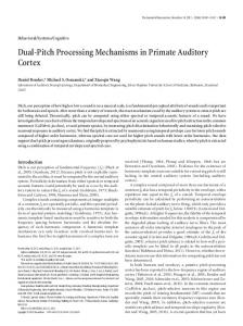
broader carrier spectrum would elicit responses from a wider signal path, eliciting more spikes, and, consequently, a wider distribution in the MPH. As Figure 2 indicates, we also observed more radical differences in the responses to SAM with tonal versus noise carriers. In this case, the BMF for rate (rBMF) is similar across carrier types (i.e., 96 Hz) but the rMTF for tonal SAM is much more sharply tuned. The tsMTFs indicate that the distribution of spike times within the modulation period were highly consistent from trial to trial for both carrier types. Figure 3 shows results from a neuron that exhibited a particularly high spontaneous rate. Tonal SAM suppressed activity quite effectively at all but the very lowest modulation frequencies, unlike noise SAM, which was associated with high firing rates and even a brief period of suppression at the end of each trial. The rMTFs, vsMTFs, and tsMTFs for this cell are very different (Fig. 3c). For example, the synchrony cutoff for tonal SAM was 24 Hz, compared with 128 Hz for noise SAM. Figure 4 shows the responses of another example neuron. In this case, the rMTF was poorly tuned for both tonal and noise SAM, and the large error bars indicate that trial to trial variability in firing rate was relatively high. However, the temporal precision of the responses to noise SAM was very high, as is evident from both the rasters and the temporal MTFs below. In fact, this cell exhibited significant synchrony at 512 Hz for noise SAM. Collectively, these four examples indicate that the response patterns of cortical neurons can vary substantially from one neuron to another, and, for a given neuron, from one carrier to another. (2) Across the population, we found that changing the spectral distribution of the carrier of SAM signals resulted in significantly ( p ⬍ 0.001) different rMTFs in 81% of cortical neurons. The significance of these changes was assessed by using permutation tests that compared the differences between the actual MTFs against the differences between simulated MTFs constructed from mixtures of the trials from each carrier type (see Materials and Methods). It is possible that some of these changes reflect rescaling of the response rates, rather than changes in modulation frequency tuning. When we performed a similar analysis after normalizing each rMTF by the total firing rate, 48% of the tonal rMTFs remained significantly ( p ⬍ 0.001) different from the rMTF obtained with the noise carrier. This result indicates that the effect of changing the carrier type did not simply rescale the response rate, but resulted in changes in modulation frequency tuning in nearly half the neurons in our sample. When we analyzed vsMTFs the same way we found that 53% of neurons exhibited significant differences ( p ⬍ 0.001) across carrier type. After normalization by the sum of the vsMTFs, the incidence of changes in tuning was 28%, indicating that changing the spectral energy distribution of the carrier changed the VS-defined modulation frequency tuning for approximately a quarter of cortical neurons. Because responses to tonal and noise SAM were obtained in consecutive runs rather than interleaved trials, we performed an additional check to ensure that the changes in the responses we observed were not due to changes in the recording conditions. We subdivided the 20 trials in each run into 10 “early” and 10 “late” trials and computed the SI (see Materials and Methods) between MTFs based on (1) the late trials from the first recorded run with the early trials from the second run, which were recorded consecutively, and (2) the early trials from the first run and the late trials from the second, which were separated by a recording time of ⬃13 min. Median values for the SIs did not differ significantly (0.68 vs 0.69; p ⬎ 0.16), indicating that


9436 • J. Neurosci., May 29, 2013 • 33(22):9431–9450

tonal carrier 512 384 256 192 128 96 64 48 32 24 16 10 8 6 4 0

noise carrier

b Modulation Frequency (Hz)

Modulation Frequency (Hz)

a

500

1000

512 384 256 192 128 96 64 48 32 24 16 10 8 6 4 0

1500

500

time (ms) 1 noise carrier

100 80 60 40

tonal carrier

20

SI: 0.73 (0.83)

1

SI: 0.48 (0.64)

0.8

Trial Similarity

140 120

0.6 0.4

8

16 32 64 128 256 512


0.6 SI: 0.81 (0.84) 0.4

0

0 4

0.8

0.2

0.2

0

1500

time (ms)

Vector Strength

Firing Rate (Spikes/Sec)

c

1000

4

8

16 32 64 128 256 512


4

8

16 32 64 128 256 512


Figure 1. Changes in spectral density elicit diverse responses from cortical neurons. The rasters shown in a and b indicate spikes fired by a single neuron in response to SAM with tonal and noise carriers, respectively. Each tick indicates the time of the spike relative to the onset of the interval over which modulation frequency was varied (see Materials and Methods for stimulus details). Spikes beyond 1000 ms were used to estimate the spontaneous firing rate. Trials have been reordered and grouped by modulation frequency. c, MTFs for average firing rate, VS, and TS, respectively. Values for the tonal and noise carriers are shown in black and gray, respectively. Vertical ticks on the rate MTF indicate the ⫾ 2 SEM over repeated trials (n ⫽ 20). Filled circles on the VS- and TS-based MTFs indicate that the metric was statistically significant ( p ⬍ 0.001; see Materials and Methods). Vertical ticks on the VS- and TS-based MTFs indicate SDs based on the jackknife and resampling procedures described in Materials and Methods. The inset on the TS-based MTF depicts the average spike waveforms during the recordings in each stimulus block (tonal and noise). The carrier frequency was 2 kHz, and the neuron’s BF was 2.0 kHz. Values for the SI for the MTFs are indicated on each panel. The SI for the MTFs normalized by the total firing rate are included in parentheses.

changes in recording conditions were unlikely to have caused the MTF differences we observed. (3) To provide context for the magnitude of the changes in MTF scale and structure we observed across carrier types, we compared the distribution of SIs across carrier type but within the same cells to the distribution of SIs obtained when we compared MTFs for tonal SAM against MTFs for noise SAM in different cells. By doing so, we take into account the diversity of cortical MTF shapes—if cortical MTFs are highly stereotyped, for example, then the SIs for random cell pairs will be high. We generated 2000 such pairs for the benchmark SI distribution. For the rMTFs, the median SI for the across-cell benchmark was 0.57, compared with 0.71 for SIs obtained across carrier types but within the same cells. Thus, rMTFs for the same cells across carrier type were 25% more similar than for different cells (also across carrier type). However, much of this difference could reflect the fact that firing rates across cells can vary widely. We recomputed the SI distributions after first normalizing the

rMTFs by their sum to eliminate differences in rMTF scale while preserving differences in rMTF shape. After this procedure, the median SI for different carrier types but the same cells was only 3% larger than the median SI for the across-cell benchmark (0.80/ 0.78). This means that the shape of the rMTF across carrier type is not much better conserved within an individual cortical neuron. We performed a similar analysis on the vsMTFs and obtained similar results. Before normalization, the median SI for the data exceeded the median benchmark SI by ⬍9% (0.67/0.62); after normalization, it exceeded it by ⬍3% (0.74/0.72). Thus, we conclude that, for a given neuron, the changes in MTF structure caused by changes in the carrier type were substantial and similar to the differences observed across cells, given the diversity of cortical MTFs. (4) The changes in MTF structure for different carrier types also suggest that instead of encoding amplitude modulation generally at a given modulation frequency, many neurons encode only tonal SAM, or noise SAM. We demonstrate this in Figure 5,


J. Neurosci., May 29, 2013 • 33(22):9431–9450 • 9437

Figure 2. Example from a single cortical neuron in response to SAM with tonal and noise carriers. Figure conventions are identical to those in Figure 1. The carrier frequency was 3 kHz, and the neuron’s BF was 3.6 kHz.

which shows the distribution of TS values for all neurons (each point represents a single modulation frequency; n ⫽ 7640). These data have been color coded to indicate whether the value for TS was significant ( p ⬍ 0.001) for both tonal and noise SAM (blue), for only tonal SAM (green), for only noise SAM (red), or for neither stimulus (gray). Most responses are not significant for either carrier type (71.4%), reflecting the fact that we tested modulation frequencies well above the synchronization limits of most cortical neurons (ⱖ96 Hz). The crucial observation is the fact that significant TS values for both carriers (8.8%) were slightly less common than significant TS values only for tonal SAM (10.7%), or only for noise SAM (9.2.%). This finding demonstrates that it is often not possible to define a neuron as robustly encoding a given modulation frequency without also specifying the carrier spectrum. Changes in carrier type produce relatively minor changes in the population representation of sound envelopes In the previous section, we described the effects of changing carrier type on the response properties of individual neurons. As we showed in Figures 1– 4, these changes varied considerably from

neuron to neuron. In this section, we attempt to characterize the population effect, on average, of changing carrier type for SAM signals. We consider (1) the effects of changing the carrier type on two common summary measures of temporal tuning, the BMF, and the synchrony (similarity) cutoffs and we then examine (2) how broadening the carrier spectrum affects the average differences between MTFs. (1) We identified the BMF for rate, VS, and TS for all neurons in the sample for each carrier type (Fig. 6; see Materials and Methods). Because we required that the firing rate at the BMF be significantly larger than the lowest recorded rate, many neurons were considered not to have a BMF (154 for tonal SAM, and 244 for noise SAM). The top row and left column are set apart to indicate that the BMF was not considered significant for at least one carrier type. The rBMFs for tonal and noise SAM differed significantly ( p ⬍ 10 ⫺6; two-sample Kolmogorov–Smirnov (KS) test), in part due to the higher incidence of significant rate tuning for tonal SAM. When we excluded nonsignificant cases from the analysis, the distributions remained significantly different ( p ⬍ 0.0066), reflecting a slight bias in favor of higher modulation frequencies


9438 • J. Neurosci., May 29, 2013 • 33(22):9431–9450

a

b


512 384 256 192 128 96 64 48 32 24 16 10 8 6 4 0

500

1500

512 384 256 192 128 96 64 48 32 24 16 10 8 6 4 0

500

60

noise carrier

50 40 30 20

tonal carrier

10

1

1

0.8

0.8

0.6 0.4 0.2

0 −10

SI: 0.33 (0.74) 8

16 32 64 128 256 512


1500

SI: 0.65 (0.66)

0.6 0.4 0.2

SI: 0.61 (0.64) 0

4

1000

time (ms)

Trial Similarity

c Firing Rate (Spikes/Sec)

1000

noise carrier

time (ms)

Vector Strength


tonal carrier

0 4

8

16 32 64 128 256 512


4

8

16 32 64 128 256 512



for noise SAM. The median rBMF was 48 Hz for tonal SAM, and 64 Hz for noise SAM, but these distributions were both quite broad (Fig. 6a). Moreover, the correspondence between rBMFs for two carrier types was poor, as is evident from the weak diagonal structure in the colored matrix depicting the joint rBMFs. Overall, the marginal distributions to the top and left of the joint rBMF matrix show a slight emphasis on modulation frequencies from 16 to 96 Hz, and a lack of emphasis from 4 to 10 Hz. More importantly, the high numbers of entries in the first row and column (excluding the top corner, which indicates a lack of tuning for either carrier type) indicate that significant rate tuning for only one carrier type was common. The population distributions of BMFs based on VS and TS were quite similar across carrier type. Results for the vsBMFs and tsBMFs are shown in a similar format in Figure 6, b and c. As long as a single point on the MTF was significant, the BMF was defined as the modulation frequency where the VS or TS was maximal. By this criterion, 92 neurons could not be assigned a vsBMF (18%) for tonal SAM, and only 49 neurons (9%) could not be assigned a vsBMF for noise SAM. After excluding these nonsignificant cases, differences between the vsBMF distributions for tonal SAM and noise SAM were marginally significant at best ( p ⬍ 0.0431; two-

sample KS test). The distributions of tsBMFs (significant cases only) did not differ for tonal SAM and noise SAM ( p ⬎ 0.12; two-sample KS test). Thus, the BMF distributions for VS and TS do not show substantial changes across the population for different carrier types, despite the fact that many individual neurons do exhibit such changes (Figs. 1– 4). Correlations between the rBMFs, vsBMFs, and tsBMFs across carrier type were significant but modest. If the BMFs were consistent across carrier types, this would appear as diagonal structure in the joint BMF matrices. These relationships were not as strong as would be expected if tuning for modulation frequency were independent of the carrier type (Fig. 6c). For neurons that could be assigned a rBMF for both tonal and noise SAM, the correlation (r) was 0.23 ( p ⬍ 0.0008; n ⫽ 220). The analogous correlation for the vsBMFs was 0.18 ( p ⬍ 0.0004; n ⫽ 399, or 76% of all neurons), and that for the tsBMFs was 0.22 ( p ⬍ 0.0034; n ⫽ 174, or 33%). The cutoff values for VS and TS were more highly conserved across carrier type than the BMFs. We defined the cutoff for VS (and TS) as the highest modulation frequency associated with a significant value ( p ⬍ 0.0001) of VS (or TS). When the VS-based cutoffs for tonal SAM and noise SAM were compared for all


a

J. Neurosci., May 29, 2013 • 33(22):9431–9450 • 9439

b

512 384 256 192 128 96 64 48 32 24 16 10 8 6 4



tonal carrier

0

500

1000

1500

noise carrier 512 384 256 192 128 96 64 48 32 24 16 10 8 6 4 0

500

time (ms)

c

1

1

0.8

0.8

Trial Similarity

20

0.6

15

0

0.6

0.4

10 5

1500

noise carrier

Vector Strength

Firing Rate (Spikes/Sec)

30 25

1000

time (ms)

tonal carrier

0.2

SI: 0.81 (0.89) 4

8

16 32 64 128 256 512


0.4 0.2

SI: 0.59 (0.69) 0

4

8

16 32 64 128 256 512


SI: 0.52 (0.69) 0

4

8

16 32 64 128 256 512



neurons where a cutoff could be identified for both carriers (n ⫽ 399), the resulting correlation was highly significant (r ⫽ 0.50; p ⬍ 10 ⫺25). The correlation between the TS-based cutoffs across carrier type where both could be defined were somewhat lower (r ⫽ 0.38; p ⬍ 10 ⫺6; n ⫽ 174), but still substantially higher than the BMF correlations in the previous paragraph. This suggests that the mechanisms that determine the upper limits on modulating encoding are less affected by changes in the carrier type than those that determine the BMF. Figure 7 shows the percentage of neurons whose responses produced significant values of VS and TS at each modulation frequency. The distributions for tonal SAM (black) and noise SAM (gray) cutoffs are quite similar. When only MTFs that include at least one significant value of VS are included, the distributions of cutoff values do not differ ( p ⬎ 0.6; two-sample KS test) for tonal and noise SAM, and the medians are both 64 Hz. Similarly, the distributions of TS cutoffs did not differ ( p ⬎ 0.1; two-sample KS test) across carrier type when limited to MTFs with at least one significant value. The median TS cutoffs were both 32 Hz. Finally, the differences between the VS and TS curves reflect the fact that the significance criterion for TS is more conservative than the Rayleigh test used for VS.

(2) The foregoing paragraphs indicate that the distributions of summary measures like the BMF for the population show relatively minor changes across carrier types. How should we reconcile this finding with the substantial changes in the MTFs observed in many individual neurons (Figs. 1– 4)? One potential explanation is that changes in some neurons (e.g., higher rBMFs for tonal SAM) counterbalance the changes observed in others (e.g., higher BMFs for noise SAM), producing similar distributions when averaged over the population. Thus, we wished to determine the extent to which differences in the responses to tonal SAM and noise SAM were idiosyncratic or consistent in the cortical population we sampled. To investigate this issue, we subtracted the MTFs for noise SAM from the MTFs obtained with tonal SAM for each neuron, and averaged the result across the population. In the case of rMTFs, we normalized the differences in firing rate at each modulation frequency by the average of the SEs of measurement associated with the two MTFs at that modulation frequency. By normalizing the data in this way, we minimize the differences associated with high trial to trial variability, and prevent neurons with high firing rates from dominating the average. Because both the VS and TS metrics are bounded (0 to 1, and ⫺1 to 1, respec-

9440 • J. Neurosci., May 29, 2013 • 33(22):9431–9450


were nearly perfectly balanced for TS, resulting in a mean of 0, and a median no different from 0 ( p ⬎ 0.4; Wilcoxon signed rank). VS was slightly but significantly ( p ⬍ 0.001; Wilcoxon signed rank) higher for tonal SAM than for noise SAM at a limited number of modulation frequencies, as indicated by the filled circles on the vsMTF difference curve (gray). For tsMTFs, however, the median difference was significantly different from zero only at 4 Hz, in favor of noise SAM, and all TS values showed less of a tonal advantage than did the values for VS. It is important to recall that VS measures the concentration of spikes at a particularly phase of the modulation period, while TS simply measures the trial to trial variability in spike phase. Thus, the cortical population appears to represent modulation frequencies with approximately equal temporal fidelity overall, despite the fact that individual neurons often encode different carrier types quite differently (Fig. 5).

Figure 5. Cortical neurons more commonly exhibited significant values of TS for only a single carrier class than for both classes. Each circle on the scatterplot corresponds to a pair of TS values (one for tonal SAM, one for noise SAM) for a single neuron and modulation frequency. The unity line and a box indicating the location of (0,0) are added for convenience. Color coding indicates whether statistical significance ( p ⬍ 0.001) was achieved for the pair of TS values, with gray for neither class, red for noise SAM only, green for tonal SAM only, and blue for both.

tively), we used the raw data when generating average differences for the vsMTFs and tsMTFs. Firing rates for noise SAM were significantly ( p ⬍ 0.001) higher on average than those for tonal SAM throughout the tested range of modulation frequency, particularly at the highest modulation rates (Fig. 8a). For firing rate, then, there appears to be a consistent trend in favor of higher response rates for noise SAM relative to tonal SAM. The histogram to the right of Figure 8a shows the normalized firing rate differences for all points on the MTF difference functions for all neurons. The distribution is significantly (Wilcoxon signed rank; p ⬍ 10 ⫺145) shifted to the left of 0 (indicated by the gray line), resulting in a mean of ⫺1.39 ⫾ 5.20. However, there were clearly many cases (36%) where the responses to tonal SAM at a given modulation frequency exceeded those to noise. The high SD indicates that fairly large rMTF differences were common, as demonstrated in the previous section. Thus, it appears that while there is a general trend for higher firing rates to noise SAM, this trend reflects imperfect “balancing” of large, idiosyncratic changes in individual cortical neurons, rather than minor changes that favor noise SAM in most neurons. We found a slight but significant bias in favor of higher VS values for tonal SAM (mean: 0.04; p ⬍ 10 ⫺57; Wilcoxon signed rank) relative to noise SAM (Fig. 8b; gray curve). As was true for the rMTFs, this bias reflected an imperfect balancing of substantial but heterogeneous changes in different neurons. For the tsMTFs (Fig. 8b; black curve), we found that the distribution of tsMTF differences was even wider than for the rMTFs and vsMTFs, as indicated by the histograms to the right of Figure 8. The changes produced by exchanging tonal SAM for noise SAM

Modulation frequency encoding is dominated by spike timing information for both tested carrier types In this section, we use spike train classification techniques to characterize how information about modulation frequency is represented in the spiking patterns of cortical neurons. These techniques allow us to parse the contribution of firing rate differences across modulation frequency from the contribution of differences in temporal spiking patterns. As in prior reports (Malone et al., 2007, 2010), we computed Confusion matrices for three distinct classifier types (see Materials and Methods). The first uses the full spike train; the second “phase-only” classifier uses rate-normalized timing information; the third “rate-only” classifier relies on the firing rate averaged over the duration of each trial. We compute discrimination performance as the percentage of trials in which the correct modulation frequency was identified based on the response in that trial. Spike timing information was far more effective for discriminating modulation frequency than average spike rate for both noise and tonal carriers, as indicated by Figure 9, which plots the performance of the phase-only and rate-only classifiers against performance for the full spike train classifier. Performance for the phase-only classifier (black circles) nearly matched that of the full spike train classifier, unlike performance for the rate-only classifier (gray circles). As a result, the discrepancy between the phaseonly and rate-only classifiers was very highly correlated with discrimination performance for the full spike train classifier for tonal SAM (r ⫽ 0.91; p ⬍ 10 ⫺197) and noise SAM (r ⫽ 0.90; p ⬍ 10 ⫺184). In fact, cortical discrimination of modulation frequency was often near chance levels when timing information was omitted. Median discrimination performance for the full spike train classifier was slightly but significantly higher than that based only on response phase for tonal SAM (17.3 vs 16.0%; p ⬍ 0.0044; Fig. 9a). Median performance for the rate-only classifier was significantly lower (10.7%; p ⬍ 10 ⫺42). Results were similar for noise SAM—median performance for the full spike train classifier (14.3%) was marginally better than that of the phase-only classifier (14.3 vs 14.0%; p ⫽ 0.0226). Again, the performance median for the rate-only classifier was significantly lower (9.3%; p ⬍ 10 ⫺64). These findings underscore the relative importance of spike timing and the close similarity between cortical SAM processing in squirrel monkeys and macaques in this regard (Malone et al., 2007, 2010). The foregoing results also indicate that median performance was better for tonal SAM than for noise SAM. Although the differences are relatively small, they were significant for the full spike


J. Neurosci., May 29, 2013 • 33(22):9431–9450 • 9441

Neurons (%) with Significant VS/TS

100 90 80 70 60 50

VS (noise) VS (tonal)

40 30 20

TS (noise) TS (tonal)

10 0

4

6

8 10 16 24 32 48 64 96 128

256

512

Modulation Frequency (Hz) Figure 7. The incidence of significant synchrony (VS) and similarity (TS) was relatively high in our sample, and persisted to relatively high (⬎64 Hz) values for a substantial minority of neurons. Curves indicate the percentage of neurons exhibiting significant VS/TS at the modulation frequency along the abscissa (gray, noise carriers; black, tonal carriers).

train (17.3 vs 14.3%; p ⬍ 10 ⫺6), phase-only (16.0 vs 14.0%; p ⫽ 0.0011), and rate-only (10.7 vs 9.3%; p ⬍ 10 ⫺10) classifiers. These results confirm that although changes in carrier type profoundly affect the responses of individual neurons, across the population the quality of the encoding of tonal and noise SAM is relatively similar. However, we also observed that as discrimination performance across both carrier types increased, the difference between performance for tonal and noise SAM also increased (r ⫽ 0.29; p ⬍ 10 ⫺10). This indicates that not only is there a genuine processing advantage for tonal SAM, but that this advantage is largest among the neurons that encode modulation frequency most effectively. Maximum firing rate is positively correlated with modulation frequency discrimination performance In this section, we characterize the relationship between overall firing rate and temporal discrimination in cortical neurons. We characterized the relationship between maximum firing rate and discrimination performance by correlating percentage correct for each classifier with the maximum average firing rate elicited at the rBMF for each MTF. These correlations were robust for tonal SAM, particularly for the full spike train (r ⫽ 0.68; p ⬍ 10 ⫺70) and phase-only (r ⫽ 0.67; p ⬍ 10 ⫺66) classifiers, and somewhat less so for the rate-only classifier (r ⫽ 0.50; p ⬍ 10 ⫺33). This pattern held for noise SAM as well, but the discrepancy between the rate-only classifier (r ⫽ 0.30; p ⬍ 10 ⫺11) and both the full spike train (r ⫽ 0.58; p ⬍ 10 ⫺47) and phase-only classifiers (r ⫽ 0.58; p ⬍ 10 ⫺47) was larger. For the rate classifier, the more directly relevant measure is the difference between the maximum Figure 6. BMFs defined in terms of either rate, VS, or TS differed substantially across MTFs obtained for tonal and noise carriers. Histograms summarizing the marginal distributions are shown above and to the left of the joint distribution matrices. Colors indicate cell counts from zero (dark blue) to the maximum (dark red). A white X in the top left corner of the matrix (a and c) indicates that the axis was broken because the BMF could not be defined for either carrier in many cases (n ⫽ 95 in a; n ⫽ 162 in c). The matrix was rescaled to the next highest entry to avoid compression of the values other than the maximum. Color bars indicate the cell counts for the rescaled axes. Broken histogram bars are used to indicate that the histogram bar was not

4 plotted to scale due to the high incidence of MTFs with no significant BMF for rate (a; see Materials and Methods), or MTFs that lacked at least one significant ( p ⬍ 0.001) value of VS (b) or TS (c). The white rectangles enclosing the top row and left column of each matrix indicate that a BMF could not be assigned because the firing rates did not differ significantly (for rMTFs), the responses were unsynchronized (for vsMTFs), or the responses were not significantly reproducible from trial to trial (for tsMTFs).

9442 • J. Neurosci., May 29, 2013 • 33(22):9431–9450


Figure 8. On average, broadening the carrier spectrum resulted in significantly higher firing rates across the tested range of modulation frequencies, but had a modest impact on VS and little effect on TS. The curves in both a and b show the mean differences between the tonal and noise MTFs as a function of modulation frequency. a, The rMTF for noise was subtracted from the rMTF for tones, and normalized by the average of the SE of measurements obtained for each MTF. Circles on individual points indicate that the median value for the difference between tonal SAM and noise SAM responses was significantly ( p ⬍ 0.0001) different from 0 (Wilcoxon signed rank). The histogram to the right shows the normalized differences between all pairs (Figure legend continues.)


J. Neurosci., May 29, 2013 • 33(22):9431–9450 • 9443

a

b 0.8

tonal SAM

Percent Correct: Phase and Rate

Percent Correct: Phase and Rate

0.8

0.6

0.4

0.2

noise SAM

0.6

0.4

0.2

0

0 0

0.2

0.4

0.6

0.8

Percent Correct: Full Spike Train

0

0.2

0.4

0.6

0.8

Percent Correct: Full Spike Train

Figure 9. Cortical discrimination of modulation frequency is dominated by spike timing information. a, Discrimination performance based on the full spike train (abscissa) is compared against performance based only on phase (black circles) and average rate (gray circles) for tonal carriers. Values along the diagonal indicate equivalent performance. b, Similar comparisons are plotted for data obtained with noise carriers. All data are based on the optimal binwidth for each neuron, stimulus type, and classifier.

and minimum values in each MTF, because it is possible that all rMTF values could approximate the maximum value (i.e., for a flat rMTF). However, the span of rates is very highly correlated with the maximum rate across our sample of MTFs (r ⬎ 0.90 for both carrier types). Nevertheless, the correlations between the span and rate-only classifier performance do improve (tonal SAM: r ⫽ 0.56, p ⬍ 10 ⫺68; noise SAM: r ⫽ 0.43, p ⬍ 10 ⫺24), while the correlations between discrimination performance and the rate span for the other classifiers are essentially the same as the correlations with maximum firing rate. The essential point is that higher firing rates are universally associated with better discrimination performance, even when differences in average firing rate across stimuli are eliminated by normalization (i.e., for the phase-only classifier). To understand why more spikes are associated with better modulation frequency discrimination, it is important to be clear that what we mean by “spike timing information,” in the context of spike train classification, is related to the resolution at which we measure changes in firing rate. As we noted in Materials and Methods, increasing the resolution of the classifier (i.e., using more and smaller bins in the PSTH) will only improve performance if the timing of the spikes produced by the neuron is similarly precise. That is why our estimate of the size of the temporal integration window for each neuron is obtained by calculating the binwidth that optimizes modulation discrimination performance. Figure 10 shows the histograms of the optimal bin4 (Figurelegendcontinued.) ofpointsontherMTFs,forallneurons.Thegraylineindicateszero,and the flanking white lines indicate the limits of the ordinal axis in the panel to the left. Details of the distribution are as follows: mean: ⫺1.39; SD: 5.20; skewness: 0.21; kurtosis: 5.76. b, Graphical conventions are the same as in a. The vsMTFs and tsMTFs were not normalized because the metrics themselves are bounded. Details of the distribution of vsMTF differences are as follows: mean: 0.04; SD: 0.22; skewness: 0.18; kurtosis: 4.80. For tsMTF differences: mean: 0.00; SD: 0.27; skewness: ⫺0.03; kurtosis: 3.57.

Figure 10. The typical temporal resolution of cortical neurons is ⬃10 ms. This pair of histograms summarizes the distributions of optimal binwidths used for the discrimination of modulation frequency by the full spike train classifier across all neurons in our database.

width for each neuron for each carrier type. Only those cells whose overall performance, expressed as a z-score, exceed 3 SDs relative to the simulated matrices used for significance testing (see Materials and Methods) are included. The distributions are broad, and fairly similar, although the distribution for noise SAM is more focused around 8 and 10 ms, while that for tonal SAM has more entries at both 4 and 20 ms (␹ 2 test; p ⫽ 0.0381). Since neurons that can fire at higher rates have a larger effective dynamic range for a given temporal interval (e.g., one neuron might fire between 0 and 10 spikes in a 20 ms bin, while another can only fire between 0 and 5 spikes), this may explain why neurons with higher maximum firing rates are generally better at discriminating modulation frequency. We also verified that the correlations between maximum firing rate and classifier performance were not based on a categorical distinction between cells that did not respond to or encode SAM, and cells that did. We converted classifier performance into

9444 • J. Neurosci., May 29, 2013 • 33(22):9431–9450


Figure 11. The confusion matrices in a and b depict the success rate of the full spike train classifier in identifying the modulation frequency based on the spike trains elicited by tonal SAM and noise SAM, respectively. Responses along the diagonal represent correct identification, when the estimate of the modulation frequency for a given trial matched the actual modulation frequency presented on that trial. The “heat” of each element of the matrix (from blue to red) indicates the number of trials that were mapped to that element. The percentage values in the upper right corner of each matrix indicate the percentage correct across all trials and stimuli. These data correspond to the example responses shown in Figure 1, and represent good discrimination performance relative to the cortical population. c, The CCM shows the performance of the full spike train classifier when trials obtained during presentation of both tonal and noise SAM were combined. The concentration of values along the main diagonal, and near absence of values along the “minor” diagonals in the bottom left and top right quadrants, indicate that responses to tonal and noise SAM at the same modulation frequencies were sufficiently distinct to be discriminated from one another.

z-scores (see Materials and Methods), limited the data to cases where z ⬎ 3, and recomputed the correlations between classifier performance and maximum firing rate. Reductions in the correlation coefficients were modest, averaging 0.05, and never exceeding 0.07. For example, the correlation for the full spike train classifier for tonal SAM was reduced from 0.68 to 0.65. The strong correlation between maximum firing rate and modulation frequency discrimination performance suggests that one could predict whether discrimination is better for tonal SAM or noise SAM by knowing which carrier type elicits a higher maximum rate from a given neuron. As expected, the logarithm of the ratio of the maximum firing rate associated with the tonal and noise MTFs was significantly predictive of the performance differential across carrier types for all classifiers (r ⬎ 0.47; p ⬍ 10 ⫺30 for all three correlations). We also identified an interesting asymmetry in this relationship. We classified neurons that exhibited the highest firing rate for a tonal carrier as “tone-preferring” (n ⫽ 240) and the remainder as “noise-preferring” (n ⫽ 283). Among tone-preferring neurons the performance advantage enjoyed by tonal carriers was substantial (22.3 vs 13.7%; p ⬍ 10 ⫺20). Among noise-preferring neurons, however, the slight advantage for noise carriers was marginal (14.6% vs 15.3%; p ⫽ 0.0225). Analogous results were obtained with the phase-only and rate classifiers. Thus, while neurons that are driven most effectively by tonal carriers discriminate modulation frequency better for tonal carriers than for noise carriers, the reverse is not true to the same extent. This suggests that the “additional” spikes (relative to the tonal MTF) fired by noise-preferring neurons do not contribute to the discrimination of envelope periodicity as effectively, and reinforces the notion that there is a genuine temporal processing advantage for narrowband signals. Interestingly, overall responsiveness seems to be more highly conserved across carrier type than the quality of the representation of modulation frequency. The correlation between maximum driven rates across carrier types was strong (r ⫽ 0.64; p ⬍ 10 ⫺60), and even stronger when firing rates summed across the MTF were used (r ⫽ 0.72; p ⬍ 10 ⫺83). However, the correla-

tion between discrimination performance for the two carrier types (based on the full spike train classifier) is weaker (r ⫽ 0.46; p ⬍ 10 ⫺27) than either the correlation between maximum rate and performance, or the correlation between maximum rate across carrier types (see above). Both modulation frequency and carrier type can be effectively discriminated by the information in cortical spike trains In this section we quantify the ability of cortical neurons to discriminate carrier type. In previous sections we characterized the ways in which changing carrier type changed cortical MTFs. Here, we use spike train classification techniques to quantify the information inherent in the underlying, trial by trial changes in spiking patterns. To test whether carrier type could be distinguished based on cortical spike trains, we constructed CCMs by combining responses to tonal and noise SAM. Confusion matrices for tonal SAM, noise SAM, and the CCM for a single neuron are shown in Figure 11 (these matrices are based on the same responses as Fig. 1). Discrimination performance for this neuron was among the best observed in the data sample. For tonal SAM (Fig. 11a), discrimination was very nearly perfect for values ⬍64 Hz, the range corresponding to the plateau in TS (Fig. 1c), so nearly all entries appear on the diagonal (i.e., the modulation frequency estimated by the classifier matched the actual frequency). For noise SAM, performance was much lower overall (45 vs 71%), though still far above chance performance (6.7%). For CCMs, we define correct responses as cases where both the modulation frequency and the carrier type were estimated correctly. This is because errors can occur not only when the response for a given trial is associated with the incorrect modulation frequency, but also when the response is associated with the correct modulation frequency but with the incorrect carrier type. We refer to the latter as “carrier confusion errors.” For the data shown in Figure 11c, however, carrier confusion errors almost never occurred - the CCM is very much like the confusion matrices in Figure 11, a and b, arranged corner to corner along the diagonal, with very few entries in either the bottom left or upper right quadrants of the CCM. This


J. Neurosci., May 29, 2013 • 33(22):9431–9450 • 9445

confusion errors (r ⫽ 0.89; p ⬍ 10 ⫺177). This result indicates that spike timing information supports both modulation frequency and carrier-type discrimination. Interestingly, however, the correlation between phase-only and rate-only classifier performance was also significant (r ⫽ 0.47; p ⬍ 10 ⫺29), which implies that the quality of spike timing and average rate information are related.

Figure 12. The scatterplot compares percentage correct for the CCMs against the incidence of carrier confusion errors. For CCMs, carrier confusion errors are defined as cases where the classifier estimate of the modulation frequency is correct, but the estimate of the carrier type for the trial is incorrect. Correct responses (x-axis) mean that both modulation frequency and carrier type were successfully estimated. Results for the full spike train classifier, phase-only, and rate-only classifiers are shown in black, dark gray, and gray circles, respectively, as indicated by the legend.

means that the responses of this neuron contained enough information to discriminate modulation frequency and carrier type in tandem. The incidence of carrier confusion errors across the population was near chance levels. Chance predicts a carrier confusion error rate of 3.33% (100/30) for a CCM based on 15 distinct modulation frequencies (the typical number used in these experiments). The median percentages of carrier confusion errors for the full spike train, phase-only, and rate-only classifiers were 3.5, 3.8, and 3.0%, respectively, compared with medians for correct responses (i.e., correct identification of both modulation frequency and carrier type) of 11.7, 10.2, and 5.9%. Figure 12 shows the comparison between the percentage correct and the percentage of carrier confusion errors for each of the classifiers and for all neurons in the population. If cortical response supported the discrimination of modulation frequency, but not carrier type, then all points would lie along the diagonal. As is evident from Figure 12, the correlation between percentage correct and the percentage of carrier confusion errors was significantly positive for the full spike train (r ⫽ 0.40; p ⬍ 10 ⫺20) and phase-only (r ⫽ 0.51; p ⬍ 10 ⫺34) classifiers. This result is to be expected since carrier confusion errors require correct identification of the modulation frequency, and we presented far more distinct modulation frequencies than carrier types (i.e., 15 vs 2). The analogous correlation for the rate-only classifier was weak and even slightly negative (r ⫽ ⫺0.10; p ⫽ 0.0206), likely because performance based on average rate information was poor. The fact that the error rates were low relative to the percentage correct indicates that the spectral characteristics of SAM stimuli are also represented in cortical firing patterns. Discrimination performance for the CCMs was almost perfectly correlated between the full spike train and phase classifiers (Fig. 12; r ⫽ 0.98; p ⬍ 10 ⫺178), as was the incidence of carrier

Spike timing and average rate information contribute to carrier-type discrimination differently at different modulation frequency ranges We directly examined how well cortical spike trains could be used to discriminate the carrier type by constructing sets of 2 by 2 confusion matrices at each tested modulation frequency. Figure 13 shows carrier discrimination performance as a function of modulation frequency. Because only responses to the same modulation frequency are classified, the percentage correct expected by chance for two carrier types is 50%. Each point on Figure 13a represents the population-averaged percentage correct as a function of modulation frequency. The divergent slopes for the phase-only (green curve) and rate-only (red curve) classifier indicate that spike timing and average rate information contribute to carrier-type discrimination in a frequency-dependent manner. Specifically, the phase-only classifier outperforms the rate-only classifier by the largest margins at the lowest modulation frequencies (⬍64 Hz). Carrier discrimination for the full spike train classifier (blue curve), which combines spike timing and average firing rate information, is comparatively flat. The similarity between the full spike train and phase-only curves from 4 to 16 Hz suggests that timing information is sufficient to support carrier discrimination at the range of modulation frequencies most important for human speech and primate vocalizations. A similar pattern is evident when the percentages of neurons, which exhibited carrier discrimination that significantly exceeded chance ( p ⬍ 0.001), are plotted as a function of modulation frequency for each of the classifiers (Fig. 13b). The fact that the incidence of significant performance for the rate-only classifier increases with modulation frequency suggests that rate information is of particular value at the high end of the tested range. Few cortical neurons evince robust average firing rate coding of modulation frequency in the absence of temporal synchrony to the stimulus envelope In this section we evaluate the notion that there exist discrete populations of neurons that employ distinct codes to represent temporal modulations in acoustic signals (Lu et al., 2001; Malone et al., 2007; Wang et al., 2012). Some neurons in marmoset auditory cortex were observed to synchronize to SAM signals, while others, the “nonsynchronized” population, exhibited significant changes in firing rate across modulation frequency in the absence of temporal synchrony to the modulation. This issue was recently addressed by Yin et al. (2011), who calculated the percentages of synchronized, nonsynchronized, and “mixed-mode” neurons, which exhibited firing rate changes above their own synchrony cutoffs, as was reported previously in macaques (Malone et al., 2007). Importantly, Yin et al. (2011) used noise carriers, while previous studies used tonal carriers. Because we presented both tonal and noise carriers in this study, our results are uniquely situated to resolve discrepancies on this point. Most neurons in our sample exhibited significant ( p ⬍ 0.001) synchrony to at least one modulation frequency. We tallied the percentage of vsMTFs that included at least one, two, or three significant VS values using the Rayleigh criterion. We report


9446 • J. Neurosci., May 29, 2013 • 33(22):9431–9450

Percent of Neurons (%)

Percent Correct %)

the incidence of synchrony for multiple a b points within each MTF because of con85 50 cerns raised about the sensitivity of Ray45 leigh statistics (Yin et al., 2011). Results of 80 this analysis are compiled in Table 1, 40 which demonstrates that synchrony to enfull spike train velope modulations was prevalent for 75 35 both carrier types. Given the high incidence of synchrony, 30 70 phase-only robust average rate coding in the absence 25 of synchrony was necessarily rare. Table 2 65 shows the percentages of rMTFs that ex20 hibited significant variation in firing rate rate-only across modulation frequency ( p ⬍ 0.001; 60 4 8 16 32 64 128 256 512 4 8 16 32 64 128 256 512 Wilcoxon rank sum). Comparison of the Modulation Frequency (Hz) Modulation Frequency (Hz) first columns of Tables 1 and 2 reveals that significant rate tuning was less common Figure 13. The relative contributions of spike rate and timing information to the discrimination of carrier type vary as a function than significant temporal synchrony of modulation frequency. Chance performance for the carrier discrimination task is 50%. a, The curves show the populationoverall, particularly for noise SAM. The averaged percentage correct for the full spike train (blue), phase-only (green), and rate-only (red) classifiers. Vertical lines indisecond column of Table 2 indicates the per- cate ⫾ 2 SEM. b, Each curve indicates the percentage of neurons in the database that single-trial responses could be used to centages of mixed-mode responses, defined identify the carrier type at a rate significantly ( p ⬍ 0.001) above chance for each classifier type. by significant rate variation for modulation frequencies above the synchronization limit Table 1. The table shows the percentage of neurons in the population with a vsMTF of the vsMTF. The fact that mixed-mode responses were more comcontaining one or more (left column), two or more (middle column), or three or mon for tonal SAM than for noise SAM, in the same population of more (right column) significant points neurons, indicates that it is more appropriate to classify the reNumber of significant values on the vsMTF ( p ⬍ 0.001) sponses rather than the neurons as mixed-mode. Finally, the third 1 or more 2 or more 3 or more column of Table 2 shows how often significant rate tuning coincided with a complete absence of temporal synchrony. Neurons that exTonal SAM 82.4% 72.4% 65.4% Noise SAM 90.6% 80.1% 73.0% hibited neither synchrony nor firing rate modulation for either carBoth carrier types 76.3% 62.1% 53.2% rier were rare (1.1%), but still slightly more common than neurons Neither carrier type 3.2% 9.4% 14.7% that used a completely nonsynchronized rate code across carrier type The rows specify the carrier type category (tonal, noise, both, or neither). The categories are not exclusive, so (1.0%). a neuron with exactly two significant points in the tonal vsMTF and two in the noise vsMTF will be counted We also checked whether larger changes in firing rate were assoamong all six percentages in the top three rows of the two leftmost columns. The same neuron will also be counted in the last row, right column, because neither the tonal vsMTF nor the noise vsMTF contains three or ciated with the range of modulation frequencies beyond the synmore significant points. chrony cutoffs of each neuron. To do so, we computed the “rate span” by subtracting the minimum rate from the maximum rate. Table 2. The percentages of neurons in the population with significant firing rate tuning We then calculated the portion of the rate span occurring below and above the synchrony cutoff. For tonal SAM, the median percentage Incidence of significant firing rate tuning ( p ⬍ 0.001) of the total rate span within the synchronized range was 73%, comAll Above the vsMTF cutoff AND no vsMTF synchrony pared with 63% above the cutoff. This difference was marginally Tonal SAM 70.6% 37.1% 7.6% significant (p ⫽ 0.0457). For noise SAM, the analogous percentages Noise SAM 53.4% 21.4% 4.0% were 75.0 and 65.9% (p ⬍ 0.0002). These results contradict the Both carrier types 42.1% 10.7% 1.0% notion that average firing rate differences occur chiefly in the modNeither carrier type 18.2% 52.2% 1.1% ulation frequency range where timing information is no longer The rows specify the carrier type category (tonal, noise, both, or neither), as in Table 1. The leftmost column specifies available due to limits in response synchronization. Of course, in that all points in the vsMTF are considered. The middle column specifies that only modulation frequencies above the neuron’s synchronization cutoff are considered. The right column represents a logical AND, such that a neuron must cells where the synchrony cutoff is higher, a larger proportion of the exhibit significant firing rate tuning in the absence of temporal synchrony to qualify. Thus, 7.6% of all cells exhibited MTF will fall below the cutoff, which would tend to increase the unsynchronized rate tuning for tonal SAM (as opposed to 7.6% of neurons with nonsignificant vsMTFs exhibited fraction of the rate span in the synchronized range. Thus, while significant rate tuning). Significant firing rate tuning was defined by a significant difference in firing rate between at least two points in the rMTF (see Materials and Methods). our data do not suggest that rate coding is preferentially associated with the synchronized range, the data do demonstrate that given the prevalence of cortical synchrony, more of the total variwithin a two-octave range, a small discrepancy between the BF ation in average firing rate occurs in the synchronized range of and the chosen carrier (i.e., ⬍2 octaves) would not prevent the modulation frequency. carrier of noise SAM from overlapping the receptive field of the neuron. For tonal SAM, however, a mismatch between the Mismatches between the carrier frequency and BF do not carrier and the BF might be expected to have a larger effect explain the differences in the responses to tonal SAM and since the stimulus spectrum (including the sidebands at the noise SAM carrier ⫾ modulation frequency) might not overlap the recepThe difference in the spectral density of the stimuli used in tive field. For nearly all penetrations, we found that BFs for the these experiments suggests that misalignment of the carrier deeper channels increased relative to the shallower channels. frequency and the BF of a given neuron would affect responses Because we used linear probes for simultaneous recordings, to tonal SAM differently than responses to noise SAM. Behowever, it was necessary to select a single carrier frequency, cause the carrier spectrum for noise SAM is effectively flat resulting in relative differences between the carrier frequen-


J. Neurosci., May 29, 2013 • 33(22):9431–9450 • 9447

Figure 14. Misalignment of the carrier frequency and the recording channel BF does not explain the observed preferences for tonal versus noise carriers in our data sample. a, The scatterplot shows the discrimination performance of the full spike train classifier for tonal and noise SAM color coded by the octave difference between the channel BF and carrier frequency (CF). Points will fall along the unity line when discrimination of modulation frequency is equivalent across carrier types. b, The curve indicates the mean difference in TS across carrier types as a function of the octave difference between the channel BF and carrier frequency. Vertical lines indicate ⫾ 2 SEM.

cies and BFs at different recording depths. We investigated the extent to which such differences could explain the carrier preferences expressed by cortical neurons. Differences between the carrier frequencies and the channel BFs had relatively little impact on our results. First, it should be noted that most neurons were tested near their BFs; ⬎80% of the channel BFs were within a half-octave of the SAM carrier frequency. We defined the carrier mismatch as the absolute value of the ratio of the channel BF and carrier frequency in octaves. There was no relationship between the carrier mismatch and the logarithm of the ratio of the maximum firing rates obtained for tonal SAM and noise SAM (r ⫽ 0.01; p ⬎ 0.8), nor was there a relationship between the carrier mismatch and the logarithm of the ratio of the firing rates summed across the rMTFs (r ⫽ ⫺0.01; p ⬎ 0.8). We also calculated the correlation between the carrier mismatches and discrimination performance for carrier type. Differences in response rate across carrier types will support improved discrimination between them when they are compared at equivalent modulation frequencies. We found a trend suggesting that as the carrier mismatch increased, tonal and noise SAM were discriminated more effectively by the full spike train classifier (r ⫽ 0.11; p ⬍ 0.02). Importantly, however, this trend held for the phase-only classifier (r ⫽ 0.12; p ⬍ 0.02), but not for the rate-only classifier (r ⫽ 0.06; p ⬎ 0.3). This contradicts the notion that differences in average firing rate support better discrimination for larger carrier mismatches. Further, there was no significant correlation between the modulation frequency discrimination performance of the full spike train (r ⫽ 0.03; p ⬎ 0.56), phaseonly (r ⫽ 0.03; p ⬎ 0.63), or rate-only (r ⫽ ⫺0.01; p ⬎ 0.86) classifiers and the carrier mismatch, We obtained essentially identical results when we replaced the carrier mismatch with the channel depth, relative to the shallowest electrode, in the correlation against discrimination performance (r ⬍ 0.04; p ⬎ 0.49 for each of the classifiers).

We plotted discrimination performance (based on the full spike train classifier) for tonal SAM against noise SAM after color coding the data into cases where the carrier and BF mismatch was either smaller or larger than half an octave (Fig. 14a). If it were the case that large tuning mismatches resulted in better encoding of noise SAM relative to tonal SAM, then points shown in blue would lie above the unity line. Instead, the performance differences across carrier types are distributed widely both within and beyond the half-octave range. Tonal SAM was more reliably encoded than noise SAM when the channel BFs were within an octave of the carrier frequency. We documented this by computing the differences in the TS metric for all points of the MTF where the response to at least one carrier type was significant, and averaged the TS differences across the population within quarter octave ranges (Fig. 14b). It is important to note that the TS metric is an excellent predictor of discrimination performance because reflects trial to trial variability. The correlation between the sum of all TS values within each MTF (with nonsignificant values set to 0) and discrimination performance was very high for both tonal SAM (r ⫽ 0.89; p ⬍ 10 ⫺179) and noise SAM (r ⫽ 0.89; p ⬍ 10 ⫺181). In summary, we did not find compelling evidence that carrier preference was significantly related to the choice of the carrier frequency, relative to the channel BF. Instead, our results suggest that spectral density preference is relatively robust even when the tonal carrier frequency and the noise center frequency are not precisely aligned with a given neuron’s BF.

Discussion The principal finding in this study was that the spectral bandwidth of dynamic stimuli that share identical modulation waveforms and center frequencies has diverse and substantial consequences for cortical responses. The fact that cortical neurons do not represent modulation envelopes independently of the carrier bandwidth has broad implications for how complex

9448 • J. Neurosci., May 29, 2013 • 33(22):9431–9450

sounds are processed. Narrowband and relatively broadband (i.e., two-octave) carriers are expected to elicit responses from divergent populations of neurons throughout the auditory pathway. Our results suggest that the entire “effective signal pathway,” rather than a single membrane time constant local to the recorded neuron, dominates the temporal features of cortical responses. This interpretation may explain why the average correlation between tonal and noise MTFs obtained in the same neuron was approximately equivalent to the correlation between any two randomly paired MTFs in our sample. Our results complement the recent demonstration that cortical responses reflect complex interactions between spectral pattern (i.e., ripple frequency on a spectral axis) and spectral bandwidth for static stimuli (O’Connor et al., 2010). Malone et al. (2007) showed that cortical neurons encode envelope shape rather than merely extracting the periodicity of SAM signals. Analogous results have been obtained in the inferior colliculus (Krebs et al., 2008; Zheng and Escabí, 2008). Here, we show that cortical neurons also do not encode the modulation envelope independently of spectral context, and that cortical spiking dynamics are sufficiently rich to encode information about modulation frequency and carrier type simultaneously. Changing the spectral density while holding the signal energy constant will affect the “effective stimulus amplitude” delivered to neurons with narrow spectral tuning, which is relevant because changes in carrier level have previously been shown to change the shape of MTFs in the cortex (Malone et al., 2007) and inferior colliculus (Krishna and Semple, 2000). In the current study, the temporal information was identical across frequency, notwithstanding the fluctuations in signal power within narrow spectral bands endemic to noise carriers (Dau et al., 1997a; Scott et al., 2011; Fig. 11a). Thus, a change in the information conveyed about the stimulus envelope by the spike train reflects either (1) the change in the effective stimulus amplitude, given the tuning bandwidth of the neuron, or (2) a change in the quality of the temporal information conveyed to the neuron due to “cross talk” within its signal pathway. This second factor implies that two modulated signals matched in “effective” amplitude for a given neuron could still give rise to distinct response patterns because the temporal coherence among responding neurons in the signal pathway for each signal might vary (e.g., greater variance in the latency distribution). The fact that cortical neurons tended to respond quite differently to tonal and noise SAM is a challenge for linear receptive field models dominated by local spectral structure (Eggermont, 2011). Such models would predict scaling of the response magnitude for different spectral densities, but would not account for either the substantial changes in MPH shape or shifts in MTF tuning we observed in many neurons. The changes in temporal tuning we observed in many neurons indicate that the fine structure and envelope of dynamic acoustic signals interact in a complex fashion to generate cortical responses. Although responses to simple dynamic envelopes, such as those produced by SAM, have been well characterized at multiple stages of the auditory pathway (for review, see Joris et al., 2004; Malone and Schreiner, 2010), including the cortex (Creutzfeldt et al., 1980; Schreiner and Urbas, 1986, 1988; Eggermont, 1991, 1994, 1999, 2002; Langner, 1992; Gaese and Ostwald, 1995; Liang et al., 2002; Malone et al., 2007, 2010; Yin et al., 2011), few studies have described how changes in spectral bandwidth affect central auditory responses (IC: Rees and Møller, 1987; Mu¨ller-Preuss et al., 1994; thalamus: Bartlett and Wang, 2011; cortex: Bieser and Mu¨ller-Preuss, 1996; Eggermont, 2002). Eggermont (2002) re-


ported a higher incidence of synchrony, higher average peak VS, higher average firing rates, and slightly higher synchronization cutoffs for noise SAM relative to tonal SAM for the anesthetized cat. Our results differ in that we obtained the most temporally precise responses with tonal rather than noise carriers. Lu and Wang (2000; awake marmoset) reported that cortical synchronization cutoffs were fairly consistent across repetitive click stimuli with differing spectra (i.e., Gaussian vs rectangular clicks), and Bartlett and Wang (2011) obtained a similar result in a small sample of thalamic neurons tested with both tonal SAM and noise SAM at each neuron’s optimal bandwidth for static tones. The summary measures used in prior studies (e.g., synchronization cutoff, classification of MTFs as “bandpass” vs “lowpass”) do not effectively capture the discriminability of cortical spiking patterns elicited by different stimuli, however. A neuron with identical cutoff values for tonal and noise SAM could still be much more effective at encoding tonal SAM via spike timing up to that limit, for example. Our study is the first to assess changes in cortical spike timing directly, in addition to providing statistical verification for changes in MTF scale and shape. The relative utility of average firing rate information and spike “phase” information in encoding modulation frequency was highly consistent with prior data obtained in macaque monkeys (Malone et al., 2007, 2010). Moreover, our data clearly indicate that higher average firing rates are associated with better performance, even for the phase-only classifiers. This is because each spike provides an opportunity to convey additional information about the modulation envelope. Although the normalization of firing rate differences across stimuli (and modulation frequency in particular) often had relatively little impact on discrimination performance, this does not mean that average firing rate is not a crucial constraint on the representation of acoustic signals, or that average rate differences are not used. In fact, recent studies in both monkeys (Lemus et al., 2009) and cats (Dong et al., 2011) suggest that animals performing temporal frequency discrimination tasks rely chiefly on average firing rate information, and fail to exploit the temporal information available to them. Like Bieser and Mu¨ller-Preuss (1996), we found temporal coding of modulation frequency typically persisted up to 64 Hz in the squirrel monkey. However, while temporal filtering clearly varies from cell to cell, the boundary between rate and temporal coding is not invariant to changes in spectral bandwidth, so it is more accurate to differentiate between types of responses (i.e., synchronized or nonsynchronized) rather than between distinct populations of neurons (Malone et al., 2007; Yin et al., 2011). Both the lack of MTF invariance across spectral bandwidth and the relatively poor rate tuning of cortical MTFs have implications for descriptive models of temporal processing that rely on a modulation filter bank to account for psychophysical performance on modulation detection tasks (Viemeister, 1979; Kay, 1982; Dau et al., 1997a,b; Jepsen et al., 2008). Cortical neurons are ill-suited as “pure” modulation frequency detectors (Liang et al., 2002) due to this lack of invariance (Malone et al., 2007), which we have now shown extends to the carrier spectrum. Cortical MTFs also differ strikingly from those implemented in the models, which presuppose relatively sharp average rate tuning across modulation frequency (Langner and Schreiner, 1988; Nelson and Carney, 2007) that allows identification of a given modulation frequency by identifying the subset of robustly responsive neurons tuned to it. In contrast, our data often involve substantial differences between the carrier frequency and the BF as well as poorly tuned rMTFs, vsMTFs, and tsMTFs. This suggests that


individual neurons participate rather broadly in the encoding of modulation information across both carrier and modulation frequency. Although invariance to stimulus features such as carrier bandwidth may arise in the central auditory system, the representation of modulation envelopes in the auditory cortical core fields cannot be disentangled from the encoding of spectral information. Instead, neural response patterns in the auditory core fields appear capable of “multiplexing” the temporal and spectral features of SAM sounds. While many individual neurons responded quite differently when the carrier type was changed, those changes were balanced such that effects at the population level were modest. This may explain why recent studies using magnetoencephalography (Wang et al., 2012) and functional magnetic resonance imaging (Overath et al., 2012) did not report compelling evidence for interactions between modulation rate and spectral bandwidth. However, our finding that the most precise temporal representation of SAM in the cortex occurred for narrowband signals may be relevant to stimulation protocols for implanted devices. This precision manifested in an increased ability to discriminate among various modulation frequencies for tonal SAM (note that the upper limits of synchronization slightly favored noise SAM; Fig. 7). Our data suggest that listeners that lack access to “focused” spectral channels may have diminished access to high-quality information about the temporal coherence of acoustic events, limiting their ability to segment complex auditory scenes.

References Bartlett EL, Wang X (2005) Long-lasting modulation by stimulus context in primate auditory cortex. J Neurophysiol 94:83–104. CrossRef Medline Bartlett EL, Wang X (2011) Correlation of neural response properties with auditory thalamus subdivisions in the awake marmoset. J Neurophysiol 105:2647–2667. CrossRef Medline Bieser A, Mu¨ller-Preuss P (1996) Auditory responsive cortex in the squirrelmonkey: neural responses to amplitude-modulated sounds. Exp Brain Res 108:273–284. CrossRef Medline Busby PA, Tong YC, Clark GM (1993) The perception of temporal modulations by cochlear implant patients. J Acoust Soc Am 94:124 –131. CrossRef Medline Cazals Y, Pelizzone M, Saudan O, Boex C (1994) Low-pass filtering in amplitude modulation detection associated with vowel and consonant identification in subjects with cochlear implants. J Acoust Soc Am 96:2048 –2054. CrossRef Medline Cheung SW, Bedenbaugh PH, Nagarajan SS, Schreiner CE (2001) Functional organization of squirrel monkey primary auditory cortex: responses to pure tones. J Neurophysiol 85:1732–1749. Medline Creutzfeldt O, Hellweg FC, Schreiner C (1980) Thalamocortical transformation of responses to complex auditory stimuli. Exp Brain Res 39:87– 104. Medline Dau T, Kollmeier B, Kohlrausch A (1997a) Modeling auditory processing of amplitude modulation. I. Detection and masking with narrow-band carriers. J Acoust Soc Am 102:2892–2905. CrossRef Medline Dau T, Kollmeier B, Kohlrausch A (1997b) Modeling auditory processing of amplitude modulation. II. Spectral and temporal integration. J Acoust Soc Am 102:2906 –2919. CrossRef Medline Dong C, Qin L, Liu Y, Zhang X, Sato Y (2011) Neural responses in the primary auditory cortex of freely behaving cats while discriminating fast and slow click-trains. PLoS One 6:e25895. CrossRef Medline Drullman R (1995) Temporal envelope and fine structure cues for speech intelligibility. J Acoust Soc Am 97:585–592. CrossRef Medline Drullman R, Festen JM, Plomp R (1994a) Effect of temporal envelope smearing of speech reception. J Acoust Soc Am 95:1053–1064. CrossRef Medline Drullman R, Festen JM, Plomp R (1994b) Effect of reducing slow temporal modulations on speech reception. J Acoust Soc Am 95:2670 –2680. CrossRef Medline Eggermont JJ (1991) Rate and synchronization measures of periodicity cod-

J. Neurosci., May 29, 2013 • 33(22):9431–9450 • 9449 ing in cat primary auditory cortex. Hear Res 56:153–167. CrossRef Medline Eggermont JJ (1994) Temporal modulation transfer functions for AM and FM stimuli in cat auditory cortex. Effects of carrier type, modulating waveform and intensity. Hear Res 74:51– 66. CrossRef Medline Eggermont JJ (1999) The magnitude and phase of temporal modulation transfer functions in cat auditory cortex. J Neurosci 19:2780 –2788. Medline Eggermont JJ (2002) Temporal modulation transfer functions in cat primary auditory cortex: separating stimulus effects from neural mechanisms. J Neurophysiol 87:305–321. Medline Eggermont JJ (2011) Context dependence of spectro-temporal receptive fields with implications for neural coding. Hear Res 271:123–132. CrossRef Medline Elliott TM, Theunissen FE (2009) The modulation transfer function for speech intelligibility. PLoS Comput Biol 5:e1000302. CrossRef Medline Foffani G, Moxon KA (2004) PSTH-based classification of sensory stimuli using ensembles of single neurons. J Neurosci Methods 135:107–120. CrossRef Medline Fu QJ (2002) Temporal processing and speech recognition in cochlear implant users. Neuroreport 13:1635–1639. CrossRef Medline Gaese BH, Ostwald J (1995) Temporal coding of amplitude and frequency modulation in the rat auditory cortex. Eur J Neurosci 7:438 – 450. CrossRef Medline Galvin JJ 3rd, Fu QJ (2005) Effects of stimulation rate, mode and level on modulation detection by cochlear implant users. J Assoc Res Otolaryngol 6:269 –279. CrossRef Medline Goldberg JM, Brown PB (1969) Response of binaural neurons of dog superior olivary complex to dichotic total stimuli: some physiological mechanisms of sound localization. J Neurophysiol 32:613– 636. Medline Heffner RS (2004) Primate hearing from a mammalian perspective. Anat Rec A Discov Mol Cell Evol Biol 281:1111–1122. CrossRef Medline Jepsen ML, Ewert SD, Dau T (2008) A computational model of human auditory signal processing and perception. J Acoust Soc Am 124:422– 438. CrossRef Medline Joris PX, Schreiner CE, Rees A (2004) Neural processing of amplitude modulated sounds. Physiol Rev 84:541–577. CrossRef Medline Kaas JH (2011) The evolution of auditory cortex: the core areas. In: The auditory cortex (Winer JA, Schreiner CE, eds.), pp 407– 428. Berlin: Springer. Kay RH (1982) Hearing of modulation in sounds. Physiol Rev 62:894 –975. Medline Krebs B, Lesica NA, Grothe B (2008) The representation of amplitude modulations in the mammalianauditory midbrain. J Neurophysiol 100:1602–1609. CrossRef Medline Krishna BS, Semple MN (2000) Auditory temporal processing: responses to sinusoidally amplitude-modulated tones in the inferior colliculus. J Neurophysiol 84:255–273. Medline Kusmierek P, Rauschecker JP (2009) Functional specialization of medial auditory belt cortex in the alert rhesus monkey. J Neurophysiol 102:1606 – 1622. CrossRef Medline Langner G (1992) Periodicity coding in the auditory system. Hear Res 60: 115–142. CrossRef Medline Langner G, Schreiner CE (1988) Periodicity coding in the inferior colliculus of the cat. I. Neuronal mechanisms. J Neurophysiol 60:1799 –1822. Medline Lemus L, Herna´ndez A, Romo R (2009) Neural codes for perceptual discrimination of acoustic flutter in the primate auditory cortex. Proc Natl Acad Sci U S A 106:9471–9476. CrossRef Medline Liang L, Lu T, Wang X (2002) Neural representations of sinusoidal amplitude and frequency modulations in the primary auditory cortex of awake primates. J Neurophysiol 87:2237–2261. Medline Lu T, Wang X (2000) Temporal discharge patterns evoked by rapid sequences of wide- and narrowband clicks in the primary auditory cortex of cat. J Neurophysiol 84:236 –246. Medline Lu T, Liang L, Wang X (2001) Temporal and rate representations of timevarying signals in the auditory cortex of awake primates. Nat Neusci 4:1131–1138. CrossRef Medline Malone BJ, Schreiner CE (2010) Coding of time varying sounds: envelope modulations. In: The Oxford handbook of auditory science: the auditory brain, Vol 2 (Rees A, Palmer A, eds.). Oxford: Oxford UP. Malone BJ, Scott BH, Semple MN (2007) Dynamic amplitude coding in the

9450 • J. Neurosci., May 29, 2013 • 33(22):9431–9450 auditory cortex of awake rhesus macaques. J Neurophysiol 98:1451–1474. CrossRef Medline Malone BJ, Scott BH, Semple MN (2010) Temporal codes for amplitude contrast in auditory cortex. J Neurosci 30:767–784. CrossRef Medline Mardia K, Jupp P (2000) Directional statistics. New York: Wiley. Mu¨ller-Preuss P, Flachskamm C, Bieser A (1994) Neural encoding of amplitude modulation within the auditory midbrain of squirrel monkeys. Hear Res 80:197–208. CrossRef Medline Nelson PC, Carney LH (2007) Neural rate and timing cues for detection and discrimination of amplitude-modulated tones in the awake rabbit inferior colliculus. J Neurophysiol 97:522–539. CrossRef Medline O’Connor KN, Yin P, Petkov CI, Sutter ML (2010) Complex spectral interactions encoded by auditory cortical neurons: relationship between bandwidth and pattern. Front Syst Neurosci 4:145. CrossRef Medline Overath T, Zhang Y, Sanes DH, Poeppel D (2012) Sensitivity to temporal modulation rate and spectral bandwidth in the human auditory system: fMRI evidence. J Neurophysiol 107:2042–2056. CrossRef Medline Rees A, Møller AR (1987) Stimulus properties influencing the responses of inferior colliculus neurons to amplitude-modulated sounds. Hear Res 27:129 –143. CrossRef Medline Rosen S (1992) Temporal information in speech: acoustic, auditory and linguistic aspects. Philos Trans R Soc Lond B Biol Sci 336:367–373. CrossRef Medline Schreiner CE, Urbas JV (1986) Representation of amplitude modulation in the auditory cortex of the cat. I. The anterior auditory field (AAF). Hear Res 21:227–241. CrossRef Medline

Malone et al. • Spectral Context Affects Cortical Temporal Processing Schreiner CE, Urbas JV (1988) Representation of amplitude modulation in the auditory cortex of the cat. II. Comparison between cortical fields. Hear Res 32:49 – 63. CrossRef Medline Scott BH, Malone BJ, Semple MN (2011) Transformation of temporal processing across auditory cortex of awake macaques. J Neurophysiol 105: 712–730. CrossRef Medline Shannon RV, Zeng FG, Kamath V, Wygonski J, Ekelid M (1995) Speech recognition with primary temporal cues. Science 270:303–304. CrossRef Medline Smith ZM, Delgutte B, Oxenham AJ (2002) Chimaeric sounds reveal dichotomies in auditory perception. Nature 416:87–90. CrossRef Medline Viemeister NF (1979) Temporal modulation transfer functions based upon modulation thresholds. J Acoust Soc Am 66:1364 –1380. Medline Wang Y, Ding N, Ahmar N, Xiang J, Poeppel D, Simon JZ (2012) Sensitivity to temporal modulation rate and spectral bandwidth in the human auditory system: MEG evidence. J Neurophysiol 107:2033–2041. CrossRef Medline Wilson BS, Dorman MF (2008) Cochlear implants: current designs and future possibilities. J Rehabil Res Dev 45:695–730. CrossRef Medline Yin P, Johnson JS, O’Connor KN, Sutter ML (2011) Coding of amplitude modulation in primary auditory cortex. J Neurophysiol 105:582– 600. CrossRef Medline Zheng Y, Escabí MA (2008) Distinct roles for onset and sustained activity in the neuronal code for temporal periodicity and acoustic envelope shape. J Neurosci 28:14230 –14244. CrossRef Medline