Spectral CT Image Restoration via an Average Image ... - IEEE Xplore

This article has been accepted for publication in a future issue of this journal, but has not been fully edited. Content may change prior to final publication. Citation information: DOI 10.1109/TBME.2015.2476371, IEEE Transactions on Biomedical Engineering 1

Spectral CT Image Restoration via an Average Image-induced Nonlocal Means Filter Dong Zeng, Jing Huang∗ , Hua Zhang, Zhaoying Bian, Shanzhou Niu, Zhang Zhang, Qianjin Feng, Wufan Chen, Senior Member, IEEE, and Jianhua Ma∗ , Member, IEEE

Abstract— Goal: Spectral computed tomography (SCT) images reconstructed by an analytical approach often suffer from a poor signal-to-noise ratio and strong streak artifacts when sufficient photon counts are not available in SCT imaging. In reducing noise-induced artifacts in SCT images, in this study we propose an average image-induced nonlocal means (aviNLM) filter for each energy-specific image restoration. Methods: The present aviNLM algorithm exploits redundant information in the whole energy domain. Specifically, the proposed aviNLM algorithm yields the restored results by performing a non-local weighted average operation on the noisy energy-specific images with the non-local weight matrix between the target and prior images, in which the prior image is generated from all of the images reconstructed in each energy bin. Results: Qualitative and quantitative studies are conducted to evaluate the aviNLM filter by using the data of digital phantom, physical phantom and clinical patient data acquired from the energy -resolved and -integrated detectors, respectively. Experimental results show that the present aviNLM filter can achieve promising results for SCT image restoration in terms of noise-induced artifact suppression, cross profile, and contrast-to-noise ratio, and material decomposition assessment. Conclusion and Significance: The present aviNLM algorithm has useful potential for radiation dose reduction by lowering the mAs in SCT imaging and it may be useful for some other clinical applications such as in myocardial perfusion imaging and radiotherapy. Index Terms—SCT, nonlocal means, image restoration, energy -resolved and -integrated detectors.

I. I NTRODUCTION PECTRAL computed tomography (SCT) has attracted considerable clinical interest because of its ability to identify and differentiate different materials by generating the atomic number and electronic density of objective materials and/or basis material images [1], [2], [3], [4], [5], [6]. In

S

This work was partially supported by the National Natural Science Foundation of China under grand (No. 81371544, No. 81101046), and the National Science and Technology Major Project of the Ministry of Science and Technology of China (No. 2014BAI17B02). Asterisk indicates corresponding author. D. Zeng, H. Zhang, Z. Bian, S. Niu, Q. Feng and W. Chen are with the School of Biomedical Engineering, Southern Medical University, Guangzhou 510515, China (e-mail: [email protected]; [email protected]; [email protected]; [email protected]; [email protected]; [email protected]). Z. Zhang is with the Department of Radiology, Tianjin Medical University General Hospital, Tianjin 300052, China (e-mail: [email protected]). ∗ J. Huang is with the School of Biomedical Engineering, Southern Medical University, Guangzhou 510515, China (e-mail: [email protected]). ∗ J. Ma is with the School of Biomedical Engineering, Southern Medical University, Guangzhou 510515, China (e-mail: [email protected]). Copyright (c) 2015 IEEE. Personal use of this material is permitted. However, permission to use this material for any other purposes must be obtained from the IEEE by sending an email to [email protected].

SCT imaging, the simplest implementation entails performing dual-energy CT scans with an energy-integrated detector at two different x-ray kVps [7], [8]. Another way involves performing CT scans with an energy-resolved detector at full x-ray energies [9], [10]. Because the energy-resolved detector can effectively eliminate electronic noise, Swank noise, and afterglow effect [11], the associative gains for SCT imaging are more noticeable compared with those from the energy-integrated detector in different clinical applications. These gains include new material contrast detection (e.g., gold nanoparticle accumulated in atherosclerotic plaque) and quantification of intrinsic tissue contrast (e.g., pathological versus normal tissue) [12]. Meanwhile, because of the limited photon count from the narrow energy bins in energy-resolved detector, SCT images reconstructed by an analytical approach often suffer from a poor signal-to-noise ratio (SNR) and strong streak artifacts if noise controls are not applied in image reconstruction. As a result, severe noise boost can be observed in the material-decomposed images. Up to now, several noise reduction strategies have been explored to suppress noise-induced artifacts in SCT images and material-decomposed images [13], [14], [15], [16], [17], [18], [19], [20], [21], [22], [23]. Among these strategies, statistical iterative reconstruction (SIR) methods offer flexibility in accurately modeling the system and accounting for the properties of noise statistics, as well as allow the incorporation of a dedicated prior model into a cost function [13], [14], [15], [16], [17]. The associative SIR-based material-decomposed images can be obtained by numerical minimization of the cost function. An alternative strategy is to model the noise property by a cost function in sinogram domain, which estimates an optimal material sinogram data by minimizing the cost function in a statistical sense, and then reconstructs the material-decomposed images by a conventional filtered back-projection (FBP) algorithm [18], [19]. In addition, the material-decomposed sinograms can also be directly estimated from the dual-energy data in the transmission domain with the use of the penalized likelihood (PL) method [20]. Different from the above mentioned methods, another category typically conducts a noise-reduction method directly on the reconstructed SCT images [21], [22], [23]. However, although these noise suppression algorithms are computationally efficient, unsuccessful low-contrast region recovery often results from the complex noise-induced artifacts in the SCT images. For example, Leng et al. proposed a local highly constrained backprojection reconstruction (HYPR-LR) algorithm with remarkable gains over the other existing methods in SCT image

0018-9294 (c) 2015 IEEE. Personal use is permitted, but republication/redistribution requires IEEE permission. See http://www.ieee.org/publications_standards/publications/rights/index.html for more information.


restoration [3]. The basic idea of the HYPR-LR algorithm is to incorporate the redundant information between the images from each energy bin, which breaks free from the tradeoff between the contrast and the noise of the aligned SCT images. However, a major drawback of the HYPR-LR algorithm is the required alignment of SCT images, which would hinder the wide applications of the algorithm in slow-kVp based SCT imaging. Inspired by the normal-dose scan induced non-local means (ndiNLM) algorithm in conventional low-dose CT image restoration [24] and the HYPR-LR algorithm in SCT image restoration [3], in this study, we propose an average imageinduced non-local means (aviNLM) filter for each energyspecific image restoration by exploiting redundant information in the whole energy domain. Specifically, the present aviNLM filter yields the restored results by performing a non-local weighted average operation on the noisy energyspecific images with the non-local weight matrix between the target and prior images. The prior image is generated from all of the images reconstructed in each energy bin. Qualitative and quantitative evaluations were conducted on the digital phantom, physical phantom and clinical patient data in terms of cross profile, noise reduction, and contrast-to-noise ratio (CNR) and material decomposition assessment. The remaining parts of this paper are organized as follows. In Section II, the ndiNLM and aviNLM algorithms are presented, and then the evaluation designs are described. In Section III, experimental results are reported. Finally, the discussion and conclusion are given in Sections V. II. M ETHODS AND M ATERIALS A. Brief View of the ndiNLM Algorithm The ndiNLM algorithm, proposed by our group for lowdose image restoration [24], uses data redundancies in the previous normal-dose scan instead of the low-dose image itself because the normal-dose scan can provide a reference image to construct more reasonable non-local weights than those used in the original NLM algorithm. Mathematically, the ndiNLM algorithm can be expressed as follows: X ndiNLM(µ(i)) = w(i, j)µnd (j) (1)

neighborhood pixel values restricted in the patch-windows Vi 2 and Vj , respectively. The notation k·k2,a denotes a Gaussianweighted Euclidean distance between two similarity patchwindows, where a is the standard deviation (SD) of Gaussian function [25]. h is a parameter that controls the decay of the exponential function. B. Description of the aviNLM Algorithm Borrowing the nature of the ndiNLM algorithm for lowdose CT image restoration in our previous study [24], we propose in this work an aviNLM algorithm to exploit the high degree of data redundancy in whole energy domains. Specifically, the aviNLM algorithm is performed in the image domain and contains three major steps: (a) composite image (µav ) generation by averaging all of the images from each energy bin, (b) optimal non-local weight construction with the use of the each energy-specific image µbin and composite image µav , and (c) non-local weighted average with the use of the optimal non-local means weights. Each step is described in detail in the following subsections. 1) Composite Image Generation: In this work, the aviNLM algorithm is adapted to fully exploit the redundant information in the energy domains, where the dataset are measured at the same patient anatomy. The composite image µav was produced by averaging the images from each energy bin, which utilizes all available photons with relative low image noise level. 2) Non-local Weights Construction: Because of the averaging operation, the associative composite image µav contains less noise and artifacts compared with each energy-specific image µbin . Therefore, optimal non-local weights could be determined from the image µav instead of the energy-specific image µbin itself to improve the performance of the following non-local weighted average. Similar to the expression in Eq. (2), the proposed optimal non-local weight construction can be developed as follows: ( 2 ) kµbin (Vi ) − C(i, j) · µav (Vj )k2,a C(i, j) w(i, j) = ·exp − Z(i, j) h2 (3)

j∈Ni

where µ(i) denotes the image intensity at the pixel i in the object image domain, and µnd (j) denotes the image density at the pixel j in the reference image domain. Ni denotes the search-window centered at the pixel i in the reference image domain. The weight w(i, j) quantities the similarity between the pixel i in the object image µ and the pixel j in the reference image µnd , which can be expressed as follows: ( 2 ) kµ(Vi ) − µnd (Vj )k2,a 1 w(i, j) = exp − , (2) Z(i) h2 . o n P 2 where Z(i) = j∈Ni exp −kµ(Vi ) − µnd (Vj )k2,a h2 is a normalizing factor. Vi and Vj denote two local similarity neighborhoods (named patch-windows) centered at the pixel i and j, respectively. µ(Vi ), µnd (Vj ) denote the vector of

Z(i, j) =

(

X j∈Ni

exp −

2

kµbin (Vi ) − C(i, j) · µav (Vj )k2,a

)

h2

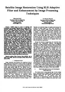
(4) where Vi and Vj denote two similarity patch-windows centered at the pixel i in the energy-specific image µbin and at the pixel j in the composite priori image µav that utilizes all available photons, respectively. Ni represents the search window in the image volume µav . In SCT imaging, the different photon counts in each energyspecific bin leads to the attenuation coefficient changes in the each resulting energy-specific image. Fig. 1 (a) shows a simulated x-ray beam spectra at 120 kV tube potentials [26]. The 120 kV spectrum was divided into 5 equally-distributed energy bins having equal width. Fig. 1 (b) shows that the difference in the attenuation coefficient ratio can be observed among the five regions of interest (ROIs) in Fig. 2 from Bin 2



(i.e., 40 keV to 60 keV) and Bin 5 (i.e., 100 keV to 120 keV). Therefore a local compensation factor C is naturally needed in Eq (3) to account for local intensity change. In this study, the compensation factor C is defined as follows: C (µbin (Vi ) , µav (Vj )) =

E (µbin (Vi )) E (µav (Vj ))

(5)

where E(·) denotes the expected value or mean of the intensity in the patch-window V .

2) Selection of the Smoothing Parameter: The smoothing parameter h in the NLM filter is usually designed as a function of the SD σ of the image noise (i.e., h = ασ) with a free scalar parameter α [25]. In addition, the average image µav has less noise level compared with the energy-specific image µbin . With the above-mentioned observation, h was empirically determined in this study with h2 = 2τ σ ¯ 2 |Ni | wherein σ ¯ denotes the SD of the average image µav . |Ni | denotes the size of the search window Ni , and τ is a scale factor.

5

x 10

2.5

Photon flux (counts)

Bin 1

Bin 2

Bin 3

Bin 4

Bin 5

5

4

3

2

1

atten. coeff. ratio difference

6

D. Image domain material decomposition

2

For the image-based basis material decomposition, the measurement in the CT image domain can be approximate as a linear combination of two basis materials [9], and the formulation of the material decomposition can be written as: µ ¶ µ ¶µ ¶ µH µ1H µ2H d1 = (7) µL µ1L µ2L d2

1.5 1 0.5 0

0

0

20

40

60

80

ROI A

100

ROI B

ROI C

ROI D

ROI E

Bin2 / Bin5

Photon energy (keV)

(a)

(b)

Fig. 1. (a) A simulated x-ray beam spectra at 120 kV tube potentials. The 120 kV spectrum was divided into 5 equally-distributed energy bins having equal width (20 keV); and (b) the attenuation coefficient ratio difference between Bin2 (i.e., 40-60 keV) and Bin5 (i.e., 100-120 keV) images of the five ROIs in Fig. 2.

3) Non-local Weighted Average: With the constructed nonlocal weights w(i, j), the proposed aviNLM algorithm for SCT image restoration can be performed through a non-local weighted average operation as follows: aviNLM(µbin (i)) =

X j∈Ni

w(i, j)µav (j).

(6)

From the weighted average of Eq. (6), the restored intensity values for the restored SCT images are from the average images. As a result, the noise-induced artifacts in the current SCT image are considerably suppressed in the restored SCT image because of the average image as a reference, which provides data redundancies for the restoration operation. C. Parameter Selections in the aviNLM Algorithm For SCT image restoration, three parameters in the aviNLM algorithm would be determined, i.e., the sizes of the search and patch-windows (i.e., Ni , Vi and Vj ) and the value of the smoothing parameter h. 1) Selection of the Search- and Patch- windows: In this study, we ran several preliminary experiments with different search-window Ni (i.e., 11×11, 15×15, 17×17 and 21×21) and performed quantitative measurements (i.e., the peak signal-to noise ratio, the contrast-to-noise ratio, and the universal quality index) and visual inspection compared with the ideal phantom or high-quality reference image. The related results showed that a 17×17 search-window Ni is adequate for effective noise and artifact suppression while retaining computational efficiency. In the implementation, the similarity of two patch windows with the size of 5×5 was measured by the conventional Euclidean distance wherein the selected patch in the µav contains additional information from the spectral component.

where µH/L denotes the reconstructed CT image at high or low energy spectrum, and the subscript H/L represents the high/low energy spectrum. d1/2 denotes the basis material image, and the subscripts 1 and 2 indicate two basis materials. µij is the linear attenuation coefficient of material i (i = 1 or 2) in mm−1 under energy spectrum j (j = H or L). The decomposition can be solved by directly performing signal decomposition via numerical matrix inversion or other superior techniques, such as least square method [7] and iterative decomposition method [27]. In this study, the decomposition is realized by numerical matrix inversion. E. Experimental Data Acquisition Numerical digital phantom, physical phantom and clinical patient data were used in the experiments to evaluate the performance of the present aviNLM algorithm for SCT image restoration. For the numerical simulation study, a modified clock phantom as shown in Fig. 2 that contains four different tissues (i.e., iodine, polyethylene, brain, and adipose) was used to generate the projection data with an energy-resolved detector. The modified clock phantom consists of a circular water background with the diameter of 28.0 cm and four large circular inserts, two medium circular inserts and one small circular insert with varying material (C1, C7: Iodine, 4.99 g/cm3 , C2, C6: Polyethylene, 0.97 g/cm3 , C3, C5: Brain, 1.039 g/cm3 , C4: Adipose, 0.95 g/cm3 ). For the physical phantom study, a cylindrical phantom (QSP-1, FUYO Corporation) with nine cylindrical tubes as shown in Fig. 3 was used to generate the SCT images with a commercial dualenergy CT. The diameter and length of the phantom is 20.0 cm and 13.0 cm, respectively. The outer and inner diameter of each tube is 2.5 cm and 1.80 cm with the length of 10.0 cm, respectively. The tubes #9 was filled with water located at the center of the phantom, whereas the other eight cylindrical tubes (#1 to #8) were filled with 50.0, 40.0, 30.0, 20.0, 15.0, 10.0, 5.0, 1.0 mg/mL of iodine contrast medium (Omnipaque, GE Healthcare) located symmetrically in the periphery of the phantom.



to Bin 5 for simplicity. The noisy sinogram for each energy bin was calculated with

Polyethylene

C2 ROI B

Brain

Ef (B)

1.

75

cm

Iodine

Φ

C5

C1 0

70

7.

Npoi (B) =

C7 C4

(11)

where B denotes a range of energy, and Es denotes the starting photon energy and Ef denotes the final energy. The resultant CT images can be yielded by a standard FBP approach with a Ramp filter [30]:

.0 28

Adipose

2.24 cm

(a)

Fig. 2.

Npoi (E),

ROI D

Φ

7.20 cm

X

E=Es (B)

cm

Φ

0.

Φ

C3 ROI C

ROI E

2.24 cm

cm

cm

ROI A

C6

(b)

µ µ ¶¶ D(B)S(B) µbin = FBP log . Npoi (B)

A modified clock phantom for numerical simulation study.

3 2

4

9

5

1 ROI C

ROI A

6

ROI B

8

7

ROI D

C1

(a)

C2

(b)

Fig. 3. A cylindrical phantom for real data study. (a) the phantom picture; and (b) one slice of CT images.

1) Numerical Simulation Study: The numerical simulation method is similar to the energy-resolved CT projection generation methods described in [7], [28]. For each attenuation map of the phantom at each energy (F (E)), Radon transform (R) was applied to obtain a noise-free sinogram data (G(E)): G(E) = R {F (E)} .

(8)

Then, the detected spectrum (N (E)) was first calculated from the noise-free sinogram data according to the BeerLambert law, N (E) = D(E)S(E)e−G(E) ,

(9)

where D(E) is the absorption efficiency of the detector, which is set to 1 in this study, and S(E) is the primary x-ray tube spectrum. Finally, Poisson noise to N (E) was injected into the detected spectrum to simulate the noisy transmission measurement Npoi (E), i.e., Npoi (E) = Poisson(N (E)),

(10)

where Poisson(λ) generates a random number from the Poisson distribution with a mean λ. In our study, an ideal energy-resolved detector was simulated with five different discriminator units to allow a binning of the detected pulses into user-selectable energy bins [29]. Fig. 1 (a) shows the five energy bins with [21, 40], [41, 60], [61, 80], [81,100], and [101,120] keV. The assumption here is that those photons with energy lower than 20 keV were totally absorbed by the intrinsic filters. The five energy bins are referred to as Bin 1

(12)

where D(B) denotes the mean absorption efficiency at specific energy bin and is set to 1 in our study, and S(B) denotes the number of incident X-ray intensity at each energy bin, and is set to be 2.8 × 105 , 3.2 × 105 , 3.5 × 105 , 2.1 × 105 and 2.0 × 105 , respectively. A geometry that was representative for a fan-beam CT scanner setup with a circular orbit to acquire 1160 views over 2π was chosen. The number of channels per view was 672 and the distance from the X-ray source to the detector was 104.0 cm. The distance from the rotation center to the curved detector was 47.0 cm. All the reconstructed images were represented with 512 × 512 array with 0.625 mm pixel size. 2) Physical Phantom Data Study: A 64-detector dualenergy CT scanner (Discovery CT750 HD GE) was used to scan the cylindrical phantom with four different tube potentials (i.e., 80, 100, 120, and 140 kVp) to acquire the SCT images. In all of the cases, the remaining CT parameters were set as follows: 0.6 s tube rotation time, 1.25 mm collimation, 600 mA tube current, 5 mm/5mm slice thickness and interval for the axial images, and 500 mm scan field of view (FOV). Gemstone Spectral Imaging viewer software (GE Healthcare) was used to process the projection data and review the images. The four sets of different energy projections registered in time and space were used to reconstruct CT images by using the manufacturer’s ‘standard’ reconstruction kernel. 3) Clinical Patient Data Study: The patient scan was scheduled for a head dual energy CT study for medical reasons. All head CT images were acquired with the 64detector dual-energy CT scanner (Discovery CT750 HD GE). In all of the cases, the scanning parameters were as follows: 0.6 s per gantry rotation, 1.25 mm collimation, 630 mA tube current, 5 mm/5mm slice thickness and interval for the axial images, and ‘standard reconstruction kernel’. Moreover, virtual monochromatic spectral (VMS) image with 60 keV was produced with the acquired dual energy CT images for comparison study. F. Evaluation Merits 1) Evaluation by Noise Reduction: The following metrics were used to measure the noise reduction on the restored images from the low-dose SCT images: (1) peak signal-tonoise ratio (PSNR); and (2) normalized mean square error



(NMSE), i.e., µ

max2 (µGS ) 2 k (µ(k) − µGS (k)) /(K − 1) P 2 (µ(k) − µGS (k)) NMSE = k P 2 k (µGS (k)) P

PSNR = 10 log10

¶ (13)

(14)

where µ(k) is the intensity value at pixel k in the image µ, µGS (k) is the intensity value at pixel k in the ideal phantom image, and K is the number of image pixels. max(µGS ) denotes the maximum intensity value of the ideal phantom image. 2) Evaluation by Contrast-to-noise Ratio Measure: Since a low-contrast region is of interest in the SCT imaging, we selected four ROIs (as indicated by squares with a size of 8x8 pixels in Fig. 2) to calculate the contrast-to-noise ratio (CNR), |¯ µROI − µ ¯BG | CNR = p 2 2 σROI + σBG

(15)

where µ ¯ROI is the mean of the pixels inside the ROI, and µ ¯BG is the mean of the pixels in the background. The terms σROI and σBG denote the SDs of the pixel values inside the ROI and in the background region, respectively. 3) Image-similarity Metric: The universal quality index (UQI) [31] was used in our study to measure the similarity between the reconstructed and truth samples. Given the aligned ROI within the reconstructed and ideal phantom images, the associated mean, variance and covariance over the ROI can be calculated as:

µ ¯=

M 1 X µ(m), M m=1

σ2 =

M X 1 (µ(m) − µ ¯)2 , (16) M − 1 m=1

M X 1 (µGS (m) − µ ¯GS )(µ(m) − µ ¯) M − 1 m=1 (17) where M denotes the number of pixels in the ROI. The UQI can be written as:

Cov {µ, µGS } =

U QI =

4Cov {µ, µGS } µ ¯·µ ¯GS · 2 2 σ 2 + σGS µ ¯ +µ ¯2GS

(18)

where µ and µGS denote the reconstructed and ideal phantom images. The value of UQI ranges between 0 and 1 and the value of UQI is closer to 1 when the reconstructed image is more similar to the original image. 4) Modulation Transfer Function: The resolution property of the present aviNLM algorithm was studied using a modulation transfer function (MTF), which characterizes the spatial resolution of images. For the MTF computation, an edge spread function (ESF) was first obtained along the profile at one axial direction on the insert as indicated by the red arrows in Fig. 2 (b) and Fig. 3 (b), respectively. The ESF was resampled using 1st order polynomial interpolation. The resampled ESF was averaged across multiple ESF realizations (measured at 3, 6, 9, and 12 o’clock positions) to yield the

ensemble ESF aiming to reduce noise in ESF. A line spread function (LSF) was then obtained from the derivation of the ensemble ESF. The resultant LSF was multiplied by a Hann window to remove the noise in tails [32]. By applying the Fourier transformation of the LSF, the MTF could be obtained. In this case, normalization may be needed so that MTF(0)=1. 5) Subjective Assessment: For subjective assessment, 5 radiologists with at least five years of experience in CT imaging scored the four virtual monochromatic spectral images by using different algorithms for each of the following attributes: image noise, artifacts, edge and structure, overall monochromatic image quality, and cylindrical tube size and boundary estimation with the same width, window level, and FOV. The scoring was done on a five-point scale: excellent is 5; good is 4; adequate is 3; suboptimal is 2; poor is 1. G. Other Experiments’ Settings To validate and evaluate the performance of the present aviNLM algorithm, the FBP algorithm with the Ramp filter, the HYPR-LR algorithm [3] and the NLM algorithm [25] were adopted for comparison. In the implementation of the HYPR-LR algorithm, we generated a composite image µav by averaging all of the images in the energy domain, and then performed an image filter operation on each individual energy image µbin and the composite image µav , and finally yielded a weighting image by the ratio between these two filtered images. Mathematically, the HYPR-LR algorithm is written as: HYPR(µbin ) =

µbin ⊗ T · µav µav ⊗ T

(19)

where T is a low-pass filter kernel. The symbol ⊗ denotes the convolution process. According to the analysis in [3], the noise variance of HYPR-LR images is mainly determined by the composite images, and streaks are reduced by normalizing the each individual energy image to the composite image. In this study, we ran several preliminary experiments with different filter sizes (i.e., 7 × 7, 9 × 9, and 11 × 11) and performed extensive experiments by quantitative measurements (i.e., PSNR, CNR, and UQI) and visual inspection compared to the ideal phantom and high-quality reference image, and we found that a Gaussian filter kernel with the size of 9 × 9 pixels was adequate to suppress noise and artifacts for all the cases in this study. In the implementation of the NLM algorithm, we modified its non-local weights by using the equation h2 = 2ασ 2 |Ni |, which considers the size of the search-window centered at pixel i. The SD σ of the energy-specific image µbin was estimated with a robust median estimator [33]. Extensive experiments showed that the search- and patch- windows with 17×17 and 5×5 sizes were also proper for the original NLM algorithm. The scale factors α for the NLM and τ for aviNLM algorithms was determined with trial-and-error method for visually appealing results compared with the ideal phantom or the high-quality reference image. All of the algorithms were implemented in Matlab R2011a (The MathWorks, Inc.) programming environment. The codes were run on a typical



desktop computer with Intel(R) Core (TM) i5-2400 Processor, 3.10 GHz, and 4 GB of RAM memory.

TABLE II CNR

MEASURE OF SECOND ENERGY BIN IMAGES FROM DIFFERENT ALGORITHMS .

Methods FBP HYPR-LR NLM aviNLM

III. R ESULTS A. Numerical Simulation Study Fig. 4 shows the images of the clock phantom reconstructed with four different algorithms. The upper row images show that the noise levels of the FBP image varied from one energy bin to another because the noise level of the FBP images not only depends on the different photon numbers available in each energy bin, but also depends on the energydependent linear attenuation coefficients of different materials. The images from the right energy ranges (e.g., 60 keV to 80 keV) had relatively lower noise levels than those from other energy ranges (e.g., 20 keV to 40 keV). The results from the second row to the fourth row demonstrate that the proposed aviNLM algorithm can yield remarkable gains over the other three algorithms in terms of noise-induced artifact suppression and resolution preservation at any energy range. Zoomed images of two ROIs, marked by the symbols C5 and C6 in Fig. 2, are drawn in Fig. 4 to further illustrate the gains of the aviNLM algorithm. Fig. 5 shows the MTFs obtained by the HYPR-LR, NLM and aviNLM algorithms in the first, second and third energy bin. We can observe that the aviNLM algorithm can yield a better image resolution than the other two algorithms in all the cases. Fig. 6 presents the results of the noise measures at the five ROIs (as indicated by squares with a size of 8x8 pixels in Fig. 2) from the five bin images yielded by four different algorithms. The figure depicts that the HYPR-LR, NLM, and aviNLM algorithms can achieve significant noise reduction; however, the aviNLM algorithm slightly outperforms the other two algorithms in that it achieved approximately 60% noise reduction in the five ROIs compared with the 30% and 50% noise reduction of the HYPR-LR and NLM algorithms, respectively. Fig. 7 shows the horizontal profiles through the center of both the brain insert (C5) and the polyethylene insert (C6) in the reconstructed images at five energy bins. The aviNLM algorithm yielded a profile closer to the truth compared with those of the other algorithms, especially in the edge region, as indicated by a black arrow in Fig. 7. The profile comparisons show that higher low-contrast detectability and more noticeable edge preservation can be achieved by the aviNLM algorithm than those of the other three algorithms. Tables I, II and III, show the CNR measures at the four ROIs (ROI A-ROI D) as indicated by squares in Fig. 2, wherein ROI E was used to measure the background noise level. It can be observed that the aviNLM filter can yield higher CNRs than the other three algorithms in all the cases. TABLE I CNR

MEASURE OF FIRST ENERGY BIN IMAGES FROM DIFFERENT ALGORITHMS .


ROI A 1.9687 2.0310 2.1953 2.3842

ROI B 1.3994 1.6272 1.8907 1.9056

ROI C 1.1574 1.9193 2.3273 2.4246

ROI D 1.2236 1.6538 1.7247 2.0653

ROI A 0.8201 1.2352 1.6377 2.4865

ROI B 0.9312 1.9575 2.0891 2.1324

ROI C 1.0578 1.8570 2.1214 2.1817

ROI D 1.6538 1.7547 2.0817 2.1654

TABLE III CNR

MEASURE OF THIRD ENERGY BIN IMAGES FROM DIFFERENT ALGORITHMS .


ROI A 1.1499 1.4191 1.5374 1.6458

ROI B 0.8449 1.0476 1.4809 1.5277

ROI C 1.2439 1.2568 1.6507 2.0330

ROI D 1.6014 1.7854 1.8475 1.9687

Tables IV and V show the NMSEs and PSNRs of the images reconstructed with the four different algorithms. The gains from the aviNLM algorithm are more noticeable compared with those from the other three algorithms in terms of NMSE and PSNR. In other words, the aviNLM algorithm can yield higher noise reduction than the other three algorithms in SCT image filtering. Fig. 8 shows the UQI values of the four regions indicated by the squares with the symbol Ci (i=1, 2, 3, 4) in Fig. 2. The gains from the aviNLM algorithm are more noticeable compared with those from the other three algorithms in terms of the UQI measure in the four regions. TABLE IV T HE NMSE S (×10−3 ) MEASURED IN EACH OF THE THREE ENERGY BINS FROM DIFFERENT ALGORITHMS . Methods Bin 1 Bin 2 Bin 3 Bin 4 Bin 5

FBP 1.25 1.26 1.10 1.21 1.16

HYPR-LR 1.18 1.22 1.09 1.10 1.17

NLM 1.06 1.07 0.978 0.957 0.987

aviNLM 0.667 0.686 0.970 0.945 0.969

TABLE V T HE PSNR S (dB) MEASURED IN EACH OF THE THREE ENERGY BINS FROM DIFFERENT ALGORITHMS . Methods Bin 1 Bin 2 Bin 3 Bin 4 Bin 5

FBP 39.686 40.001 39.614 38.768 38.887

HYPR-LR 39.957 40.133 39.624 39.184 38.861

NLM 40.432 40.691 40.138 39.793 39.597

aviNLM 42.425 42.629 40.170 39.849 39.677

Fig. 9 shows the decomposed images of basis materials from four different algorithms. In the implementation of decomposition, the iodine (material of the heighten area) and the water (material of the background) are chosen as the basis materials. The mean and standard deviations (SDs) in iodine are calculated on the ROI as indicated by a square in Fig. 9 (a) and the associated results are shown in Fig. 9 (e). It can be seen that the direct matrix inversion of the FBP images results in a high noise level of the decomposed image, but the noise level in the iodine images from the aviNLM algorithm is much



Bin 1

Bin 2

Bin 3

FBP

HYPR

NLM

aviNLM

Fig. 4. Images at the first [(21-40) keV]-third [(61-80) keV] (from left to right) energy bins obtained from simulation of a energy-resolved detector CT system. The 120 kVp spectrum was divided into five energy bins of equivalent width (20 keV). Images were reconstructed by a standard FBP technique, and restored by the HYPR-LR, NLM (αbin1 = 1.5 × 10−3 , αbin2 = 2.6 × 10−3 , αbin3 = 1.0 × 10−3 ) and aviNLM algorithms (τbin1 = 2.0 × 10−3 , τbin2 = 3.0 × 10−3 , τbin3 = 1.5 × 10−3 ). Two zoomed regions indicated by the marks with C5 and C6 are also shown. All the images are displayed with the same window: [0.005 0.035] mm−1 .

lower than that from the HYPR-LR and NLM algorithms. In other words, the aviNLM algorithm can outperform the other

three algorithms in differentiating iodine and water with a low noise level.


This article has been accepted for publication in a future issue of this journal, but has not been fully edited. Content may change prior to final publication. Citation information: DOI 10.1109/TBME.2015.2476371, IEEE Transactions on Biomedical Engineering 8 1

1

0.9

0.7

0.6

0.6

MTF

0.7

0.6 0.5

0.5

0.5

0.4

0.4

0.4

0.3

0.3

0.3

0.2

0.2

0.2

0.1

0.1

0.1

0

0 1

2

3

4

5

6

7

HYPR NLM aviNLM

0.8

0.7

0

0 0

1

2

Spatial Frequency (lp/cm)

3

4

5

6

7

0

1

2


(a)

3

4

5

6

7


(b)

(c)

MTF curves from the HYPR-LR, NLM and aviNLM algorithms in: (a) (21-40) keV; (b) (41-60) keV; and (c) (61-80) keV energy bins.

Noise (mm -1 )

-1

Noise (mm )

1.00E-03

8.00E-04

aviNLM

8.00E-04 6.00E-04 4.00E-04

1.40E-03

1.40E-03

FBP

Prior Image

HYPR

NLM

aviNLM

6.00E-04

4.00E-04

FBP

Prior Image

HYPR

NLM

1.20E-03

1.40E-03 FBP

Prior Image

HYPR

NLM

aviNLM

8.00E-04 6.00E-04 4.00E-04

FBP

Prior Image

HYPR

NLM

1.20E-03

1.20E-03

1.00E-03

-1

Prior Image NLM

Noise (mm -1 )

1.00E-03 FBP HYPR

1.20E-03

Noise (mm -1 )

1.40E-03

Noise (mm )

Fig. 5.

0.9

HYPR NLM aviNLM

0.8

MTF

MTF

0.8

1

0.9

HYPR NLM aviNLM

1.00E-03 aviNLM

8.00E-04 6.00E-04 4.00E-04

1.00E-03 aviNLM

8.00E-04 6.00E-04 4.00E-04

2.00E-04 2.00E-04

2.00E-04 0.00E+00

0.00E+00

Bin 1

Bin 2

Bin 3

Bin 4

0.00E+00

0.00E+00

Bin 1

Bin 5

Bin 2

(a)

Bin 3

Bin 4

2.00E-04

2.00E-04

Bin 5

Bin 1

Bin 2

Bin 3

(b)

Bin 4

0.00E+00

Bin 5

Bin 1

Bin 2

Bin 3

(c)

Bin 4

Bin 1

Bin 5

Bin 2

(d)

Bin 3

Bin 4

Bin 5

(e)

Fig. 6. Image noise measured at the five ROIs in each of the five energy bins. (a) noise measure of ROI A; (b) noise measure of ROI B; (c) noise measure of ROI C; (d) noise measure of ROI D; and (e) noise measure of ROI E. 0.028

0.028 0.026 Phantom HYPR NLM aviNLM

0.024 0.022

0.024 0.022 0.02 Phantom HYPR NLM aviNLM

0.018 0.016

0.02 220

240

260

280

300

320


0.014

0.014 200

0.02

0.017

220

240

260

280

300

320

0.017 0.016 0.015 Phantom HYPR NLM aviNLM

0.014

220

240

260

280

300

220

Pixel Position

(b)


0.013

0.011 200

320

0.016

0.012

0.012 200

Pixel Position

(a)

0.018

0.013

0.012 200

Pixel Position

0.019

Image Intensity

0.03

0.018

0.02 0.022

Image Intensity

0.032

0.021

0.024

0.026

0.034

Image Intensity

Image Intensity

0.036

Image Intensity

0.038

240

260

280

300

320

200

Pixel Position

(c)

220

240

260

280

300

320

Pixel Position

(d)

(e)

1.00 0.90 0.80 0.70 0.60 0.50 0.40 0.30 0.20 0.10 0.00

UQI

1.00 0.90 0.80 0.70 0.60 0.50 0.40 0.30 0.20 0.10 0.00

UQI

1.00 0.90 0.80 0.70 0.60 0.50 0.40 0.30 0.20 0.10 0.00

UQI

0.92 0.90 0.88 0.86 0.84 0.82 0.80 0.78 0.76 0.74 0.72

UQI

UQI

Fig. 7. Horizontal profiles through the center of both the brain insert (C5) and the polyethylene insert (C6) in the reconstructed clock phantom images corresponding to five energy bins. (a) the profile of the first energy bin; (b) the profile of the second energy bin; (c) the profile of the third energy bin; (d) the profile of the fourth energy bin; and (e) the profile of the fifth energy bin. The profiles located at the pixel position x from 192 to 315 and y=256. The ‘black solid line’ denotes the profiles of the ground-truth; the ‘green solid line’ donates the profiles of the HYPR-LR algorithm; the ‘dot-dashed line’ denotes the profiles from the NLM algorithm; and the ‘dashed line’ denotes the profiles from the aviNLM algorithm. The unit is mm−1 . 1.00 0.90 0.80 0.70 0.60 0.50 0.40 0.30 0.20 0.10 0.00

ROI A

ROI B

ROI C

ROI D

ROI A

ROI B

ROI C

ROI D

ROI A

ROI B

ROI C

ROI D

ROI A

ROI B

ROI C

ROI D

FBP

0.7924

0.8266

0.8251

0.7949

FBP

0.7421

0.8218

0.7070

0.7867

FBP

0.8148

0.8474

0.7235

0.8133

FBP

0.8860

0.8629

0.7321

0.8248

FBP

0.8931

0.8709

0.7531

0.8350

NLM

0.8634

0.8533

0.8513

0.8117

NLM

0.8132

0.8393

0.8407

0.8223

HYPR

0.8166

0.8560

0.7634

0.8293

HYPR

0.8883

0.8687

0.7599

0.8369

HYPR

0.8937

0.8724

0.7600

0.8382

HYPR

0.8687

0.8897

0.8741

0.8655

HYPR

0.8444

0.8581

0.8804

0.8678

NLM

0.8185

0.8753

0.8547

0.8721

NLM

0.8917

0.8913

0.8660

0.8865

NLM

0.8968

0.8925

0.8459

0.8789

aviNLM

0.8855

0.8917

0.9099

0.8947

aviNLM

0.8512

0.8874

0.9013

0.8881

aviNLM

0.8374

0.8965

0.8985

0.8881

aviNLM

0.9101

0.9114

0.8916

0.9007

aviNLM

0.9062

0.9126

0.9051

0.8979

(a)

(b)

(c)

ROI A

ROI B

ROI C

ROI D

(d)

(e)

Fig. 8. UQIs of four regions indicated by the squares with the symbol Ci (i=1,2,3,4) in Fig. 2 from the reconstructed images by four different algorithms from five energy bin. (a) UQI measure of first energy bin images; (b) UQI measure of second energy bin images; (c) UQI measure of third energy bin images; (d) UQI measure of fourth energy bin images; and (e) UQI measure of fifth energy bin images.

B. Physical Phantom Data Study Fig. 10 shows the images of the real phantom from four different algorithms. From the upper row to the bottom row, it can be seen that the images reconstructed by the HYPRLR, NLM and aviNLM algorithms were better than that from the FBP algorithm in terms of visual inspection. Noticeable differences among the results can be observed at the two selected ROIs marked by the symbols C1 and C2 in Fig. 3 (b). As a result, the aviNLM algorithm achieves significant gains

over the other algorithms in terms of both noise suppression and edge preservation. In addition, we calculated the mean and SD of the CT number of three red square ROIs (i.e., squares A, B and C) in Fig. 3 (b) to quantitatively evaluate image quality, and the associated results are shown in Fig. 11. The aviNLM algorithm can reach higher restoration accuracy than HYPR-LR and NLM algorithms, as measured by the SD of the image density within each ROI. Fig. 12 shows the MTFs of the restored physical phantom



ROI

(a)

(b)

Iodine Intensity (g/cm3)

5.3

5.2

5.1

5

4.9

4.8

4.7

FBP

HYPR

NLM

aviNLM

Method

(e) (c)

(d)

Fig. 9. Decomposed images of basis materials and comparison of basis material concentration obtained using different algorithms. Left column: the iodine images from the material decomposition method after the FBP algorithm (a), HYPR-LR algorithm (b), NLM algorithm (c) and aviNLM algorithm (d) processing. All iodine images are displayed at the same window: [0 5.4] g/cm3 . Right column: decomposed iodine concentration as a function of different algorithm. The iodine concentration during simulations was 4.99 g/cm3 . The error bars represent the standard deviation.

images by the HYPR-LR, NLM and aviNLM algorithms, respectively. It can be observed that the spatial resolution of the restored images by the aviNLM algorithm is much better than that from the other two algorithms. Fig. 13 shows the decomposed basis material images from four different algorithms wherein the iodine and water were chosen as the basis materials and the mass attenuation coefficients of these two basis materials are accessible with instruction from the CT vendor. It can be observed that the noise level in both water and iodine images from the aviNLM algorithm is lower than the other three algorithms. Furthermore, to illustrate the precision of the material decompositions, the concentrations of water and iodine at ROI C in #1 and ROI D in #8 as indicated in Fig. 3 are estimated and depicted with the histograms, respectively. The results are shown in Fig. 14, which illustrate the accuracy and precision of the material decompositions within the included material tubes #1 and #8. The expected concentrations of water and iodine in #1 and #8 are (1000 mg/mL, 1.0 mg/mL) and (1000 mg/mL, 50 mg/mL), respectively. In addition, the expected concentration are also included and indicated by vertical lines for comparison. It can be seen that the correlations between the expected and measured material concentrations of iodine and water within both tubes from the aviNLM algorithm are stronger than that from the other three algorithms.

The LSNR is defined as the ratio of the mean and standard deviation of the intensity in each local region. It can be seen that the LSNR of the restored images by the aviNLM algorithm is higher than that from the other two restoration algorithms. Furthermore, Fig. 16 shows the VMS images (60 keV) generated from these images. The aviNLM algorithm can yield the noticeable gains over the other three algorithms in term of noise suppression of VMS images. In addition, Table VIII lists the subjective scores in the four images, which indicates that the aviNLM algorithm can yield higher subjective image score than the other three algorithms in generating high-quality VMS images. TABLE VI LSNR

MEASUREMENTS OF 80 K V P IMAGES FROM DIFFERENT ALGORITHMS .

Methods LSNR (ROI 1) LSNR (ROI 2)

FBP 20.369 11.145

HYPR-LR 50.558 32.605

NLM 80.269 33.591

aviNLM 100.125 33.845

TABLE VII LSNR

MEASUREMENTS OF 140 K V P IMAGES FROM DIFFERENT ALGORITHMS .

Methods LSNR (ROI 1) LSNR (ROI 2)

FBP 11.371 17.445

HYPR-LR 22.041 32.105

NLM 23.345 33.592

aviNLM 34.163 43.145

C. Clinical Patient Data Study Fig. 15 shows the real patient CT images restored by four different algorithms. It can be seen that the results from the HYPR-LR, NLM and aviNLM algorithms have noticeable gains over that from the FBP algorithm in terms of visual inspection. Tables VI and VII list the local signal-to-noise ratio (LSNR) of two blue square ROIs as indicated in Fig. 15.

TABLE VIII S UBJECTIVE SCORES OF VMS IMAGES (60 ALGORITHMS . Methods Subjective scores

FBP 2.32±0.55

HYPR-LR 3.52±0.77

KE V) FROM DIFFERENT

NLM 3.90±0.85


aviNLM 4.15±0.58


80 kVp

100 kVp

120 kVp

140 kVp

FBP

HYPR

NLM

aviNLM

Fig. 10. Images reconstructed using the standard FBP, HYPR-LR, NLM (α80 = 1.0×10−3 , α100 = 1.5×10−3 , α120 = 1.2×10−3 , α140 = 1.9×10−3 ) and aviNLM algorithms (τ80 = 8.0 × 10−2 , τ100 = 4.0 × 10−2 , τ120 = 1.5 × 10−2 , τ140 = 3.0 × 10−2 ) from a clinical dual energy CT scanner using an integrating detector system with tube potentials of 80, 100, 120, and 140 kVp from left to right. The ROIs indicated by the dashed squares in Fig. 3 are zoomed in to display the image details. All the images are displayed with the same window: [500 2000] HU. 1000

Original

1750

HYPR

NLM

3200

aviNLM

Original

HYPR

NLM

aviNLM

Original

HYPR

NLM

aviNLM

980 3000

1650 1600 1550 1500 1450 1400

960

Image Intensity

Image Intensity

Image Intensity

1700

940 920 900 880 860 840

1350

80

100

120

140

2800

2600

2400

2200

2000

80

100

120

140

80

100

120

140

820

kV

kV

kV

(a)

(b)

(c)

Fig. 11. Mean image density and image noise measured at the three ROIs (i.e., squares A, B and C) in each of the four tube potentials in Fig. 10 using the standard FBP, HYPR-LR, NLM and aviNLM algorithms. The error bars represent one standard deviation. The unit is HU.


This article has been accepted for publication in a future issue of this journal, but has not been fully edited. Content may change prior to final publication. Citation information: DOI 10.1109/TBME.2015.2476371, IEEE Transactions on Biomedical Engineering 11 1

1

HYPR NLM aviNLM

0.9

0.8

0.7

0.7

0.6

0.6

MTF

MTF

0.8

0.5

HYPR NLM aviNLM

0.9

0.5

0.4

0.4

0.3

0.3

0.2

0.2

0.1

0.1

0

0 0

0.5

1

1.5

2

2.5

3

3.5

4

0

0.5

1


1.5

(a)

2.5

3

3.5

4

(b)

1

1

HYPR NLM aviNLM

0.9 0.8

0.8

0.7

0.7

0.6

0.6

0.5

0.5

0.4

0.4

0.3

0.3

0.2

0.2

0.1

0.1

0

HYPR NLM aviNLM

0.9

MTF

MTF

2


0 0

0.5

1

1.5

2

2.5

3

3.5

4

0

0.5

1


1.5

2

2.5

3

3.5

4


(c)

(d)

Fig. 12. MTF curves from the HYPR-LR, NLM and aviNLM algorithms in four different cases. (a) is the case of 80 kVp; (b) is the case of 100 kVp; (c) is the case of 120 kVp; and (d) is the case of 140 kVp.

FBP

HYPR

NLM

aviNLM

Water

Iodine

Fig. 13. Decomposed images of basis materials. Row one: the water images from the material decomposition algorithm after the FBP, HYPR-LR, NLM and aviNLM processing. Row two: the Iodine images from material decomposition method after the FBP, HYPR-LR, NLM and aviNLM processing, respectively. All water image are displayed at the same window: [0 1000] mg/mL and all iodine image are displayed at the same window: [-5 30] mg/mL.

IV. D ISCUSSION The original NLM algorithm restores the intensity of each image pixel by averaging the intensities of its neighboring pixels. The averaging weight is based on self-similarity in images through comparison of local neighborhoods. The similarity between a given pixel pair is robustly derived from the intensity differences between the patches of neighboring pixels

surrounding them. Conceptually, the averaging weights can be interpreted as a probability distribution with normalization to unity and is always positive. Clearly, optimizing the weights plays a crucial role in the NLM algorithm. Up to now, many NLM-based methods have been proposed to yield optimal nonlocal weights [24], [34], [35]. In this study, an alternative strategy called aviNLM algorithm is proposed to design the


This article has been accepted for publication in a future issue of this journal, but has not been fully edited. Content may change prior to final publication. Citation information: DOI 10.1109/TBME.2015.2476371, IEEE Transactions on Biomedical Engineering 12 0.25

0.7

Phantom HYPR NLM aviNLM

known concentration of iodine in #1 0.2

0.6


known concentration of iodine in #8

Fraction

Fraction

0.5 0.15

0.1

0.4

0.3

0.2 0.05 0.1

0 35

40

45

50

55

0 -8

60

-6

-4

Concentration (mg/mL)

-2

0

2

4

6

8


(a)

(b)

0.015

0.02


known concentration of water in #1

0.018

known concentration of water in #8


0.016 0.014

Fraction

Fraction

0.01 0.012 0.01 0.008

0.005 0.006 0.004 0.002

0 700

800

900

1000

1100

1200

1300


0 800

850

900

950

1000

1050

1100

1150

1200


(c)

(d)

Fig. 14. Histograms of material concentrations measured in the #1 and #8 tubes through the HYPR-LR, NLM, and aviNLM algorithms. (a) Histograms of material concentrations of iodine in the #1 wherein a purple vertical line in the histogram indicates the known concentration of iodine in #1; (b) Histograms of material concentrations of iodine in the #8 wherein a cyan vertical line in the histogram indicates the known concentration of iodine in #8; (c) Histograms of material concentrations of water in the #1 wherein a purple vertical line in the histogram indicates the known concentration of water in #1; and (d) Histograms of material concentrations of water in the #8 wherein a cyan vertical line in the histogram indicates the known concentration of water in #8.

FBP

80 kVp

HYPR

NLM

aviNLM

ROI 1 ROI 2

140 kVp

ROI 1 ROI 2

Fig. 15. Images from the standard FBP, HYPR-LR, NLM (α80 = 3.0 × 10−3 , α140 = 5.0 × 10−3 ) and aviNLM algorithms (τ80 = 8.0 × 10−2 , τ140 = 4.0 × 10−2 ) where the original data were acquired by using a dual energy CT scanner with tube potentials of 80 and 140 kVp from top to bottom. All the images are displayed with the same window: [900 1250] HU.

weights for SCT image restoration on the basis of our previous work [24], [36], [37], [38]. The experimental results in Section III have shown that the aviNLM algorithm can yield more significant performance gains than the existing HYPR-LR and

NLM algorithms in terms of different measurement metrics. The redundant information in the whole energy domain was exploited to optimize the construction of weights and improve the NLM weighted average. The gain from using the redundant



FBP

HYPR

NLM

aviNLM

(a)

(b)

(c)

(d)

Fig. 16. Virtual monochromatic spectral (VMS) images (60 keV) generated from 80 and 140 kVp images. (a) is from the FBP algorithm; (b) is from the HYPR-LR algorithm; (c) is from the NLM algorithm; and (d) is from the aviNLM algorithm. All the images are displayed with the same window: [900 1250] HU.

information over the spectral domain is noticeable. In this study, the weights of the aviNLM algorithm were calculated by incorporation of an average image generated from the images reconstructed at all energy bins. In the implementation, other image generation methods can also be adapted into the aviNLM algorithm in the image domain, such as the maximum intensity projection volume (MIP) of the SCT images in all energy domains and optimally weighted SCT images [39]. For the present aviNLM algorithm, an average image generated from the images reconstructed in all energy bins provides strong a priori information on the patient and is a logical choice to induce SCT image restoration. In most SCT systems, such as photon-counting CT and dual-energy CT systems, the image data at different energy bins are simultaneously obtained; therefore, tissue deformation is of minimal concern. For slow-kVp based SCT systems, misalignments across the individual energy bins may be observed in the patient’s anatomy because of tissue deformation. Therefore, for the HYPR-LR algorithm dedicated image registration techniques are needed to fully use the prior-image of the same patient because it is a pixel-based image filtering operation with the assumption of prior- and objective image being aligned pixel by pixel. Meanwhile, as previously discussed [24], the challenge of tissue deformation may not be a major obstacle for the ndiNLM algorithm because the algorithm does not heavily depend on the accuracy of the image registration. Consequently, an important novelty of the present aviNLM algorithm in this study is the utilization of the images in all energy bins without the need for accurate image registration. In this approach, some parameters need to be determined. Optimizing parameters is a critical problem, and determining the best parameters is an empirical, subjective, and timeconsuming trial-and-error process. Additionally, analyzing the relationship between noise and structure information in the noise reduction process is possible. As described in Section II-C, a comparison of the quantitative measures and visual inspection on the ideal phantom or high-quality reference image helped to empirically determine the parameters for the aviNLM algorithm in a trial-and-error manner. In practical applications, determining all of the parameters should be adaptive, but this task is difficult. Therefore, additional theoretical

insights into optimizing the parameters are necessary, and these may be a topic for future research. V. C ONCLUSION In this study, we proposed an average image-induced nonlocal means (aviNLM) filter for SCT image restoration based on our previous studies [24], [36], [37], [38]. Specifically, the proposed aviNLM filter yields the restored results by performing a non-local weighted average operation on the noisy energy-specific images with the non-local weight matrix between the target and prior images, in which the prior image is generated from all of the images reconstructed in each energy bin. The experimental results in Section III have shown that the aviNLM algorithm can yield more significant performance gains than the existing HYPR-LR and NLM algorithms in terms of different measurement metrics. In other words, the proposed aviNLM algorithm has useful potential for radiation dose reduction by lowering the mAs in SCT imaging. ACKNOWLEDGMENT The authors would like to thank the anonymous reviewers for their constructive comments and suggestions that greatly improve the quality of the manuscript. R EFERENCES [1] P. M. Shikhaliev et al., “Photon counting computed tomography: Concept and initial results,” Med. Phys., vol. 32, p. 427, Jan. 2005. [2] P. M. Shikhaliev, “Photon counting spectral CT: Improved material decomposition with K-edge-filtered x-rays,” Phys. Med. Biol., vol. 57, pp. 1595-615, Mar. 2012. [3] S. Leng et al., “Noise reduction in spectral CT: Reducing dose and breaking the trade-off between image noise and energy bin selection,” Med. Phys., vol. 38, p. 4946, Aug. 2011. [4] R. E. Alvarez and A. Macovski, “Energy-selective reconstructions in Xray computerized tomography,” Phys. Med. Biol., vol. 21, pp. 733-44, Sep. 1976. [5] W. A. Kalender et al., “Evaluation of a prototype dual-energy computed tomographic apparatus. I. Phantom studies,” Med. Phys., vol. 13, pp. 334-9, Jan. 1986. [6] D. J. Walter et al., “Accuracy and precision of dual energy CT imaging for the quantification of tissue fat content,” in Proc. SPIE Med. Imag., 2006, vol. 6142, pp. 61421G. [7] H. Q. Le and S. Molloi, “Least squares parameter estimation methods for material decomposition with energy discriminating detectors,” Med. Phys., vol. 38, p. 245, Dec. 2010.



[8] M. Barreto et al., “Potential of dual-energy computed tomography to characterize atherosclerotic plaque: ex vivo assessment of human coronary arteries in comparison to histology,” Journal of Cardiovascular Computed Tomography, vol. 2, pp. 234-42, Aug. 2008. [9] B. Heismann et al., Spectral computed tomography. Belingham, Washington USA: SPIE, 2012, pp. 25-87. [10] K. Taguchi and J. S. Iwanczyk, “Vision 20/20: Single photon counting x-ray detectors in medical imaging,” Med. Phys., vol. 40, p. 100901, Sep. 2013. [11] P. M. Shikhaliev, “Tilted angle CZT detector for photon counting/energy weighting x-ray and CT imaging,” Phys. Med. Biol., vol. 51, pp. 426787, Aug. 2006. [12] Y. Alivov et al., “Optimization of K-edge imaging for vulnerable plaques using gold nanoparticles and energy resolved photon counting detectors: A simulation study,” Phys. Med. Biol., vol. 59, p. 135, Jan. 2014. [13] P. Sukovic and N. H. Clinthorne, “Penalized weighted least-squares image reconstruction for dual energy X-ray transmission tomography,” IEEE Trans. Med. Imaging, vol. 19, pp. 1075-81, Nov. 2000. [14] J. A. Fessler et al., “Maximum-likelihood dual-energy tomographic image reconstruction,” in Proc. SPIE Med. Imag., 2002, vol. 4684, pp. 38-49. [15] J. A. O’Sullivan and J. Benac, “Alternating minimization algorithms for transmission tomography,” IEEE Trans. Med. Imaging, vol. 26, pp. 283-97, Mar. 2007. [16] W. Huh and J. A. Fessler, “Model-based image reconstruction for dualenergy X-ray CT with fast KVP switching,” in Proc IEEE international symposium on biomedical imaging: from nano to macro (ISBI), 2009, pp. 326-9. [17] R. Zhang et al., “Model-based iterative reconstruction for dual-energy X-ray CT using a joint quadratic likelihood model,” IEEE Trans. Med. Imaging, vol. 33, pp. 117-34, Jan. 2014. [18] J. Noh et al., “Low-dose dual-energy computed tomography for PET attenuation correction with statistical sinogram restoration,” in Proc. SPIE Med. Imag., 2008, vol. 6913, p. 691312. [19] J. Noh et al., “Statistical sinogram restoration in dual-energy CT for PET attenuation correction,” IEEE Trans. Med. Imaging, vol. 28, pp. 1688-702, Nov. 2009. [20] W. Huh and J. A. Fessler, “Iterative image reconstruction for dual-energy X-ray CT using regularized material sinogram estimates,” in Proc IEEE international symposium on biomedical imaging: from nano to macro (ISBI), 2011, pp. 1512-5. [21] R. A. Rutherford et al., “Measurement of effective atomic number and electron density using an EMI scanner,” Neuroradiology, vol. 11, pp. 15-21, May. 1976. [22] W. A. Kalender et al., “An algorithm for noise suppression in dual energy CT material density images,” IEEE Trans. Med. Imaging, vol. 7, pp. 218-24, Sep. 1988. [23] R. A. Rutherford et al., “X-ray energies for effective atomic number determination,” Neuroradiology, vol. 11, pp. 23-8, May 1976. [24] J. Ma et al., “Low-dose computed tomography image restoration using previous normal-dose scan,” Med. Phys., vol. 38, p. 5713, Sep. 2011. [25] A. Buades et al., “A review of image denoising algorithms, with a new one,” Multiscale Modeling & Simulation, vol. 4, pp. 490-530, Jul. 2005. [26] J. M. Boone and J. A. Seibert, “An accurate method for computergenerating tungsten anode x-ray spectra from 30 to 140 kV,” Med. Phys., vol.24, pp. 1661-70, Aug. 1997. [27] X. Dong et al., “Combined iterative reconstruction and image-domain decomposition for dual energy CT using total-variation regularization,” Med. Phys., vol.41, p. 051909, Aug. 2014. [28] P. M. Shikhaliev, “Beam hardening artefacts in computed tomography with photon counting, charge integrating and energy weighting detectors: a simulation study,” Phys. Med. Biol., vol. 50, pp. 5813-27, Nov. 2005. [29] J. P. Schlomka et al., “Experimental feasibility of multi-energy photoncounting K-edge imaging in pre-clinical computed tomography,” Phys. Med. Biol., vol. 53, pp. 4031-47, Jul. 2008. [30] A. C. Kak and M. Slaney, Principles of computerized tomographic imaging. New York: IEEE, 1988, pp. 203-270. [31] Z. Wang and A. Bovik, “A universal image quality index,” IEEE Signal Processing Letters, vol. 9, pp. 81-4, Mar. 2002. [32] S. Richard et al., ”Towards task-based assessment of CT performance: System and object MTF across different reconstruction algorithms,” Med. Phys., vol. 39, pp. 4115-22, June 2012. [33] D. L. Donoho and J. Johnstone, “Ideal spatial adaptation by wavelet shrinkage,” Biometrika, vol. 81, pp. 425-55, Sep. 1994. [34] P. Coupe et al., “An optimized blockwise nonlocal means denoising filter for 3-D magnetic resonance images,” IEEE Trans. Med. Imaging, vol. 27, pp. 425-41, Apr. 2008.

[35] Y. Gal et al., “Denoising of dynamic contrast-enhanced MR images using dynamic nonlocal means,” IEEE Trans. Med. Imaging, vol. 29, pp. 302-10, Feb. 2010. [36] Z. Bian et al., “SR-NLM: A sinogram restoration induced non-local means image filtering for low-dose computed tomography,” Comput. Med. Imaging and Graph., vol. 37, pp. 293-303, Jun. 2013. [37] J. Huang et al., “Projection data restoration guided non-local means for low-dose computed tomography reconstruction,” in Proc IEEE international symposium on biomedical imaging: from nano to macro (ISBI), 2011, pp. 1167-70. [38] J. Ma et al., “Iterative image reconstruction for cerebral perfusion CT using a pre-contrast scan induced edge-preserving prior,” Phys. Med. Biol., vol. 57, pp. 7519-42, Oct. 2012. [39] T. G. Schmidt, “Optimal “image-based” weighting for energy-resolved CT,” Med. Phys., vol. 36, p. 3018, Jun. 2009.
