Speech Recognition on an FPGA Using Discrete and ... - CiteSeerX

Speech Recognition on an FPGA Using Discrete and Continuous Hidden Markov Models Stephen J. Melnikoff, Steven F. Quigley & Martin J. Russell Electronic, Electrical and Computer Engineering, University of Birmingham, Edgbaston, Birmingham, B15 2TT, United Kingdom [email protected]

Presented at: 12th International Conference on Field Programmable Logic and Applications (FPL 2002) Published in: Lecture Notes in Computer Science #2438, pp.202-211

© Springer-Verlag

The original publication is available at www.springerlink.com http://www.springerlink.com/content/12lmfc9httabcrae

Speech Recognition on an FPGA Using Discrete and Continuous Hidden Markov Models Stephen J. Melnikoff, Steven F. Quigley & Martin J. Russell Electronic, Electrical and Computer Engineering, University of Birmingham, Edgbaston, Birmingham, B15 2TT, United Kingdom [email protected], [email protected], [email protected]

Abstract. Speech recognition is a computationally demanding task, particularly the stage which uses Viterbi decoding for converting pre-processed speech data into words or sub-word units. Any device that can reduce the load on, for example, a PC’s processor, is advantageous. Hence we present FPGA implementations of the decoder based alternately on discrete and continuous hidden Markov models (HMMs) representing monophones, and demonstrate that the discrete version can process speech nearly 5,000 times real time, using just 12% of the slices of a Xilinx Virtex XCV1000, but with a lower recognition rate than the continuous implementation, which is 75 times faster than real time, and occupies 45% of the same device.

1 Introduction Real time continuous speech recognition is a computationally demanding task, and one which tends to benefit from increasing the available computing resources. A typical speech recognition system starts with a pre-processing stage, which takes a speech waveform as its input, and extracts from it feature vectors or observations which represent the information required to perform recognition. The second stage is recognition, or decoding, which is performed using a set of phoneme-level statistical models called hidden Markov models (HMMs). In most systems, several contextsensitive phone-level HMMs are used, in order to accommodate context-induced variation in the acoustic realisation of the phone. Word-level acoustic models are formed by concatenating phone-level models according to a pronunciation dictionary. The word models are then combined with a language model, which constrains the recogniser to recognise only valid word sequences. For small- to medium-sized vocabularies the word and language models are compiled into a single, integrated model. Recognition is performed using the Viterbi algorithm to find the route through this model which best explains the data. For large vocabulary systems this approach is not viable, and some form of heuristic search strategy, such as stack-decoding, is used instead [11]. The pre- and post-processing stages can be performed efficiently enough in software. The decoder, however, places a particularly high load on the processor, and

so it is this part of the system that has been the subject of implementations in hardware. Research has been carried out in the past on such implementations, generally using custom hardware, as described in section 4. However, with ever more powerful programmable logic devices being available, such chips appear to offer an attractive alternative. Accordingly, in this paper we describe our implementation of an HMM-based speech recognition system, with separate discrete and continuous HMM versions, which makes use of an FPGA for the decoder stage. This work follows on from that introduced in [4,5]. The paper is organised as follows. Section 2 explains the motivation behind the research; this is followed in section 3 by an overview of speech recognition theory. In section 4, we look at other hardware speech recognition systems, including implementations on FPGAs, custom hardware, ASICs and cores. We describe the structure of our system in section 5, followed by details of the implementations and discussion of the results in section 6. Section 7 summarises the conclusions drawn so far, and describes ideas to be incorporated into future implementations.

2 Motivation The ultimate aim of this work is to produce a hardware implementation of a speech recognition system, with an FPGA acting as a co-processor that is capable of performing recognition at a much higher rate than software. For most speech recognition applications, it is sufficient to produce results in real time, and software solutions that perform recognition in real time already exist. However, there are several scenarios that require much higher recognition rates which can benefit from hardware acceleration. For example, there are telephony-based applications used for call centres (e.g. the AT&T “How may I help you?” system [2]), where the speech recogniser is required to process a large number of spoken queries in parallel. There are also analogous nonreal time applications, such as off-line transcription of dictation, where the ability of a single system to process multiple speech streams at high speed may offer a significant financial advantage. Alternatively, the additional processing power offered by an FPGA might be used for real-time implementation of the “next generation” of speech recognition algorithms, which are currently being developed in laboratories. For example, improved recognition of fluent, conversational speech may require multiple-level acoustic models which incorporate a representation of the speech production process, and are able to accommodate the production strategies which individuals employ in fluent speech. Such models are much more complex than conventional HMMs and, if successful, will inevitably lead to a substantial increase in demand for computing power for speech recognition applications.

b0(Ot) a00

0

b1(Ot) a11

a01

1

b2(Ot) a22

a12

2

a02

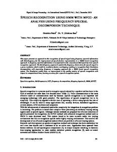
Fig. 1. Finite state machine for a Hidden Markov Model, showing the paths between states within the HMM (filled arrows), and paths between HMMs (unfilled arrows). The probability of a transition from state i to state j (transition probability aij) is shown, as is the probability of each state emitting the observation corresponding to time t (observation probability bj(Ot) for each state j) (double-headed arrows)

3 Speech Recognition Theory The most widespread and successful approach to speech recognition is based on the Hidden Markov Model (HMM), which is a probabilistic process that models spoken utterances as the outputs of finite state machines. A very brief outline is given below. For a more detailed description of HMM theory, see [7], or for an overview of the theory as it relates to this implementation, see our previous paper [5]. The notation here is based on [7]. 3.1 Hidden Markov Models The

underlying

problem

is

as

follows.

Given

an

observation

sequence

O = O0 , O1... OT −1 , where each Ot is data representing speech which has been sampled

at fixed intervals, and a number of potential models, each of which is a representation of a particular spoken utterance (e.g. word or sub-word unit), we would like to find the sequence of models which is the most likely to have produced O. These models are based on HMMs. An N-state Markov Model is completely defined by a set of N states forming a finite state machine, and an N × N stochastic matrix defining transitions between states, whose elements aij = P(state j at time t | state i at time t−1) are the transition probabilities. With a Hidden Markov Model (Fig. 1), each state additionally has associated with it a probability density function bj(Ot) which determines the probability that state j emits a particular observation Ot at time t (the model is “hidden” because any state could have emitted the current observation). The p.d.f. can be continuous or discrete; accordingly the pre-processed speech data can be a multi-dimensional vector or a single quantised value. bj(Ot) is known as the observation probability. Such a model can only generate an observation sequence O = O0 , O1 ... OT −1 via a state sequence of length T, as a state only emits one observation at each time t. Our aim is to find the state sequence which has the highest probability of producing the observation sequence O. This can be approximated efficiently using Viterbi decoding.

3.2 Viterbi Decoding We define the value δt(j), which is the maximum probability that the HMM is in state j at time t. It is equal to the probability of the most likely partial state sequence which emits observation sequence O = O0 , O1 ... Ot , and which ends in state j. It can be shown that this value can be computed iteratively as: δt ( j ) = max [δt −1 (i )aij ] ⋅ b j (Ot ) , 0 ≤ i ≤ N −1

(1)

where i is the previous state (i.e. at time t–1). This value determines the most likely predecessor state ψt(j), for the current state j at time t, given by: ψ t ( j ) = arg max[δt −1 (i )aij ] . 0≤ i ≤ N −1

(2)

At the end of the observation sequence, we backtrack through the most likely predecessor states in order to find the most likely state sequence. Each utterance has an HMM representing it, and so this sequence not only describes the most likely route through a particular HMM, but by concatenation provides the most likely sequence of HMMs, and hence the most likely sequence of words or sub-word units uttered. Implementing equations (1) and (2) in hardware can be made more efficient by performing all calculations in the log domain, reducing the process to additions and comparisons only - ideal when applied to an FPGA. 3.3 Computation of Observation Probabilities For discrete HMMs, the probability density function for the observation probability bj(Ot) is implemented as a look-up table, with quantised data computed from the input speech waveform used as the address for the look-up. The probabilities are evaluated when the model is trained, and during recognition can simply be read from memory. Continuous HMMs, however, compute their observation probabilities based on feature vectors extracted from the speech waveform. The computation is typically based on uncorrelated multivariate Gaussian distributions [3], but can be further complicated by using Gaussian mixtures, where the final probability is the sum of a number of individually weighted Gaussian values. As with Viterbi decoding, we can perform these calculations in the log domain, resulting in the following equation: L −1  1   L  L −1 ln( N ( O t ; µ j , σ j )) = − ln(2π ) − ∑ ln(σ jl )  − ∑ (Otl − µ jl ) 2 ⋅  2  , 2 l =0   l=0  2σ jl 

(3)

where Ot is a vector of observation values at time t; µj and σj are mean and variance vectors respectively for state j; Otl, µjl and σjl are the elements of the aforementioned vectors, enumerated from 0 to L−1. Note that the values in square brackets are dependent only on the current state, not the current observation, so can be computed in advance. For each vector element of each state, we now require a subtraction, a square and a multiplication. Because each

of these calculations is independent of any other at time t, they can be performed in parallel if sufficient resources are available.

4 Speech Recognition in Hardware 4.1 FPGAs The work most closely related to our research is that done by Stogiannos, Dollas and Digalakis [10]. They use discrete-mixture HMMs, in which the elements of the observation vector are quantised in advance, allowing the probability associated with each element to be looked up, rather than calculated. These values (in the log domain) are then summed, converted to the normal domain using another look-up, and further summation takes place (as for Gaussian mixtures). Their speech model uses 10,900 states grouped into 1,100 “genones,” with each genone being represented by 32 Gaussians. Discrete-mixture HMMs are described as being capable of recognition accuracy above 85%. The system is designed for an Altera FLEX 10KE running at 66 MHz, and is capable of a speedup of up to 7.74 times real-time. This approach relies mainly on using RAM for table look-ups. We instead compute these values on the FPGA, greatly reducing the large storage and bandwidth requirements inherent in such an implementation, while taking advantage of more recent devices which are faster and have more resources available. 4.2 Custom Hardware Non-FPGA-based parallel implementations of speech recognition systems have also been produced before, most using HMMs. In contrast to the systems described in our previous paper [5], which were based on parallel architectures employing multiple processing elements of varying sophistication, newer implementations typically use a single processor or ASIC for the bulk for the calculations. Recent examples include monophone recogniser ASICs [1,6], with [6] also using an FPGA for training the speech model; a speaker-dependent small vocabulary system based on an 8051 microcontroller, which uses dynamic time warping to achieve an accuracy above 90% [8]; and a multilingual recognition chip incorporating DSP and microcontroller cores, capable of accuracy above 87% [9]. 4.3 Commercial products A small number of commercial speech recognition ASICs exist, such as Sensory’s RSC-300 & RSC-364 [14], which use a RISC microprocessor with a pre-trained neural network; their Voice Direct 364 which is also based on a neural network; and Philips’ HelloIC [15], which is based on a DSP. All three are designed for applications requiring a small vocabulary (typically 60 words or less), and boast a speakerindependent recognition accuracy of 97% or more. (Further performance comparisons with our system are not possible due to a lack of suitable information).

δt(j) (unscaled) bj(Ot)

InitSwitch

δt-1(j)

δt-1(j)

Scaler

(unscaled)

min [δt -1 ( j )]

0≤ j ≤ N -1

Between-HMM probabilities (Distributed RAM)

HMM Block

(scaled)

(Discrete: off-chip RAM) (Continuous: computed on FPGA)

Compute greatest between-HMM probability

Scale between-HMM probability

Between-HMM probability

Observation probabilities bj(Ot)

Most likely predecssors ψt(j)

Transition probabilities aij (Block RAM)

arg min[δT -1 ( j )] 0 ≤ j ≤ N -1

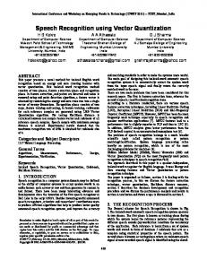
Fig. 2. Viterbi decoder core structure

There are no FPGA cores designed specifically for speech recognition. However, cores do exist for performing Viterbi decoding for signal processing, such as those produced by TILAB and Xilinx. In addition, some DSPs have dedicated logic for Viterbi decoding, for example, the Texas Instruments TMS320C6416 [12], and the TMS320C54x family. In both cases, however, these decoders are designed for signal processing applications, which have different requirements from speech recognition, including narrower data widths, different data formats, and fewer states.

5 System Design The complete system consists of a PC, and an FPGA on a development board inside it. For this implementation, the speech waveforms are processed in advance, in order to extract the observation data used for the decoding. This pre-processing is performed using the HTK speech recognition toolkit [11]. HTK was also used in order to verify the outputs of our system. The speech data is sent to the FPGA, which performs the decoding, outputting the set of most likely predecessor states. This is sent back to the PC, which performs the backtracking process in software. 5.1 FPGA Implementation Structure The structure of the Viterbi decoder core is shown in Fig. 2. This core is virtually identical for both the discrete and continuous HMM versions, differing only in the data widths and the small on-chip data tables. The HMM Block contains the processing elements (or nodes) which compute δt(j). Each node processes the data corresponding to one state of an HMM, as shown in Fig. 3. As every node depends only on data produced by nodes in the previous time frame (i.e. at time t−1), and not the current one, as many nodes can be implemented in parallel as resources and bandwidth allow.

+

δt-1(0)

a0j

ψt(j)

argmin

+

δt-1(1)

min

+

δt(j)

a1j

+

δt-1(2)

a2j

Observation probability bj(Ot) Between-HMM probability (entry state only)

Fig. 3. Node structure

InitSwitch is used at initialisation to set the values of δ0(j). Thereafter,δt(j) is passed to the Scaler, which scales the data in order to reduce the required precision, and discards values which have caused an overflow. In order to keep the design as simple as possible, no language model is being used. As a result, the probability of the most likely transition from any HMM’s exit state to another’s entry state is the same for all HMMs, and is computed and scaled with dedicated blocks as shown. 5.2 Observation Probability Computation The block which computes the observation probabilities for continuous HMMs processes each observation’s 39 elements one at a time, using a fully pipelined architecture. A floating point subtractor, squarer and multiplier are used, with the resulting value sent to an accumulator. The output probability is converted to a fixed point value, and is stored in a FIFO until all of the probabilities corresponding to a single HMM are computed; these values are then sent to the Viterbi decoder core. The observation, mean and variance values are read from off-chip RAM, one of each per clock cycle. However, because the same observation data is used in the calculations for each state, the observation values need only be read in once for each time frame, freeing up part of the data bus for other uses. A buffer stores the values when they are read, then cycles through them for each HMM.

6 Implementation and Results 6.1 System Hardware and Software The design was implemented on a Xilinx Virtex XCV1000 FPGA, sitting on Celoxica’s RC1000-PP development board. The RC1000 is a PCI card, whose features include the FPGA, and 8 Mb of RAM accessible by both it and the host PC. The RC1000 was used within a PC with a Pentium III 450 MHz processor. In order to ensure uniformity of data between HTK and our software and hardware, our software used the same data files as HTK, and produced VHDL code for parts of the design and for testbenches.

6.2 Speech Data The speech waveforms used for the testing and training of both implementations were taken from the TIMIT database [13], a collection of speech data designed for the development of speech recognition systems. Both the test and training groups contained 160 waveforms, consisting of 10 male and 10 female samples from each of 8 American English dialect regions. For these implementations, we used 49 monophone models of 3 states each, with no language model. 6.3 Discrete HMM Implementation For the discrete implementation, the pre-processed speech observations consisted of quantised 8-bit values, treated as addresses into 256-entry, 15-bit-wide look-up tables, one for each state, and stored in off-chip RAM. Internally, scaled probabilities were stored as 16-bit log-domain values, with overflows detected as necessary. The software used the same bit widths. This design was successfully implemented, requiring 1,600 slices, equal to 12% of the XCV1000’s resources. It operated at 55 MHz, with a 62-stage pipeline. Most of this latency was due to the Scaler and between-HMM probability block requiring the data for all 49 HMMs to pass through them before they could produce a result. One consequence of processing just one HMM at a time was that the effective delay due to RAM accesses was reduced, as data from RAM could enter the pipeline as soon as it was read, rather than being buffered first as was done in a previous, more parallel, implementation. Hence a complete observation cycle took 1.13 µs. As the pipeline was circular, all of the HMM data had to pass through it before new data could be processed, but since the pipeline depth was longer than the data length, 11 cycles out of every 62 were wasted. While this implementation had less of a problem with RAM-FPGA bandwidth than more parallel versions, the system had to pause from time to time while predecessor state data was written to RAM. This was aided by queuing the data in the FPGA while it was waiting to be written. A consequence of this was that data was written to RAM continually, including during the cycles wasted while processing was taking place. Taking this into account, the average observation time went up to around 1.8 µs per 10 ms observation - more than 5,500 times real time. 6.4 Continuous HMM Implementation We implemented in software and hardware a continuous HMM-based speech recogniser, which involved computing the observation probabilities as defined in equation (3). As before, the software was written so as to be as functionally similar as possible to the hardware implementation. The continuous observation vectors extracted from the speech waveforms, and the mean and variance vectors for each state, consisted of 39 single-precision floatingpoint values. The observation probabilities calculated from these tended to be one or two orders of magnitude smaller than their discrete HMM counterparts, so it was necessary to increase the fixed point, log-domain, representation from 16 bits to 24.

The design occupied 5,590 of the XCV1000’s slices, equal to 45%, and was capable of running at 47 MHz, though the speed of the off-chip RAM allowed a maximum clock rate of 44 MHz. (We used 1-cycle reads for this implementation, whereas for the discrete one we used 2-cycles reads, allowing a higher clock speed; in both cases, we were limited to using 2-cycle writes). The slowest part of the system was the observation probability computation block, which produced a single value every 40 cycles. Consequently, the Viterbi decoder core sat idle for most of the 133.6 µs which, according to the simulation, the system took to compute all of the observation probabilities for each observation, and then produce the predecessor information. This did at least remove the bottleneck in writing this information to RAM. 6.5 Results The results for the two implementations are shown in Table 1. Time per observation for the hardware is defined as the time between the PC releasing the shared RAM banks after writing the observation data, and the FPGA releasing the banks after writing all the predecessor information. For both implementations, our software and hardware produced the same results as each other, while having a very small number of discrepancies compared to HTK, due to scaling and differences in the representation of data. The times per observation for both hardware implementations are slightly larger than those found from their simulations, probably due to the additional time taken in dealing with the RAM arbitration. The accuracy of these implementations are clearly lower than those found in commercial products (typically above 97%) - but such products use significantly more complex models. It is our intention to move on to more complex models in due course. Comparing the speedups vs. real time for discrete and continuous, the gulf in the hardware speedups is mainly due to the fact that the discrete implementation takes 1 clock cycle to produce 3 observation probabilities in parallel, whereas the continuous one takes 120 clock cycles to do the same. This is not echoed in the software, where we replace serial memory look-ups with floating point calculations. In addition, while the speedup of the discrete HMM hardware implementation over its software counterpart is much higher than for the continuous version, it is likely that future research will focus on continuous HMMs, as for speech recognition, accuracy Table 1. Results from discrete and continuous HMM implementations. Accuracy is (N-D-SI)/N; correctness is (N-D-S)/N; where N is number of phones, and D, S and I are deletion, substitution and insertion errors, respectively

Disc. S/W Disc. H/W Cont. S/W Cont. H/W

FPGA resources 12% 45%

Acc. (%) 28.3 28.3 49.5 49.5

Corr. (%) 31.7 31.7 52.1 52.1

Time/obs (µs) 887 2.03 5390 134

Speedup v S/W 437 40.2

Speedup v real time 11.3 4930 1.86 74.6

takes precedence over speed.

7 Conclusions and Future Work We have implemented a speech recognition system on an FPGA development board, comparing versions based on discrete HMMs and continuous HMMs, and using a simple monophone model. We have demonstrated that both are capable of processing speech data faster than equivalent software, and faster than real time, but that speed has to be sacrificed if greater recognition accuracy is required. The next step is to generate and implement models based on biphones and triphones (combinations of 2 and 3 monophones respectively), which can contain 500 or more HMMs, but result in greater recognition accuracy. As a way of utilising the small amount of spare bandwidth available to the continuous HMM implementation, and the large number of wasted cycles in the decoder core, multiple speech streams could be interleaved within the FPGA. Each one would require its own observation probability computation block, but would share the decoder core.

References 1. Burchard, B. & Romer, R., “A single chip phoneme based HMM speech recognition system for consumer applications,” IEEE Trans. Consumer Elec., 46, No.3, 2000, pp.914-919. 2. Gorin, A.L., Riccardi, G. & Wright, J.H., “How may I help you?” Speech Communication, 23, 1997, pp.113-127. 3. Holmes, J. N. & Holmes WJ, “Speech synthesis and recognition,” Taylor & Francis, 2001 4. Melnikoff, S.J., James-Roxby, P.B., Quigley, S.F. & Russell, M.J., “Reconfigurable computing for speech recognition: preliminary findings,” FPL 2000, LNCS #1896, 2000, pp.495-504. 5. Melnikoff, S.J., Quigley, S.F. & Russell, M.J., “Implementing a hidden Markov model speech recognition system in programmable logic,” FPL 2001, LNCS #2147, 2001, pp.81-90. 6. Nakamura K. et al, “Speech recognition chip for monosyllables,” Proc. Asia and South Pacific Design Automation Conference (ASP-DAC 2001), IEEE, 2001, pp.396-399. 7. Rabiner, L.R., “A tutorial on hidden Markov models and selected applications in speech recognition,” Proceedings of the IEEE, 77, No.2, 1989, pp.257-286. 8. Shi Y.Y., Liu J. & Liu R.S., “Single-chip speech recognition system based on 8051 microcontroller core,” IEEE Trans. Consumer Elec., 47, No.1, 2001, pp.149-153. . 9. Shozakai, M., “Speech interface VLSI for car applications”, ICASSP ’99, 1999, pp.141-144. 10.Stogiannos, P., Dollas, A. & Digalakis, V., “A configurable logic based architecture for realtime continuous speech recognition using hidden Markov models,” Journal of VLSI Signal Processing Systems, 2000, 24, No.2-3, pp.223-240. 11.Woodland, P.C., Odell, J.J., Valtchev, V. & Young, S.J. “Large vocabulary continuous speech recognition using HTK,” ICASSP ’94, 1994, pp.125-128. 12.http://dspvillage.ti.com/docs/dspproducthome.jhtml 13.http://www.ldc.upenn.edu/Catalog/LDC93S1.html 14.http://www.sensoryinc.com/ 15.http://www.speech.philips.com/