SPIKE SORTING WITH SUPPORT VECTOR MACHINES R. Jacob Vogelstein 1 , Kartikeya Murari1 , Pramodsingh H. Thakur1 , Chris Diehl2 , Shantanu Chakrabartty3 , and Gert Cauwenberghs3 1
Department of Biomedical Engineering 2 Applied Physics Labs 3 Department of Electrical and Computer Engineering Johns Hopkins University, Baltimore, Maryland, 21218 {jvogelst,kartik,pramod,gert,shantanu}@jhu.edu,
[email protected] ABSTRACT Spike sorting of neural data from single electrode recordings is a hard problem in machine learning that relies on significant input by human experts. We approach the task of learning to detect and classify spike waveforms in additive noise using two stages of large margin kernel classification and probability regression. Controlled numerical experiments using spike and noise data extracted from neural recordings indicate significant improvements in detection and classification accuracy over linear amplitude- and template-based spike sorting techniques. 1. INTRODUCTION Recording electrical activity from neurons in the brain has become an indispensable technique in modern neuroscience research. Typically, these recordings are obtained by advancing a metal probe through neural tissue until a neuron of interest is located. It is difficult to position an electrode in such a way as to isolate a single neuron, so the activity recorded is frequently derived from multiple neural sources. Unless the contribution of each source can be separated from the others (and from background noise), the integrity of the experiment may be compromised. A number of efforts (reviewed in [1, 2]) have been directed at this problem of neural source separation — commonly called “spike sorting” — but none has been completely effective in all situations. In fact, although new approaches look promising [3]-[6], some of the simplest measures have been most successful [7]. Spike sorting systems rely on the fact that the waveforms (“spikes”) recorded from a specific neuron are functions of both the intrinsic electrochemical dynamics of that neuron and the position of the electrode with respect to the neuron. Furthermore, they assume that in a noiseless system, each recorded spike from a given neuron over a short period of time would be nearly identical, although spikes from different neurons could vary in shape. In reality, though, the system has many sources of noise — slight perturbations in electrode position, activity of distant cells, environmental factors, etc. — and consequently every recorded spike appears different. Moreover, because the spectral contents of spikes and noise are similar, many recorded spikes appear similar to noise, and vice-versa. The ability to distinguish spikes from This work was supported in part by an NSF Graduate Research Fellowship grant to RJV and the NIH Training Program in Neuroengineering #1T32EB003383.
noise (“spike detection”), and to distinguish spikes from different sources (“spike classification”), therefore depends on both the disparities between the noise-free spikes from each source (“templates”) and the signal-to-noise level (SNR) in the recording system. An additional factor that we will not consider as a variable in this paper (but see [3, 8]) is the overall activity level of the neurons, which affects the number of coincident (“overlapping”) spikes. In the following sections we describe a novel spike sorting architecture based on GiniSVM support vector machine classification and probability regression [9]. The spike sorter is evaluated with numerical experiments on spike and noise data extracted from neural recordings over a large range of signal-to-noise ratios and template disparities, and demonstrates superior performance to standard template matching techniques. 2. METHODS 2.1. Experimental Methods Electrophysiology recordings were made in male and female rhesus monkeys (Macaca mulatta), each weighing 4-5 kg, during a sensory neurophysiology experiment. On each recording day, single and multiple units were isolated in cortical areas 1 and 3b using quartz-coated platinum/tungsten (90/10) electrodes (diameter, 80 mm; tip diameter, 4 mm; and impedance, 15 MΩ at 1000 Hz). The raw data were filtered and amplified before being digitized (National Instruments PCI-6052) at a 40 KHz sampling rate and stored. All surgical procedures were done under sterile conditions and in accordance with the rules and regulations of the Johns Hopkins Animal Care and Use Committee and the Society for Neuroscience. During off-line analysis of each recording session, pure noise segments and segments containing putative spikes were automatically identified and manually verified [10, 11]. Putative spike waveforms were time-aligned and clustered in a principal component space under human supervision; templates were formed by averaging all points sufficiently close together. Out of 81 recording sessions, 25 were found to contain two or more templates. 2.2. Data Generation A persistent issue in the spike sorting literature is whether to use real or simulated data to test new algorithms. While using real data would be preferable in some ways, real data is fundamentally
Dataset 16
Dataset 24
Dataset 37
Dataset 55
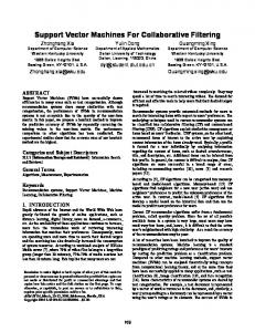
from pure noise segments of real neural recordings (see Section 2.1) and then simulate the noise using an autoregressive filter [13]. Spline-interpolated spike templates (with random phase) are inserted according to a modified Poisson process where the number of spikes in a fixed time period is given by the usual Poisson probability distribution, but the inter-spike interval is not a true exponential random variable because of the refractory period of the neurons. For all of the experiments described below, each simulated recording uses a randomly selected set of noise parameters taken from a real recording session. In order to draw fair comparisons across multiple signal-to-noise ratios, we have selected four representative sets of templates (Figure 1a). After selecting a set of noise statistics and templates for a simulation, we also specify the signal-to-noise ratio (SNR). Although there are many ways of calculating this value, we define it as the root mean squared value of the template divided by the standard deviation of the simulated noise, i.e. SNR = p ktemplatek / σ · |template| where k · k is the L2 norm, σ is the standard deviation of the simulated noise, and | · | is the length in number of samples.
(a) 1
1
SNR=1
1
2.3. Detection and Classification 22
2
SNR=2
1
2 22
2
1
2
2
1
2
SNR=3
1
2
2
1
2
(b) Fig. 1. (a) The four sets of experimentally-recorded templates used in the generative model for all data in this paper. (b) Typical simulated recordings at SNR = 1 (top), SNR = 2 (middle), and SNR = 3 (bottom). Spike locations are labeled with the neuron class.
unlabeled, so it necessitates testing the algorithm using possiblyincorrect labels supplied by a human expert. Therefore, simulated data is used in many spike-sorting publications (e.g. [3, 4, 8, 12]). The lack of standards and publicly-available databases with labeled spikes complicate comparisons between different methods in the published literature. We have created a generative model to simulate a neural recording based on parameters measured from actual recordings, and will gladly provide our simulated data upon request. 2.2.1. Spikes and Noise We simulate a neural recording by inserting real spike templates into a background process of stationary colored Gaussian noise. The background noise process can be completely described by its standard deviation and noise autocorrelation vector. To increase the accuracy of the model, we estimate both of these parameters
The spike sorting system consists of two stages — detection and classification — each trained using a support vector machine (SVM) classifier. The first stage discriminates between noise and the occurrence of a spike over time, and the second stage discriminates between spike templates. GiniSVM [14], a sparse large-margin kernel machine for logistic probability regression, is used to estimate class output probabilities. The class probabilities yield confidence values for the classified spike outputs, and can be used in expectationmaximization based training of partially-labeled data. The quadratic form of entropy in the dual formulation of GiniSVM offers sparsity in the kernel representation, and corresponds to a Huber loss function in the primal formulation [9]. Class probabilities in the binary case take the form P (1|x) =
1 1 P = 1 + e−(wΦ(x)+b) 1 + e−( i yi αi k(x,xi )+b)
(1)
and P (−1|x) = 1−P (1|x), where x is the vector to be classified, xi are training vectors, yi = ±1 are the corresponding class labels, and k(·, ·) defines the kernel. Binary GiniSVM minimizes the following objective function in the dual coefficients αi : X 1X 8γ δij )αj − 4γ αi αi (Qij + α 2 i,j Ci i X subject to yi αi = 0 and 0 ≤ αi ≤ Ci , ∀i min :
(2)
i
where Qij = yi yj k(xi , xj ) is the kernel matrix evaluated at training vectors i and j, γ defines the margin, Ci are (data-dependent) regularization constants, and δij = 1 for i = j and zero otherwise. GiniSVM offers the additional computational advantage that it is compatible with standard quadratic programming techniques for SVM training. For comparison purposes, we also perform spike detection by simple amplitude thresholding and spike classification using a standard template matching technique [2]. For template matching, we average all spikes observed from a given neuron in the SVM
training set and use the mean waveforms as the templates. Decisions are based on the Euclidean distance, Mahalanobis distance, or the distance in a lower-dimensional space defined by principal component analysis, between an input vector and the spike templates (i.e. an input vector is assigned the label of whichever template is closest).
To test the performance of the detection stage, we analyze 10 seconds of simulated stationary neural recordings captured immediately after the initial two seconds used for training the system. A sliding window of 1.25 msec duration is moved across the data and each epoch is evaluated by the SVM. The resulting output is a sequence of probabilities of the given epochs being “spikes” versus “noise”. The performance metric sets a threshold at five times the standard deviation of this signal and calculates merit as the ratio of the difference between hits and false positives to the total number of spikes, where a “hit” is assessed whenever the mean time between successive SVM output threshold crossings occurs within ±0.2 msec of an actual spike time, and a “false positive” is assessed for all mean threshold crossing times outside this range. To test classification performance, we evaluate the fraction of correctly classified spikes in the second stage, assuming correct detection in the first stage. Since the exact spike times are known for the simulated data, we extract 1.25 msec of data beginning from each spike onset and use these as the input to the SVM and template matching algorithms.
Merit
80 60 40 SVM 1 Thresholding
20 0
1
2
3 SNR
4
100 90 80 70 SVM 2 Euclidean Mahalanobis 90% PCA
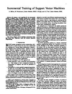
60 3. RESULTS 3.1. Detection Stage For the detection stage, training data is generated from the first two seconds of a simulated neural recording, where each training vector consists of 1.25 msec (50 samples at a 40 KHz sampling rate). Training data include centered spikes as “spike” vectors, surround of spikes as “noise” vectors, and pure noise; 500 examples from each class are used, for a total of 1,500 training vectors. Results from the detection stage are shown in Figure 2a, which plots “merit” (see Section 2.4) against signal-to-noise ratio (SNR). Each point on these lines represents the average performance on ten seconds of simulated data, where averages are taken across all four sets of templates (Figure 1a). For a SNR = 2, the SVM detection stage provides better than 80% accuracy compared to less than 60% for amplitude thresholding, and by SNR = 3 it has reached its asymptotic performance level of about 95%. In comparison, thresholding does not reach an equivalent level until a SNR = 5. The middle axis of Figure 1b shows a recording with SNR = 2 — at this level, the decisions are not obvious to the untrained eye, but the SVM is very effective. For a SNR between zero and one, both basic amplitude thresholding and the SVM detector perform poorly, with a greater number of false positives than correctly classified spike epochs. 3.2. Classification Stage The results of the classification stage, trained over the initial five seconds of data and assuming perfect detection, are summarized in Figure 2b. The SVM classifier consistently outperforms template
5
(a)
Merit
2.4. Performance Measures
100
50 0
2
SNR
4
6
(b) Fig. 2. Performance as a function of SNR for (a) detection stage and (b) classification stage. The “90% PCA” curve illustrates the results if template distance is calculated in a lower-dimensional space where dimensions are chosen to account for approximately 90% of the variance of the data, as given by standard principal component analysis techniques.
matching over the entire range of SNRs tested, although it only exceeds the Euclidean distance metric by a slight margin. Both techniques appear to reach an asymptotic success rate of about 95%. This seems reasonable, as no precautions are taken to avoid simulating overlapping spikes, and destructive interference is likely to render decision making impossible occasionally. Figure 1b provides an example of some typical test data, and Figure 3 illustrates some of the decisions made by the classifier on a SNR = 2 dataset. 4. CONCLUSION We have demonstrated the success of a novel approach to neural spike sorting using support vector machines. For our simulated data, the SVM classifiers outperform standard methods in both the detection and classification stages. Future work will focus on using an expectation maximization-based transductive form of SVM training to deal with nonstationary and partially-labeled data.
tions on Biomedical Engineering, vol. 47, no. 10, pp. 1406– 1411, 2000. [6] Eyal Hulata, Ronen Segev, and Eshel Ben-Jacob, “A method for spike sorting and detection based on wavelet packets and shannon’s mutual information,” Journal of Neuroscience Methods, vol. 117, no. 1, pp. 1–12, 2002. [7] Bruce C. Wheeler and William J. Heetderks, “A comparison of techniques for classification of multiple neural signals,” IEEE Transactions on Biomedical Engineering, vol. 29, pp. 752–759, 1987.
(a)
[8] Michael S. Lewicki, “Bayesian modeling and classification of neural signals,” Neural Computation, vol. 6, no. 5, pp. 1005–1030, 1994. [9] Shantanu Chakrabartty and Gert Cauwenberghs, “Forward decoding kernel machines: A hybrid hmm/svm approach to sequence recognition,” in Proc. of SVM 2002, Seong-Whan Lee and Alessandro Verri, Eds. 2002, pp. 278–292, Springer. [10] Hanzhang Lu, “Neural spike detection and classification,” M.S. thesis, Johns Hopkins University, 1999. [11] Pramodsingh H. Thakur, “Automated optimal detection and classification of neural action potentials in extra-cellular recordings,” M.S. thesis, Johns Hopkins University, 2002.
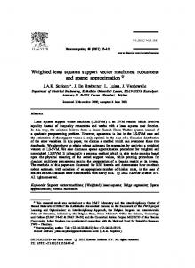
(b) Fig. 3. Sample data from a SNR = 2 dataset determined by the SVM to be (a) class 1 and (b) class 2. Out of the 40 spikes shown here, 3 are misclassified.
5. ACKNOWLEDGMENTS The authors would like to thank Ken Johnson for supervising the work of PHT on the generative model and for his insightful comments regarding this work. 6. REFERENCES [1] Michael S. Lewicki, “A review of methods for spike sorting: the detection and classification of neural action potentials,” Network, vol. 9, pp. R53–R78, 1998. [2] Bruce C. Wheeler, “Automatic discrimination of single units,” in Methods for neural ensemble recordings, M. Nicolelis, Ed., chapter 4, pp. 61–78. CRC Press, Boca Raton, Florida, 1999. [3] Rishi Chandra and Lance M. Optican, “Detection, classification, and superposition resolution of action potentials in multiunit single-channel recordings by an on-line real-time neural network,” IEEE Trans. on Biomed. Engin., vol. 44, no. 5, pp. 403–412, 1997. [4] Karim G. Oweiss and David J. Anderson, “Spike sorting: a novel shift and amplitude invariant technique,” Neurocomputing, vol. 44-46, pp. 1133–1139, 2002. [5] Kyung H. Kim and Sung J. Kim, “Neural spike sorting under nearly 0-db signal-to-noise ratio using nonlinear energy operator and artificial neural-network classifier,” IEEE Transac-
[12] Kerstin M. L. Menne, Andre Folkers, Thomas Malina, Reinoud Maex, and Ulrich G. Hoffman, “Test of spikesorting algorithms on the basis of simulated network data,” Neurocomputing, vol. 44-46, pp. 1119–1126, 2002. [13] George E. P. Box and Gwilym M. Jenkins, Time series analysis: forecasting and control, Holden-Day, Oakland, 1st edition, 1976. [14] Shantanu Chakrabartty and Gert Cauwenberghs, “Forwarddecoding kernel-based phone sequence recognition,” in Advances in Neural Information Processing Systems, Suzanna Becker, Sebastian Thrus, and Klaus Obermayer, Eds., Cambridge, MA, 2003, vol. 15, MIT Press.