Feb 17, 2012 ... Vertex: The fundamental of a network, also called a site (physics), ..... Statistical
Mechanics, P. K. Pathria, Elsevier, 1997 . Statistical Mechanics: ...
Statistical Mechanics of Networks 李明 2011.12.9.
outline • • • • • •
Basic notions of networks(graph) Equilibrium networks Statistical ensembles of networks(graph) Examples and techniques Summary and outlook References
outline • • • • • •
Basic notions of networks(graph) Equilibrium networks Statistical ensembles of networks(graph) Examples and techniques Summary and outlook References
Vertex: The fundamental of a network, also called a site (physics), a node (computer science) , or an actor (sociology). Edge: The line connecting two vertices. Also called a bond (physics), a link (computer science), or a tie (sociology).
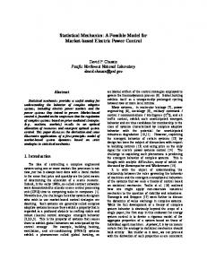
Degree: The number of edges connected to a vertex. A directed graph has both an in-degree and an out-degree for each vertex, which are the numbers of incoming and outgoing edges respectively. k Note that the degree is not necessarily equal to the number of vertices adjacent to a vertex, since there may be more than one edge between any two vertices. (a), (b): tadpole (c): melon Others: hedgehog
Adjacent Matrix Network can be represented in matrix form. A graph of N nodes is described by an N×N adjacent matrix M. Element 𝜍𝑖𝑗 of a adjacent matrix is equal to the number of edges between vertex i and j. Simple relations for an adjacent matrix (1) For undirected graph 𝜍𝑖𝑗 =𝜍𝑗𝑖 (1) The degree of a vertex i is 𝑘𝑖 =
𝜍𝑖𝑗 𝑗
(2) The total degree of the graph 𝐾 = 2𝐿 =
𝑘𝑖 = 𝑖
𝑀2
𝜍𝑖𝑗 = 𝑖𝑗
𝑖𝑖
𝑖𝑖
= 𝑇𝑟 𝑀 2
outline • • • • • •
Basic notions of networks(graph) Equilibrium networks Statistical ensembles of networks(graph) Examples and techniques Summary References
Equilibrium networks Equilibrium networks: the number of vertex N in the network is fixed . Non-equilibrium networks: growing networks, such as BA network.
How to build an equilibrium networks: 1.The random graph model. 2. The configuration model. 3.The hidden variables model.
The random graph model. 1.Uniform model 𝑮𝑵,𝒎 Each graph with m edges has equal
probability
macrostate
?
𝑁 2
𝑚
microstate 2.Binomial model 𝑮𝑵,𝒑 Each possible edge appears independently with probability p 𝑚 =
𝑁 1 𝑝= 𝑁 𝑁−1 𝑝 2 2
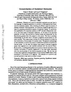
The configuration model. Choosing a degree sequence, which is a set of n values of the degrees k i of vertices i = 1, . . . , n, from this distribution. We can think of this as giving each vertex i in our graph k i “stubs” or “spokes” sticking out of it, which are the ends of edges-to-be. Then choosing pairs of stubs at random from the network and connect them together. As a result, we have a network with a given degree sequence, but otherwise random.
macrostate
𝑘𝑖 = 1,1,2,2,3,4 2
1
6
4 5
3
2
1
?
6
4 5
3
microstate
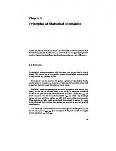
The hidden variables model. (i) To each of the vertex i, ascribe a number — hidden variable di. (ii) Then connect vertices in pairs with probabilities depending on the — hidden variable of these vertices. So that the probability that there is a edge between vertices i and j is 𝑝𝑖𝑗 = 𝑓 𝑑𝑖 , 𝑑𝑗 .
In particular, if 𝑝𝑖𝑗 = 𝑝 is a constant, we arrive at the random graph model.
microstate
?
macrostate
outline • • • • • •
Basic notions of networks(graph) Equilibrium networks Statistical ensembles of networks(graph) Examples and techniques Summary References
Statistical ensembles of networks(graph) A statistical ensemble of graphs is defined by choosing of a set G of graphs and a rule that associates some statistical weight (unnormalized measure) P (g) > 0 with any graph g ∈ G. G can be understand as a set of adjacent matrices. The ensemble average of any quantity A(g) that depends on properties of a graph is 𝑔∈𝐺 𝑃 𝑔 𝐴 𝑔 𝐴 = 𝑍 where Z is a partition function 𝑍=
𝑃 𝑔 𝑔∈𝐺
The Gibbs entropy of the ensembles 𝑆=−
𝑃 𝑔 log 𝑃 𝑔 𝑔∈𝐺
The best choice of probability distribution is the one that maximize the Gibbs entropy subject to the constraints 𝑃 𝑔 𝑥𝑖 𝑔 = 𝑥𝑖
,
𝑃 𝑔 =1
𝐺
Introducing Lagrange multipliers 𝛼, 𝜃𝑖 , 𝛿 − 𝑃 𝑔 log 𝑃 𝑔 + 𝛼 1 − 𝛿𝑃 𝑔 𝐺
Then This gives
𝐺
𝑃 𝑔
+
𝐺
log 𝑃 𝐺 + 1 + 𝛼 +
𝜃𝑖 𝑥𝑖 − 𝑃 𝑔 𝑥𝑖 𝑔 𝐺
𝑖 𝜃𝑖 𝑥𝑖
𝑔 =0
𝑒 −𝐻 𝑔 𝑃 𝑔 = 𝑍 Where 𝐻 𝑔 = 𝑖 𝜃𝑖 𝑥𝑖 𝑔 is the graph Hamiltonian. Z is the partition function 𝑍 = 𝑒 𝛼+1 =
𝑒 −𝐻 𝑔
𝑔
=0
1.Microcanonical ensemble: energy and number of particles are fixed. 2.Canonical ensemble: temperature and number of particles are fixed. 3.Grand canonical ensemble: temperature and chemical potential are fixed.
network(graph)
statistical physic
edge
particle
degree sequence
energy
outline • • • • • •
Basic notions of networks(graph) Equilibrium networks Statistical ensembles of networks(graph) Examples and techniques Summary References
1.Graphs with non-interaction edges We consider the graphs withthe graph Hamiltonian H 𝑔 =
𝜖𝑖𝑗 𝜍𝑖𝑗 𝑔 + 𝑖