Stochastic and Macroscopic Thermodynamics of

PHYSICAL REVIEW X 7, 011008 (2017)

Stochastic and Macroscopic Thermodynamics of Strongly Coupled Systems Christopher Jarzynski1,2,3 1

Institute for Physical Science and Technology, University of Maryland, College Park, Maryland 20742, USA 2 Department of Chemistry and Biochemistry, University of Maryland, College Park, Maryland 20742, USA 3 Department of Physics, University of Maryland, College Park, Maryland 20742, USA (Received 21 September 2016; published 24 January 2017) We develop a thermodynamic framework that describes a classical system of interest S that is strongly coupled to its thermal environment E. Within this framework, seven key thermodynamic quantities— internal energy, entropy, volume, enthalpy, Gibbs free energy, heat, and work—are defined microscopically. These quantities obey thermodynamic relations including both the first and second law, and they satisfy nonequilibrium fluctuation theorems. We additionally impose a macroscopic consistency condition: When S is large, the quantities defined within our framework scale up to their macroscopic counterparts. By satisfying this condition, we demonstrate that a unifying framework can be developed, which encompasses both stochastic thermodynamics at one end, and macroscopic thermodynamics at the other. A central element in our approach is a thermodynamic definition of the volume of the system of interest, which converges to the usual geometric definition when S is large. We also sketch an alternative framework that satisfies the same consistency conditions. The dynamics of the system and environment are modeled using Hamilton’s equations in the full phase space. DOI: 10.1103/PhysRevX.7.011008

Subject Areas: Chemical Physics, Statistical Physics

I. INTRODUCTION Thermodynamics provides a durable conceptual framework for understanding the exchange of matter and energy among macroscopic systems [1–3]. Key elements of this framework include equilibrium states to which systems spontaneously relax, state functions that characterize the properties of equilibrium states, and heat and work— distinct mechanisms for the transfer of energy. The principles of thermodynamics are expressed through a set of postulates or laws, which govern the changes that occur during thermodynamic processes and make predictions about the properties of matter in equilibrium. Despite the dictum that thermodynamics applies only to macroscopic systems, it is hard to deny that nanoscale systems often exhibit thermodynamic-like behavior. Biomolecular motors such as kinesin and myosin are tiny engines that consume chemical energy to produce mechanical work [4]. Just like rubber bands that are stretched and contracted, single strands of RNA exhibit hysteresis and dissipation, in agreement with the second law, when manipulated using optical tweezers [5]. Stochastic thermodynamics [6,7] aims to “scale down” the framework of macroscopic thermodynamics to the level of individual molecules and molecular complexes, as well as mesoscopic

Published by the American Physical Society under the terms of the Creative Commons Attribution 3.0 License. Further distribution of this work must maintain attribution to the author(s) and the published article’s title, journal citation, and DOI.

2160-3308=17=7(1)=011008(20)

systems such as optically trapped micron-size beads. The goal is to formulate a theory that reflects the laws of macroscopic thermodynamics but is applicable to microscopic systems undergoing processes that involve the exchange of energy. A feature that distinguishes microscopic systems is the prominence of fluctuations. While both small and large systems [8] are affected by the thermal motions of their microscopic constituents, in small systems these fluctuations are often appreciable on relevant scales of observation and give rise to statistical fluctuations in the outcomes of experiments [9]. In recent decades, much progress has been made toward incorporating these fluctuations—particularly away from equilibrium—into a broadly applicable thermodynamic framework [6,7,10]. Strong system-environment coupling is another distinctive feature of microscopic thermodynamics. A system S and its environment E are coupled by an interaction energy USE . When S is a macroscopic, three-dimensional body, the system-environment interactions generally occur at its two-dimensional surface and involve only a tiny fraction of its atoms. As a result, the value of USE is negligible in comparison with the internal energy of the system of interest, US , and we can approximate the total energy of the composite system as a sum of subsystem energies: USþE ≈ US þ U E . This partitioning leads directly to the notion of heat—energy lost by E is gained by S, and vice versa—and from there to the first law of thermodynamics. For microscopic systems of interest, the interaction energy cannot be dismissed so easily, as the “surface” of

011008-1

Published by the American Physical Society

CHRISTOPHER JARZYNSKI

PHYS. REV. X 7, 011008 (2017)

S may include most or all of its degrees of freedom. We must then write U SþE ¼ US þ UE þ USE , allowing for USE to be comparable to U S . In this situation, it is not immediately clear whether we should treat U SE as “belonging” to the system of interest or to the environment, or somehow split between the two. If we wish to write down precise statements of the first and second laws of thermodynamics for small systems, this question must be addressed. The aim of this paper is to construct a consistent thermodynamic framework for a system that is strongly coupled to its environment. The framework is built around microscopic definitions of seven key thermodynamic quantities: internal energy, entropy, volume, enthalpy, Gibbs free energy, heat, and work. Temperature and pressure also play a role (of course), but their values are inherited from the environment. We require our framework to satisfy three principles: thermodynamic consistency, stochastic consistency, and macroscopic consistency. Thermodynamic consistency means that the central macroscopic relationships existing among the seven key quantities [Eqs. (1) and (4)] should remain valid for their microscopic counterparts [Eqs. (20) and (21)]. Stochastic consistency means that three important fluctuation theorems should remain valid [Eq. (22)]. Macroscopic consistency means that the definitions of the key quantities should “scale up” properly: Since all seven of these quantities are well defined for macroscopic systems, we demand that when our microscopic definitions are evaluated for a system that happens to be large, the actual macroscopic values will be recovered. A priori, it is not obvious that these conditions can be satisfied. On the contrary, one might naturally expect that finite system-environment coupling would give rise to correction terms in the relationships among thermodynamic quantities, and these terms would become negligible only in the macroscopic limit. However, we show that a consistent framework can be constructed without introducing such correction terms: Eqs. (20)–(22) are exact, for the quantities we define. A number of authors have proposed and investigated precise definitions of thermodynamic quantities for strongly coupled systems [11–17], with Seifert’s approach [15] being the closest in spirit to the present work. In these earlier papers, the condition of macroscopic consistency was not imposed. By demanding this additional condition, we obtain a unifying theoretical framework that defines a consistent stochastic thermodynamics at small length scales and recovers macroscopic thermodynamics at large length scales. Volume plays a central role in this paper. A system’s volume is usually defined geometrically, as a measure of the region of space it occupies. This definition is ambiguous for a microscopic system, which does not possess a sharply defined surface. We instead introduce

a thermodynamic definition: A system’s volume will be defined by its effect on its surroundings [18]. To satisfy macroscopic consistency, this thermodynamic volume must coincide with the geometric volume when the system is large. The plan of the paper is as follows. Section II reviews the relevant macroscopic thermodynamics. Section III introduces the microscopic setup, discusses the equilibrium statistical mechanics of a molecule in solution, and specifies the three consistency criteria mentioned above. Section IV defines the thermodynamic volume of a strongly coupled system. Section V defines the remaining key quantities and shows that they satisfy the desired consistency criteria. Section VI introduces an alternative framework, with different definitions of volume, internal energy, etc. Section VII briefly discusses the tension of a stretched molecule. Section VIII relates our results to others in the literature. We conclude with a discussion in Sec. IX. II. THERMODYNAMICS The general setting considered in this paper involves a system of interest S, a thermal environment E in which that system is immersed, and a work parameter. The system S can be either large (macroscopic) or small (microscopic). In the present section, we consider an ordinary rubber band as an illustrative example, whereas in Sec. III, we consider a single molecule that is manipulated using optical tweezers. The goal is to develop a framework that encompasses both cases. The environment E is macroscopic, vastly larger than the system of interest, and in thermal equilibrium at temperature T and pressure P. In the example considered in this section, E is taken to be a roomful of air surrounding the rubber band. If the system of interest undergoes an irreversible process, then a nearby portion of the environment might temporarily be perturbed away from local equilibrium, but the bulk of the environment is not measurably affected. Although S and E can exchange energy, each contains a fixed number of constituent particles (atoms or molecules). The work parameter is an externally controlled variable (such as the length L of the rubber band) that is used to manipulate the system. An equilibrium state of a macroscopic system is specified by a few state variables. In the case of the rubber band, we take these to be its length L, temperature T, and pressure P. The latter two are defined operationally: The temperature and pressure of the rubber band are equal to those of the environment. A state function is a quantity that has a well-defined value when the system is in equilibrium. For the rubber band, important state functions include the internal energy U, entropy S, tension Ψ, and the volume of space it occupies, V. Each is a function of the state variables, e.g., U ¼ UðL; P; TÞ.

011008-2

STOCHASTIC AND MACROSCOPIC THERMODYNAMICS OF …

  ∂ G H ¼ −T : ∂T T

These state functions are used to define thermodynamic potentials, including the enthalpy H and Gibbs free energy G: H ¼ U þ PV;

G ¼ H − ST:

Q þ W − PΔV ¼ ΔU;

Q ≤ TΔS;

ð2Þ

where Q is the heat absorbed by the rubber band from the surrounding air, Z W ¼ ΨdL ð3Þ is the work associated with varying the length of the rubber band, and ΔV and ΔS denote net changes in volume and entropy. When the rubber band is stretched or contracted, its cross-sectional area changes as well; if the net change is not volume preserving, then the rubber band performs an amount of work PΔV, which may be positive or negative, on the surrounding air. The first and second laws are conveniently expressed using enthalpy and Gibbs free energy: Q þ W ¼ ΔH;

W ≥ ΔG;

ð4Þ

which follow directly from Eqs. (1) and (2). For a reversible process, the inequalities become equalities: Q ¼ TΔS;

W ¼ ΔG:

ð5Þ

Throughout this paper, P and T are viewed as fixed parameters describing a single thermal environment. This implies a one-dimensional manifold of equilibrium states, parametrized by L. Equation (5a) gives the entropy difference between any pair of states in this manifold, thereby defining SðL; P; TÞ up to an additive constant S0 ðP; TÞ. Because the term PΔV is typically negligible in comparison with W and Q, it is generally ignored in discussions of rubber-band thermodynamics; then, ΔH and ΔG in Eq. (4) are replaced by ΔU and ΔF, where F ¼ U − ST is the Helmholtz free energy. Strictly speaking, however, PΔV is a macroscopic quantity (its value is much greater than kB T), which should be included in a precise thermodynamic accounting. More relevantly for present purposes, the analogue of this term plays an important role when the system of interest is microscopic, as we see in Sec. V. The quantities S, V, H, Ψ, and G additionally satisfy [3] ∂G S¼− ; ∂T

∂G V¼ ; ∂P

∂G Ψ¼ : ∂L

2

ð6Þ

Equations (1b) and (6a) imply the Van ’t Hoff equation [19]

ð7Þ

III. STATISTICAL MECHANICS

ð1Þ

At fixed environmental pressure and temperature, the first and second laws of thermodynamics are

PHYS. REV. X 7, 011008 (2017)

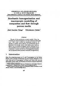
Now consider the setup shown in Fig. 1. A single molecule of RNA, immersed in a macroscopic quantity of water, is tethered between two micron-size polystyrene beads, which in turn are grabbed by a micropipette and a laser trap (optical tweezers). By varying the distance λ, the RNA molecule can be stretched or contracted like a tiny rubber band. We view the molecule and beads as our system of interest S and the surrounding water as a thermal environment E. The water might also include dissolved molecules or ions, so the environment is really an aqueous solution rather than pure water. In Sec. II, the equilibrium state of the rubber band was specified at a thermodynamic level of description. In this section, we take the approach of classical statistical mechanics. The RNA and the two beads are described using n microscopic degrees of freedom, q ¼ ðq1 ; …qn Þ, together with their momenta, p ¼ ðp1 ; …pn Þ. The variable x ¼ ðq; pÞ denotes a point in 2n-dimensional phase space. Similarly, y ¼ ðQ; PÞ denotes a point in the phase space of the aqueous environment, containing the proverbial N ∼ 1023 degrees of freedom. The composite system is governed by a classical Hamiltonian USþE ðx; y; λÞ ¼ uS ðx; λÞ þ U E ðyÞ þ uSE ðx; yÞ:

ð8Þ

Here, uS indicates the bare energy of the system of interest, which depends parametrically on λ, U E is the bare energy of the environment, and uSE is an interaction term. Capital letters will generally denote quantities whose values are macroscopic in magnitude, and lowercase letters will be used for quantities whose values are microscopic. Note that U and u are used here to specify Hamiltonians; the letters H and h are reserved to denote enthalpy. As in Refs. [11,15], we assume that neither UE nor uSE depends on the parameter λ. Thus, variations in λ are coupled directly only to the degrees of freedom of the

FIG. 1. Schematic depiction of single-molecule setup (not to scale). A molecule of RNA attached to two micron-size beads is immersed in aqueous solution and manipulated using optical tweezers. The work parameter λ denotes the distance from the fixed micropipette to the center of the laser trap.

011008-3

CHRISTOPHER JARZYNSKI

PHYS. REV. X 7, 011008 (2017)

system of interest and not to those of the environment. For a model system in which uSE depends on parameters that may be varied with time, see Ref. [20]. In statistical mechanics, we distinguish between “microscopic” and “statistical” states. A microscopic state, or microstate, denotes a single point in phase space, x, and can be viewed as a microscopic snapshot of the system. A statistical state refers to an ensemble of microstates, specified by a probability distribution on phase space, pðxÞ. An equilibrium state is a particular statistical state, represented by a distribution peq α that remains constant in time when the system in question remains undisturbed. An equilibrium state is specified by the values of several fixed parameters, or state variables, α, such as particle number, volume or pressure, and temperature. An observable, or fluctuating observable, is a quantity whose value is determined by the microstate, whereas a state function is a quantity whose value is associated with an equilibrium state. For example, a Hamiltonian uS ðxÞ is a (fluctuating) observable, R eq whereas the equilibrium average uðαÞ ≡ huS ieq ¼ pα ðxÞuS ðxÞ is a state function. The α value uS ðxÞ is the system’s bare internal energy in a particular microstate x, and uðαÞ is its bare internal energy in the equilibrium state α. This example illustrates a convention we follow: A lowercase letter with the subscript S denotes a fluctuating observable; one without the subscript denotes a state function. Although the classification of quantities as fluctuating observables or state functions is sufficient for present purposes, it is not exhaustive [21]. One can construct hybrid quantities that are both functions of the microstate x and functionals of the probability distribution pðxÞ. An example is the self-information R[22] − ln pðxÞ, whose average is the Shannon entropy − p ln p. A. Statistical mechanics of macroscopic systems Statistical mechanics was originally developed to explain how macroscopic thermodynamics emerges from microscopic motions [23–25]. The theoretical framework for describing macroscopic systems in equilibrium is now well established. We recall a few important elements of this framework. Several standard distributions are available to represent macroscopic systems in equilibrium [26]. These include the canonical and isothermal-isobaric distributions 1 −βUðXÞ e ; Z

ð9aÞ

1 −β½UðXÞþPVðXÞ e ; Z

ð9bÞ

peq NVT ðXÞ ¼ peq NPT ðXÞ ¼

as well as the microcanonical, grand canonical, and other distributions. Here, X and UðXÞ denote the microstate and

the Hamiltonian of a generic macroscopic system, Z and Z are partition functions, and β ¼ 1=kB T. The canonical ensemble, Eq. (9a), is defined at fixed system volume, V. In the isothermal-isobaric ensemble, Eq. (9b), the volume is a fluctuating observable, and the factor e−βPV “tunes” the ensemble to a range of volumes determined by the fixed pressure P. Away from phase transitions, this range is macroscopically narrow; hence, the system can be viewed as having a well-defined volume. The Helmholtz and Gibbs free energies corresponding to Eq. (9) are given by FðN; V; TÞ ¼ −β−1 ln Z; GðN; P; TÞ ¼ −β−1 ln Z:

ð10Þ

The equivalence of ensembles asserts that averages computed in the various macroscopic equilibrium ensembles yield the same values. Formally, this equivalence is achieved in the thermodynamic limit of infinitely large systems, and its validity is rooted in the mathematical theory of large deviations [27]. In this paper, we take the thermodynamic limit for the environment (N → ∞), while holding the size of the system of interest (n) fixed, and we define thermodynamic potentials such as enthalpy, entropy, and Gibbs free energy for the system of interest. Thus, we develop a thermodynamic framework for a single small system immersed in a large environment, without invoking the limit n → ∞. B. Solvated ensemble Returning now to the situation depicted in Fig. 1, the equilibrium state of the system of interest S is obtained from that of the composite system S þ E: Z eq p ðxÞ ¼ dyπ eq ðx; yÞ: ð11Þ Here and in the rest of the paper, the letter p denotes a probability distribution in the phase space of the system of interest, and π denotes a probability distribution in the full phase space of the system and environment. By assumption, the aqueous environment is macroscopic, and we will soon take the thermodynamic limit for E while keeping the size of S fixed. It is then reasonable to use one of the standard ensembles discussed in Sec. III A to model the equilibrium state of S þ E. For example, we could model the composite system either at fixed volume [Eq. (9a)] or at fixed pressure [Eq. (9b)]. The equivalence of ensembles suggests that peq ðxÞ does not depend on our choice of ensemble for π eq ðx; yÞ. In other words, we expect that the microcanonical, canonical, isothermal-isobaric, grand, etc. distributions for the macroscopic composite system S þ E, will all lead to the same distribution peq ðxÞ for the microscopic subsystem S, after integrating over the

011008-4

STOCHASTIC AND MACROSCOPIC THERMODYNAMICS OF … environmental degrees of freedom. We are thus free to choose whichever ensemble we find most handy. We use the isothermal-isobaric ensemble to represent the composite system in equilibrium: π eq λNPT ðx; yÞ

1 ¼ expð−β½USþE ðx; y; λÞ þ PV E ðyÞÞ: ð12Þ Yλ

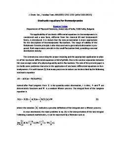
As before, N ∼ 1023 is the total number of particles constituting the thermal environment. To model the PV term [28–31], we add one more degree of freedom to the environment: the fluctuating vertical height h of a piston of mass m that closes off the aqueous solution; see Fig. 2. The volume of the solution is V E ðyÞ ¼ Ah, where A is the crosssectional area of the container. The pressure imposed by the piston is P ¼ mg=A, where g is the gravitational acceleration constant. In this approach, the composite system S þ E is described by a Hamiltonian U tot ðx; y; λÞ ≡ USþE þ PV E ¼ U SþE þ mgh; ð13Þ and Eq. (12) can equally well be interpreted as a canonical distribution, π eq ∝ e−βUtot . From Eqs. (11) and (12), we obtain peq λNPT ðxÞ ¼

1 expð−β½uS ðx; λÞ þ ϕðxÞÞ; Zλ

ð14Þ

where the function ϕðxÞ ¼ ϕðx; N; P; TÞ R dy exp ½−βðU E þ uSE þ PV E Þ −1 R ¼ −β ln dy exp ½−βðUE þ PV E Þ

ð15Þ

is the “solvation Hamiltonian of mean force,” or “solvation Hamiltonian” for short. Note that ϕðxÞ does not depend on the work parameter λ.

FIG. 2. Isothermal-isobaric setup for the RNA molecule in aqueous solution. The container is closed off by a frictionless piston whose vertical height h is treated as one of the many (∼1023 ) degrees of freedom of the environment E.

PHYS. REV. X 7, 011008 (2017)

Taking the thermodynamic limit for the environment, N → ∞, the system of interest becomes a tiny object lost in a vast bath, and ϕ becomes independent of N: ϕðx; P; TÞ ≡ lim ϕðx; N; P; TÞ: N→∞

ð16Þ

In this limit, the equilibrium state of S becomes eq peq λPT ðxÞ ≡ lim pλNPT ðxÞ N→∞

¼

1 expð−β½uS ðx; λÞ þ ϕðx; P; TÞÞ; Zλ

ð17Þ

which is independent of N: The RNA molecule “knows” it is in an aqueous solution at pressure P and temperature T, but it cannot determine whether it is immersed in a droplet of water or in a Great Lake. Throughout the rest of this paper, Eq. (17) will represent the equilibrium state of our system of interest. A few comments are now in order. −βðuS þϕÞ The distribution peq is sometimes called λPT ∝ e “noncanonical” or “non-Gibbsian” because of the term ϕ in the exponent. We instead use the term “solvated ensemble,” emphasizing that Eq. (17) describes a system immersed in an environment of atoms and molecules. Although Eq. (17) was obtained with Fig. 1 in mind, the presumed smallness of S did not enter the derivation. Equation (17) applies equally well when S is macroscopic (e.g., a rubber band), provided the limit N → ∞ is taken for the environment E (the surrounding air), with the size of S held fixed. In that case, x ¼ ðq; pÞ describes a microstate of the rubber band. As we will see in Sec. IV, when S is macroscopic, the value of ϕ reduces to a simple expression. We stress that the choice of the isothermal-isobaric ensemble to represent S þ E [Eq. (12)] was made for convenience. Alternative choices (canonical, microcanonical, grand) would lead to the same solvated ensemble for S, as discussed in greater detail in the Appendix. Both ϕ and peq λPT depend implicitly (through U E þ uSE ) on the chemical composition of the aqueous solution. For instance, ϕðx; P; TÞ is different if E is pure water rather than if it is a solution of water and urea at 8M concentration. This difference is not surprising: The fact that adding urea to water causes proteins to denature (unfold) [32] is empirical evidence that the equilibrium state of a solvated molecule depends not only on the pressure and temperature but also on the chemical composition of its environment. Strictly speaking, we should write ϕðx; P; T; μ1 ; μ2   Þ to indicate the dependence of ϕ on the chemical potentials of the various species of dissolved solutes, but we will leave this dependence implicit. From Eq. (15), we obtain ∂ϕ ðx; λÞ ¼ ∂x

011008-5



∂uSE ∂x

eq x

Z ≡

dyπ eq ðx; yÞ

∂uSE ðx; λÞ: ð18Þ ∂x

CHRISTOPHER JARZYNSKI

PHYS. REV. X 7, 011008 (2017)

Similarly, the quantity hS ≡ uS þ ϕ, which is often called the Hamiltonian of mean force [14–17,33–36], obeys   ∂hS ∂U tot eq : ð19Þ ¼ ∂x ∂x x Thus, −∂ϕ=∂x and −∂hS =∂x are mean values of the fluctuating “forces” −∂uSE =∂x and −∂U tot =∂x, with the average taken over the variables y, at fixed x. Finally, the interaction term uSE often depends only on the coordinates, and not the momenta, of the microscopic degrees of freedom: uSE ¼ uSE ðq; QÞ. In this situation, ϕðxÞ becomes a potential of mean force [37], ϕðqÞ, a concept originally introduced by Kirkwood [38] and widely used in solvation thermodynamics [39]. C. The task at hand Having determined the equilibrium state peq λPT ðxÞ, we wish to define the following state functions for the system of interest: internal energy u, entropy s, volume v, enthalpy h, and Gibbs free energy g. We also wish to define the work w performed on S, and the heat q absorbed by S, during a thermodynamic process in which the system evolves in time. These quantities will be constructed to satisfy three consistency criteria, described below. (1) Thermodynamic consistency requires that these quantities satisfy the analogues of Eqs. (1) and (4): h ¼ u þ Pv;

g ¼ h − sT;

hqi þ hwi ¼ Δh;

hwi ≥ Δg:

ð20Þ ð21Þ

Equation (21) applies to a process in which the system evolves from one equilibrium state to another, Δh and Δg denote the enthalpy and Gibbs free energy differences between these equilibrium states, and angular brackets indicate an average over an ensemble of realizations (repetitions) of this process. (2) Stochastic consistency demands that three central nonequilibrium work relations [10] be satisfied: he−βw i ¼ e−βΔg ; ρF ðþwÞ ¼ eβðw−ΔgÞ ; ρR ð−wÞ hδðx − xt Þe−βwt i ¼ e−βΔgt peq λt ðxÞ:

ð22aÞ ð22bÞ ð22cÞ

These will be described in detail in Sec. V D. These relations were originally derived using the canonical ensemble for the system’s equilibrium state [40–42]. As a result, they are typically expressed in terms of the Helmholtz free-energy difference ΔF, rather than Δg. (3) Macroscopic consistency requires that the state functions u, s, v, h, and g scale up properly. Since

a rubber band surrounded by air can be described using Eqs. (8) and (17), the definitions of u, s, v, etc., which we aim to construct, can, in principle, be evaluated for the rubber band. We want these values to be equal to the macroscopic internal energy, entropy, volume, etc. of the rubber band. Furthermore, w and q can be evaluated for a process involving the stretching or contraction of the rubber band. We want our microscopic expressions for w and q to reproduce the macroscopic work and heat. IV. MICROSCOPIC VOLUME We now introduce a thermodynamic definition of the volume of our microscopic system of interest, both as a fluctuating observable vS ðxÞ and as a state function vðλÞ [Eq. (28)]. Many quantities discussed in this section, including vS and v, depend parametrically on the pressure P and temperature T of the environment. To avoid clutter, we will mostly leave the dependence on P and T implicit. In Eq. (15), the quantity inside the logarithm can be viewed as a ratio of partition functions. The numerator Z E Z x ≡ dy exp ½−βðU E þ uSE þ PV E Þ ð23Þ corresponds to an equilibrium state of E in which the RNA and beads have been inserted into the water, in a “frozen” microstate x; i.e., the system coordinates and momenta x ¼ ðq; pÞ are treated as fixed parameters, rather than degrees of freedom. The denominator, Z E Z 0 ≡ dy exp ½−βðU E þ PV E Þ; ð24Þ is the partition function for an equilibrium state of the bare environment. The solvation Hamiltonian ϕðxÞ ¼ −β−1 ln ðZ Ex =Z E0 Þ ¼ GEx − GE0

ð25Þ

is the Gibbs free-energy difference between these states. This difference is the reversible work associated with “turning on” the interaction between the system of interest—frozen in the microstate x—and the surrounding aqueous solution, at fixed pressure and temperature. In other words, ϕðxÞ is the reversible work required to insert the frozen system of interest into the solution. Suppose for a moment that the system of interest is macroscopic, though much smaller than the environment. For instance, imagine a pebble (S) in a bucket of water (E). Let x denote the positions and momenta of all of the atoms that compose the pebble, and let V peb ðxÞ denote the macroscopic volume of space occupied by the pebble. Note that once the microstate x is given, the macroscopic volume V peb ðxÞ is fully specified. (This is equally true for a squishier system such as a rubber band.)

011008-6

STOCHASTIC AND MACROSCOPIC THERMODYNAMICS OF … Consider the two equilibrium states of the environment depicted in Fig. 3. The state on the left contains only the water, and the state on the right contains the pebble, frozen in the microstate x. The Gibbs free-energy difference between these two states is the reversible work required to grow a cavity of just the right size to accommodate the pebble. Since the pebble is macroscopic, the creation of this cavity requires work PV peb against the fixed pressure P. We therefore have ϕðx; P; TÞ ¼ PV peb ðxÞ:

ð26Þ

1 −β½uS ðx;λÞþPvS ðxÞ e ; Zλ Z Z λ ðP; TÞ ¼ dxe−βðuS þPvS Þ :

peq λPT ðxÞ ¼

ϕðxÞ ; P

ð27Þ

ð28aÞ

Z vðλÞ ≡

dxpeq λ ðxÞvS ðxÞ:

ð30Þ

V. BARE REPRESENTATION

This can be viewed as a thermodynamic definition of volume. The frozen pebble’s volume is given in terms of the work required to insert it into a bath of water. The same argument could have been made for a generic macroscopic system, such as a rubber band (S) in a roomful of air (E), yielding the same result. Since a microscopic system such as our solvated RNA molecule does not possess a sharply defined surface, it is difficult to specify with precision its geometric volume. By contrast, the solvation Hamiltonian ϕðx; P; TÞ is well defined. Motivated by Eq. (27), we define the volume of a microscopic system in terms of its thermodynamic effect on the surrounding environment. Let the fluctuating observable vS ðx; P; TÞ denote the volume of the system of interest in a microstate x; let the state function vðλ; P; TÞ be the volume associated with the equilibrium state ðλ; P; TÞ. We define these as follows (suppressing their dependence on P and T): vS ðxÞ ≡

ð29Þ

Equation (29) resembles the isothermal-isobaric distribution, Eq. (9b), which is intuitively appealing: If the system of interest is immersed in an environment at fixed pressure and temperature, and its volume vS can fluctuate, then it is natural for the isothermal-isobaric ensemble to describe the equilibrium state of the system.

Equation (26) trivially implies ϕðx; P; TÞ V peb ðxÞ ¼ : P

PHYS. REV. X 7, 011008 (2017)

ð28bÞ

Equation (28) defines the volume of a small, solvated system of interest. Here, we define the six remaining quantities (internal energy, entropy, etc.), and we show that they satisfy thermodynamic, stochastic, and macroscopic consistency. The framework developed in this section will be called the bare representation because the internal energy of S will be identified with its bare Hamiltonian, uS [Eq. (31a)]. In Sec. VI, we develop an alternative framework, the partial molar representation. Table I lists the quantities defined in the two frameworks. A. Fluctuating observables and state functions In the bare representation, we define the fluctuating internal energy, volume, and enthalpy of S as follows: internal energy ¼ uS ðx; λÞ; volume ¼ vS ðxÞ ¼

ð31aÞ ϕ ; P

enthalpy ¼ hS ðx; λÞ ¼ uS þ PvS :

ð31bÞ ð31cÞ

Note that the fluctuating volume vS ðxÞ, like the solvation Hamiltonian ϕðxÞ, does not depend on λ. Using the distribution peq λ ðxÞ [Eq. (17)], we construct the state functions Z uðλ; P; TÞ ¼ dxpeq ð32aÞ λ ðxÞuS ðx; λÞ;

Equation (17) can now be written as

Z vðλ; P; TÞ ¼

dxpeq λ ðxÞvS ðxÞ;

ð32bÞ

dxpeq λ ðxÞhS ðx; λÞ;

ð32cÞ

eq dxpeq λ ðxÞ ln pλ ðxÞ;

ð32dÞ

Z hðλ; P; TÞ ¼ Z sðλ; P; TÞ ¼ − FIG. 3. The reversible work required to insert a pebble into a bucket of water, at constant pressure, is PV peb .

011008-7

gðλ; P; TÞ ¼ −β−1 ln Z λ :

ð32eÞ

CHRISTOPHER JARZYNSKI

PHYS. REV. X 7, 011008 (2017)

TABLE I. Thermodynamic quantities defined in the bare and partial molar representations are listed, together with references to their ¯ etc.) All of defining equations. Although w ¼ w¯ and g ¼ g¯ , other quantities generally differ in the two representations (uS ≠ u¯ S , q ≠ q, the listed quantities depend implicitly on P and T. Bare representation Fluctuating observables

Internal energy Volume Enthalpy Internal energy Volume Enthalpy Entropy Gibbs free energy Heat Work

State functions

uS ðx; λÞ vS ðxÞ hS ðx; λÞ uðλÞ vðλÞ hðλÞ sðλÞ gðλÞ q½xðtÞ; λðtÞ w½xðtÞ; λðtÞ

Equation (28b) has been repeated, and Z λ is given by Eq. (30). The internal energy, volume, and enthalpy state functions are defined as equilibrium averages of the respective fluctuating observables [Eqs. (32a)–(32c)], the entropy is given by the Shannon formula [Eq. (32d)], and the Gibbs free energy is defined in terms of a partition function [Eq. (32e)], as in Eq. (10). For every equilibrium state ðλ; P; TÞ of the system of interest, Eq. (32) assigns a unique value to each of these five observables. B. Heat and work Now consider a process in which the composite system S þ E evolves over a time interval ti ≤ t ≤ tf . The work parameter is varied according to a schedule, or protocol, λðtÞ, and the evolution of S is described by a trajectory xðtÞ. Let xi , xf , λi , and λf denote the initial and final microstates and parameter values, e.g., xi ¼ xðti Þ. For a macroscopic system undergoing an isobaric process, the first law is conveniently written as [see Eq. (4)] ΔH ¼ Q þ W:

ð33Þ

The total work performed on the system consists of the work W due to the manipulation of external parameters and the work −PΔV associated with the change of the system’s volume during the process. The latter is sometimes called the “PdV work” and the former the “non-PdV work.” In Eq. (33), the PdV work is bundled into the enthalpy change, ΔH ¼ ΔU þ PΔV (see Sec. II). Motivated by Eq. (33), we write ΔhS ≡ hS ðxf ; λf Þ − hS ðxi ; λi Þ ¼ q þ w;

ð34Þ

where Z q½xðtÞ ≡

ti

tf

dt_x

∂hS ; ∂x

ð35aÞ

Eq. Eq. Eq. Eq. Eq. Eq. Eq. Eq. Eq. Eq.

Partial molar representation

(31a) (31b) (31c) (32a) (32b) (32c) (32d) (32e) (35a) (35b)

u¯ S ðx; λÞ v¯ S ðxÞ h¯ S ðx; λÞ ¯ uðλÞ ¯ vðλÞ ¯ hðλÞ s¯ ðλÞ g¯ ðλÞ ¯ q½xðtÞ; λðtÞ ¯ w½xðtÞ; λðtÞ

Z w½xðtÞ ≡

ti

tf

dtλ_

Eq. Eq. Eq. Eq. Eq. Eq. Eq. Eq. Eq. Eq.

∂hS : ∂λ

(78a) (75) (78b) (80a) (80b) (80c) (83) (83) (85a) (85b)

ð35bÞ

The integrands are evaluated along the trajectory xðtÞ and the protocol λðtÞ (the dependence on the latter is implicit), with x_ ¼ dx=dt and λ_ ¼ dλ=dt. To interpret these definitions, consider first a process with λ held fixed. For example, imagine a protein molecule undergoing a spontaneous conformational change from an unfolded state at t ¼ ti to a compact, folded state at t ¼ tf . From Eqs. (34) and (35), we have q ¼ ΔhS ¼ ΔuS þ PΔvS ;

when λ_ ¼ 0:

ð36Þ

When a macroscopic system undergoes a spontaneous process at constant pressure, the heat that it absorbs is equal to the change in its enthalpy [19]; Eq. (36) is the microscopic analogue of this statement. The term PΔvS represents the PdV work performed by the molecule as it folds spontaneously. From Eq. (31), we have ∂ λ hS ¼ ∂ λ uS (since ∂ λ vS ¼ 0); hence, Eq. (35b) coincides with the accepted definition of work in stochastic thermodynamics [6,7]. This quantity represents non-PdV work: It is associated with variations of the work parameter λ (see also Sec. VII). Thus, Eq. (34) can be rewritten as ΔuS ¼ q þ w − PΔvS ¼ q þ wnon-PdV þ wPdV :

ð37Þ

When a molecule is stretched using optical tweezers, from a folded to an unfolded state, wnon-PdV ¼ w is the work due to the displacement of the optical trap, and wPdV ¼ −PΔvS is the work associated with the change in volume vS that accompanies this process. We interpret Eqs. (34) and (37) as statements of the first law of thermodynamics, for a single realization of a process involving a small system S immersed in a large environment E.

011008-8

STOCHASTIC AND MACROSCOPIC THERMODYNAMICS OF …

  ∂hS eq _ w½xðtÞ → dtλ ∂λ ti Z B Z ∂hS ¼ dλ dxpeq ðx; λÞ λ ðxÞ ∂λ A Z B ∂g ¼ dλ ¼ gðBÞ − gðAÞ ≡ Δg; ∂λ A Z

C. Thermodynamic consistency With the help of Eqs. (31c) and (32e), Eq. (29) becomes peq λ ¼ exp½−βðhS − gÞ:

ð38Þ

This expression combines with Eqs. (32c) and (32d) to give s ¼ βðh − gÞ, or g ¼ h − sT:

ð39aÞ

tf

q½xðtÞ ¼ hS ðxf ; BÞ − hS ðxi ; AÞ − Δg: ð39bÞ

Thus, the first two conditions of thermodynamic consistency identified in Sec. III C [Eq. (20)] are satisfied. Now consider a process in which S begins in equilibrium at λ ¼ A, then the parameter is varied with time (perhaps slowly, perhaps not) until it reaches a final value λ ¼ B, and the system is then allowed to relax to the corresponding equilibrium state [43]. Equation (34) gives us

ð44Þ

using the definitions of hS and g. Equations (34) and (44) give us

Moreover, Eqs. (31c) and (32a)–(32c) imply h ¼ u þ Pv:

PHYS. REV. X 7, 011008 (2017)

ð45Þ

Averaging both sides over an ensemble of realizations of this quasistatic process, the right side becomes Δh − Δg, which combines with Eq. (39a) to give hqi ¼ TΔs:

ð46Þ

This is the Clausius equality for reversible, isothermal processes. D. Stochastic consistency

q þ w ¼ hS ðxf ; BÞ − hS ðxi ; AÞ:

ð40Þ

Averaging both sides over an ensemble of realizations of this process and using Eq. (32c), we get hqi þ hwi ¼ hðBÞ − hðAÞ ¼ Δh

ð41Þ

using the assumption that the system begins and ends in equilibrium. Thus, the third condition of thermodynamic consistency [Eq. (21a)] is satisfied. In Sec. V D, we show that the equality he−βw i ¼ e−βΔg is satisfied for the process described in the previous paragraph [Eq. (52)]. By Jensen’s inequality (see Ref. [37], Sec. V. 5), this result immediately implies that hwi ≥ Δg;

ð42Þ

thereby satisfying the fourth and final condition of thermodynamic consistency [Eq. (21b)]. Using Eqs. (39a) and (41), Eq. (42) can be rewritten as hqi ≤ TΔs;

ð43Þ

which is the Clausius inequality for isothermal processes. It is useful to analyze a scenario in which the system is driven quasistatically from λi ¼ A to λf ¼ B, remaining in equilibrium at all times. In other words, the statistical state of S at time t is given by peq λðtÞ ðxÞ [Eq. (29)]. In this limit, we use adiabatic averaging to replace the integrand in Eq. (35b) with its equilibrium average:

Stochastic thermodynamics provides an appealing framework for deriving and interpreting fluctuation theorems [7]. In this approach, the system of interest evolves under stochastic, Markovian dynamics. The source of stochasticity is a thermal environment whose degrees of freedom are not treated explicitly. An alternative approach is to use Hamilton’s equations to describe the evolution of either the system of interest itself (if it is thermally isolated) or the system and its environment. Simple derivations of counterparts of Eqs. (22a)–(22c) above were presented in Ref. [10] for a toy model of an isolated classical system obeying Hamiltonian dynamics. These derivations were meant to be pedagogical, but they are easily extended to the case of a system that is strongly coupled to its thermal environment. The key is to combine Hamiltonian dynamics in the full phase space (S þ E) with a useful factorization of partition functions [Eq. (50) below]. This approach was previously used in Refs. [11,15], and it is the approach we will follow below. The Hamiltonian for the combined system of interest and thermal environment is given by Utot ðζ; λÞ ¼ uS ðx; λÞ þ UE ðyÞ þ uSE ðx; yÞ þ PV E ðyÞ; ð47Þ where ζ ¼ ðx; yÞ and PV E ðyÞ ¼ mgh [see Eq. (13)]. We assume time-reversal invariance,

011008-9

U tot ðζ; λÞ ¼ U tot ðζ ; λÞ;

ð48Þ

CHRISTOPHER JARZYNSKI

PHYS. REV. X 7, 011008 (2017)

where ζ  is obtained from ζ by reversing all the momenta. This assumption will be used in the derivation of Eq. (22a). At fixed λ, the equilibrium state of S þ E is described by the distribution [see Eq. (12)] π eq λ ðζÞ ¼

1 −βUtot ðζ;λÞ 1 −βðUSþE þPV E Þ e ¼ e : Yλ Yλ

ð49Þ

The dependence of π eq λ and Y λ on ðN; P; TÞ is suppressed. Using Eqs. (23)–(25) and (30), we obtain Z Z −βUtot Y λ ¼ dζe ¼ dxe−βuS ðx;λÞ Z Ex ¼ Z λ Z E0 : ð50Þ Thus, the composite partition function (Y λ ) is a product of partition functions for the system of interest (Z λ ) and the bare environment (Z E0 ). A similar factorization arises in the canonical—rather than isothermal-isobaric—setting [11,12,14–17,33,34]. Now imagine that the composite system begins in equilibrium at t ¼ 0, with λ0 ¼ A; then it evolves in time as the work parameter is varied from λ0 ¼ A to λτ ¼ B according to a protocol λt ≡ λðtÞ. We assume this evolution follows Hamilton’s equations in the full phase space. For a given realization of this process, let ζt ≡ ζðtÞ denote the Hamiltonian trajectory followed by the composite system, and xt ≡ xðtÞ the trajectory of the system of interest, obtained by projecting ζt onto x space. We then have Z τ Z τ ∂hS ∂Utot _ w¼ dtλ dtλ_ ðxt ; λt Þ ¼ ðζt ; λt Þ ∂λ ∂λ 0 Z0 τ d ¼ dt Utot ðζt ; λt Þ ¼ Utot ðζ τ ; BÞ − Utot ðζ0 ; AÞ ð51Þ dt 0 using the Hamiltonian identity dUtot =dt ¼ ∂U tot =∂t (Ref. [44], Sec. 8-2). Note that w can be viewed either as a functional of the entire trajectory xt of the system of interest [Eq. (35b)] or as a functional of the trajectory ζt of the composite system, in which case it is determined directly from ζ 0 and ζ τ [Eq. (51)]. With these elements in place, we have Z −βw −βw½ζ t  he i ¼ dζ0 π eq A ðζ 0 Þe Z ¼

dζ0 Z

e−βUtot ðζ0 ;AÞ −β½Utot ðζτ ;BÞ−Utot ðζ0 ;AÞ e YA    ∂ζ τ −1   e−βUtot ðζτ ;BÞ dζτ  ∂ζ 

1 ¼ YA 0 YB ZB ¼ ¼ ¼ e−βΔg : YA ZA

Next, consider the setup associated with Crooks fluctuation theorem [41,45]. The term “forward process” indicates the situation discussed above, with the work parameter varied from λF0 ¼ A to λFτ ¼ B. The term “reverse process” indicates the time-reversed protocol: λRt ¼ λFτ−t . Initial conditions are sampled from the approeq priate equilibrium distribution, π eq A or π B , and the dynamics are Hamiltonian in the full phase space. Since Utot ðζ; λÞ satisfies time-reversal invariance [Eq. (48)], realizations of the two processes come in pairs, or conjugate twins, F ζFt ¼ ζ R τ−t . Here, ½ζ t  is a solution of Hamilton’s equations for the forward process, and ½ζRt  is the solution for the reverse process obtained by running the forward realization backward in time, so to speak [10,46]. From Eqs. (48) and (51), we have w½ζFt  ¼ −w½ζ Rt :

ð53Þ

Because the dynamics are deterministic, the probability of observing a given trajectory can be equated with that of sampling its initial conditions. Writing PF ½ζFt  as the probability to observe the trajectory ½ζ Ft  during the forward process, and PR ½ζRt  as the probability of observing its conjugate twin during the reverse process, we have F F PF ½ζ Ft  π eq π eq A ðζ 0 Þ A ðζ 0 Þ ¼ ¼ R F PR ½ζ Rt  π eq π eq B ðζ 0 Þ B ðζ τ Þ Y F F ¼ B eβ½Utot ðζτ ;BÞ−Utot ðζ0 ;AÞ YA

¼ eβðw−ΔgÞ ;

ð54Þ

where w ¼ w½ζFt  is the work performed during the forward process. Using Eq. (54), we now obtain Z F ρ ðwÞ ¼ dζF0 PF ½ζ Ft δðw − w½ζ Ft Þ Z ¼ dζR0 PR ½ζRt eβðw−ΔgÞ δðw − w½ζFt Þ Z βðw−ΔgÞ ¼e dζ R0 PR ½ζRt δðw þ w½ζ Rt Þ ¼ eβðw−ΔgÞ ρR ð−wÞ

ð55Þ

using the conjugate pairing of trajectories to replace dζ F0 by dζ R0 . We thus obtain Crooks fluctuation theorem: ρF ðþwÞ ¼ eβðw−ΔgÞ : ρR ð−wÞ

ð52Þ

The first three lines here follow the derivation given in Sec. III of Ref. [10], invoking Liouville’s theorem to set the Jacobian j∂ζτ =∂ζ0 j to unity. Equations (50) and (32e) have been used on the last line.

ð56Þ

Finally, to obtain Eq. (22c), consider

011008-10

χðζ; tÞ ≡ hδðζ − ζt Þe−βwt i

ð57Þ

STOCHASTIC AND MACROSCOPIC THERMODYNAMICS OF … where ζt denotes the microstate of the composite system at time t during a single realization of the forward process, wt is the work performed up to time t during this realization, and angular brackets denote an average over an ensemble of realizations, with initial conditions sampled from π eq A ðζ 0 Þ. The function χðζ; tÞ is a “weighted” probability distribution in the full phase space, in which each realization carries a time-dependent statistical weight expð−βwt Þ [47]. Following the derivation appearing in Eqs. (22)–(26) of Ref. [10], we obtain hδðζ − ζt Þe−βwt i ¼

1 −βUtot ðζ;λt Þ e : YA

ð58Þ

Integrating both sides with respect to y then gives us 1 −βuS ðx;λt Þ E e Zx YA 1 −β½uS ðx;λt ÞþPvS ðxÞ ¼ e ZA

shows that this result holds as well for a system that is strongly coupled to a thermal environment, with −βðuS þϕÞ peq . λ ∝e E. Macroscopic consistency To establish macroscopic consistency, we use the rubber band introduced in Sec. II as an illustrative system. The equilibrium state of the rubber band (immersed in air) is described by peq LPT ðxÞ [Eq. (17)], where x denotes its microstate, and the externally controlled length L plays the role of the work parameter λ. Let the fluctuating observable V S ðxÞ denote the geometric volume of the rubber band. From the arguments leading to Eq. (26), we have ϕðx; P; TÞ ¼ PV S ðxÞ; hence, vS ðx; P; TÞ ≡

hδðx − xt Þe−βwt i ¼

ð59Þ

using Eqs. (23), (25), (28a), and (50). Equivalently, hδðx − xt Þe−βwt i ¼ e−βΔgt peq λt ðxÞ;

ð60Þ

where Δgt ¼ gðλt Þ − gðAÞ. By the simple trick of assigning a weight expð−βwt Þ to each trajectory, we reconstruct the solvated ensemble peq λt ðxÞ (up to normalization) from an out-of-equilibrium ensemble. Since the right side of Eq. (54) can be determined from the trajectory ½xt  alone, we can equally well write PF ½xFt  ¼ eβðw−ΔgÞ ; PR ½xRt 

w ¼ w½xFt ;

ð61Þ

where ½xFt  and ½xRt  are conjugate twin trajectories of the system of interest: xFt ¼ xR τ−t . The numerator (and denominator) in Eq. (61) can be written in the form F PF ½xFt  ¼ PF ½xFt jxF0 Þ · peq A ðx0 Þ;

ð62Þ

where PF ½xFt jxF0 Þ is the conditional probability of observing the trajectory, given the initial conditions. Using Eqs. (29), (32e), and (34), we then obtain PF ½xFt jxF0 Þ ¼ e−βq ; PR ½xRt jxR0 Þ

PHYS. REV. X 7, 011008 (2017)

ð64Þ

For a macroscopic system, the “thermodynamic” volume vS loses its dependence on P and T and becomes equal to the geometric volume V S . Fluctuations in V S ðxÞ among microstates sampled from peq LPT ðxÞ are negligible at the macroscopic scale. As a result, the equilibrium state function V can be equated with the ensemble average of V S ðxÞ: Z VðL; P; TÞ ≡ dxpeq ð65Þ LPT ðxÞV S ðxÞ ¼ vðL; P; TÞ using Eqs. (64) and (32b). The rubber band’s internal energy U S is a sum of the energies of its microscopic constituents, including the interactions among these constituents. This sum is given by the bare system Hamiltonian uS : US ðx; LÞ ¼ uS ðx; LÞ:

ð66Þ

Since fluctuations in US ðx; LÞ within the ensemble peq LPT ðxÞ are macroscopically negligible, we identify the equilibrium energy with its ensemble average: Z UðL; P; TÞ ≡ dxpeq ð67Þ LPT ðxÞU S ðx; LÞ ¼ uðL; P; TÞ: Similar expressions for enthalpy follow immediately: HS ðx; LÞ ¼ U S þ PV S ¼ hS ðx; L; P; TÞ;

ð63Þ

ð68Þ

Z HðL; P; TÞ ¼

q½xFt 

where q ¼ is the heat absorbed by S during the forward process [Eq. (35a)]. The original version of this result—for a system represented in equilibrium by −βuS peq —was obtained by Crooks [41] using disλ ∝e crete-state Markovian dynamics, and extended by Seifert [48] to overdamped Langevin dynamics. Equation (63)

ϕðx; P; TÞ ¼ V S ðxÞ: P

peq LPT H S ¼ hðL; P; TÞ:

ð69Þ

We see that the state functions u, v, and h defined in Eq. (32) scale up to the macroscopic internal energy (U), volume (V), and enthalpy (H). Moreover, the solvated ensemble [Eq. (17)] scales up to the macroscopic isothermal-isobaric ensemble [Eq. (9a)]:

011008-11

CHRISTOPHER JARZYNSKI peq LPT ðxÞ ¼

1 −β½US ðx;LÞþPV S ðxÞ e : ZL

PHYS. REV. X 7, 011008 (2017) ð70Þ

Now consider work and heat. Imagine that the air (E) and rubber band (S) are located within a container, closed off by a piston that maintains a constant pressure. The entire setup constitutes a large, thermally isolated system governed by the Hamiltonian U tot ðζ; λÞ [Eq. (47)]. The macroscopic work performed when stretching the rubber band, W, is equal in value to the total change in the energy of this isolated system. By Eq. (51), this change is equal to the work w defined by Eq. (35b): W ¼ Utot ðζ τ ; BÞ − Utot ðζ0 ; AÞ ¼ w:

ð72Þ

using the first law of thermodynamics [Eq. (4a)]. Equations (71) and (72) establish the macroscopic consistency of w and q. Next, imagine that the rubber band is stretched or contracted slowly, always remaining in equilibrium with the air. Let Δs denote the net change in the state function s [Eq. (32d)], and let ΔS denote the net change in the macroscopic entropy. We then have hqi hQi Δs ¼ ¼ ¼ ΔS T T

v¯ S ðxÞ ¼ V Ex − V E0 ;

ð73Þ

V Ex

The definition of volume introduced in Sec. IV was motivated by the equation V peb ¼ ϕ=P [Eq. (27)]. However, using Eq. (26), we could just as easily have written ∂ϕ V peb ðxÞ ¼ ðx; P; TÞ: ∂P

1 ≡ E Zx

V E0 ≡

Z

1 Z E0

Z

dyV E ðyÞe−βðUE þPV E Þ :

ð77bÞ

ð78aÞ

h¯ S ðx; λ; P; TÞ ≡ H Ex − HE0 ¼ u¯ S þ P¯vS ;

ð78bÞ

where UEx ≡ U E0

1 Z Ex

1 ≡ E Z0

Z Z

dyUSþE e−βðUE þuSE þPV E Þ ;

ð79aÞ

dyU E e−βðUE þPV E Þ ;

ð79bÞ

HEx ≡ UEx þ PV Ex ;

HE0 ≡ UE0 þ PV E0 :

ð79cÞ

We now use the equilibrium averages of u¯ S , v¯ S , and h¯ S to define the corresponding state functions: Z ¯ P; TÞ ≡ uðλ;

¯ S ðx; λ; P; TÞ; dxpeq λ ðxÞu

ð80aÞ

dxpeq vS ðx; P; TÞ; λ ðxÞ¯

ð80bÞ

¯ dxpeq λ ðxÞhS ðx; λ; P; TÞ:

ð80cÞ

Z ð74Þ

This observation suggests an alternative definition of microscopic volume as a fluctuating observable:

¯ P; TÞ ≡ hðλ;

∂ϕ ðx; P; TÞ: ∂P

ð77aÞ

u¯ S ðx; λ; P; TÞ ≡ UEx − U E0 ;

v¯ ðλ; P; TÞ ≡

v¯ S ðx; P; TÞ ≡

dyV E ðyÞe−βðUE þuSE þPV E Þ ;

Here, V E ðyÞ ¼ Ah is the fluctuating volume of the solution (Sec. III B); V E0 is the equilibrium average value of this volume, in the absence of the system of interest; and V Ex is the equilibrium volume of the solution in the presence of the system of interest, frozen in microstate x. Thus, v¯ S ðxÞ is the change in the equilibrium volume of the solution, upon reversibly inserting the frozen system of interest into the environment. Let us define internal energy and enthalpy analogously:

using Eqs. (46), (72), and (5a). Since SðLÞ is defined only up to an additive constant S0 (see Sec. II), we conclude from Eq. (73) that s ¼ S. Finally, since h and s scale up to their macroscopic counterparts H and S, and since we have already established g ¼ h − sT [Eq. (39a)], it follows that the state function g [Eq. (32e)] scales up to the macroscopic Gibbs free energy, G ¼ H − ST. VI. PARTIAL MOLAR REPRESENTATION

ð76Þ

where

ð71Þ

Combining this result with Eqs. (34) and (68), we obtain q ¼ ΔHS − W ¼ Q

framework that uses Eq. (75), in place of Eq. (28a), to define microscopic volume. Evaluating Eq. (75) using Eqs. (23)–(25), we get

ð75Þ

The notation v¯ S distinguishes this quantity from vS ; it does not denote an average. This section briefly develops a

Z

To interpret these definitions, let Z U¼

011008-12

Z dζπ eq λ U SþE ðζÞ;

V¼

dζπ eq λ V E ðyÞ;

ð81Þ

STOCHASTIC AND MACROSCOPIC THERMODYNAMICS OF … and H ¼ U þ PV denote the equilibrium internal energy, volume, and enthalpy of the entire solution. It then follows that u¯ ¼ U − UE0 ;

h¯ ¼ H − HE0 :

v¯ ¼ V − V E0 ;

and for the state functions, ¯ uðλÞ ¼ u þ hϕieq − hϕT ieq − hϕP ieq ;

ð82Þ

v¯ ðλÞ ¼

Let us define entropy and Gibbs free energy similarly: s¯ ¼ S − SE0 ;

g¯ ¼ G − GE0 :

ð83Þ

Here, G ¼ −β−1 ln Y λ and GE0 ¼ −β−1 ln Z E0 are the Gibbs free energies of the compositeR system and the eq bare environment, respectively; S ¼ − dζπ eq λ ln π λ and R eq SE0 ¼ − dyπ eq 0 ln π 0 are the corresponding equilibrium eq entropies, with π 0 ¼ ð1=Z E0 Þe−βðUE þPV E Þ . From these definitions, we obtain the identities s¯ ¼ −

∂ g¯ ; ∂T

v¯ ¼

∂ g¯ : ∂P

ð84Þ

Equations (82) and (83) are reminiscent of partial molar quantities in physical chemistry [19]. The partial molar volume of species a in a mixture is the increase in the total volume of the mixture upon the addition of one mole of a, at fixed pressure and temperature [49]. Aside from a factor of Avogadro’s number to convert between molecules and moles, our quantity v¯ ¼ V − V E0 is the partial molar volume ¯ s¯ , of the system of interest. Similar comments apply to u, etc. For this reason, we refer to the framework developed in this section as the partial molar representation. Let us finally define, as in Eq. (35), Z ¯ q½xðtÞ ≡

tf

ti

Z ¯ w½xðtÞ ≡

tf

ti

dt_x

∂ h¯ S ; ∂x

ð85aÞ

dtλ_

∂ h¯ S : ∂λ

ð85bÞ

Below, we first compare the quantities introduced above [Eqs. (75)–(85)] with their counterparts in Sec. V. We then verify that these quantities fulfill the criteria of thermodynamic, stochastic, and macroscopic consistency. To proceed, it is useful to introduce the functions ∂ϕ ϕT ðx; P; TÞ ≡ T ; ∂T

∂ϕ ϕP ðx; P; TÞ ≡ P : ∂P

ð86Þ

ϕ v¯ S ðxÞ ¼ P ; P h¯ S ðx; λÞ ¼ hS − ϕT ;

ð87cÞ

ð88aÞ ð88bÞ

¯ hðλÞ ¼ h − hϕT ieq ;

ð88cÞ

hϕT ieq ; T

ð88dÞ

g¯ ðλÞ ¼ g;

ð88eÞ

R where h  ieq ¼ dxpeq λ ðxÞ   , and we have suppressed the P, T dependence on the left sides of Eqs. (87) and (88). Finally, for heat and work, we have q¯ ¼ q − ΔϕT ;

ð89aÞ

w¯ ¼ w;

ð89bÞ

where ΔϕT ¼ ϕT ðxf Þ − ϕT ðxi Þ. Equations (87)–(89) are obtained by straightforward manipulations that will not be reproduced here, though we note that Eq. (88e) follows directly from the definitions of g and g¯ , using Eq. (50). These results provide a translation table between the bare representation developed in Sec. V and the partial molar representation introduced here. We now use these results to establish the thermodynamic, stochastic, and macroscopic consistency of the partial molar representation. From Eqs. (39) and (88), we obtain h¯ ¼ u¯ þ P¯v;

g¯ ¼ h¯ − s¯ T:

ð90Þ

Equations (40), (87c), and (89) give q¯ þ w¯ ¼ Δh¯ S for a process in which λ is varied with time. Averaging over an ensemble of realizations, and assuming the system begins and ends in equilibrium as in Sec. V C, we get ¯ ¯ þ hwi ¯ ¼ Δh: hqi

ð91Þ

Because w¯ ¼ w and g¯ ¼ g, Eq. (42) implies ¯ ≥ Δ¯g: hwi

ð87aÞ ð87bÞ

hϕP ieq ; P

s¯ ðλÞ ¼ s −

We then have, for the fluctuating observables, u¯ S ðx; λÞ ¼ uS þ ϕ − ϕT − ϕP ;

PHYS. REV. X 7, 011008 (2017)

ð92Þ

Equations (90)–(92) establish thermodynamic consistency. Moreover, Eqs. (22a)–(22c) are satisfied for w¯ and g¯ ; i.e., the stochastic consistency of the bare representation transfers immediately to the partial molar representation. For reversible processes, we obtain

011008-13

CHRISTOPHER JARZYNSKI w¯ ¼ Δ¯g;

PHYS. REV. X 7, 011008 (2017)

¯ ¼ TΔ¯s; hqi

ð93Þ

the counterparts of Eqs. (44) and (46). Finally, for a macroscopic system, ϕðx; P; TÞ ¼ PV S ðxÞ; hence, ϕT ¼ 0 and ϕP ¼ ϕ. These results imply, by inspection of Eqs. (87)–(89), that the two frameworks are identical for macroscopic systems: u¯ ¼ u, v¯ ¼ v, etc. The partial molar representation therefore inherits the macroscopic consistency of the bare representation. The partial molar representation offers an alternative to the bare representation. The relative merits of the two frameworks will be discussed briefly in Sec. IX. VII. TENSION The seven key quantities identified in the Introduction (internal energy, entropy, etc.) are of general importance in macroscopic thermodynamics, and for this reason, they have been the focus of attention when developing the bare and partial molar representations. In the specific context of a stretched and contracted rubber band, the tension Ψ also plays an important role (Sec. II). Here, we briefly develop microscopic definitions of tension in the context of a stretched and contracted molecule. In both the bare and the partial molar representations, we define tension as a fluctuating observable as follows: tension ¼ ψ S ðx; λÞ ¼ ψ¯ S ðx; λÞ ¼

∂uS ðx; λÞ: ∂λ

ð94Þ

Hence, work [Eq. (35b)] is just the integral of tension with respect to displacements of the work parameter: Z λ f w ¼ w¯ ¼ ψ S · dλ; ð95Þ λi

where ψ S is evaluated along a trajectory xðtÞ as the work parameter is varied from λi to λf . We construct tension as a state function by taking the equilibrium average of the fluctuating observable: Z ¯ ψðλÞ ¼ ψðλÞ ¼ dxpeq ð96Þ λ ðxÞψ S ðx; λÞ; suppressing the dependence on P and T. Using Eqs. (29), (30), (32e), and (88e), we easily obtain ψ ¼ ψ¯ ¼

∂g ∂ g¯ ¼ : ∂λ ∂λ

ð97Þ

Equations (95) and (97) are the single-molecule counterparts of Eqs. (3) and (6c). VIII. COMPARISON WITH PREVIOUS WORK Issues associated with strong system-reservoir coupling have received increased attention in both classical and

quantum statistical physics. In this section, we place our work within the context of these broader efforts. The papers cited below are ordered roughly by “distance” from the aims and approach of the present paper. They are not intended as a comprehensive survey, but they do reflect the diverse scope of activity in this field. In Ref. [15], building on previous work [50], Seifert develops a thermodynamic framework for a small system coupled strongly to its environment. The internal energy E, entropy S, and Helmholtz free energy F (using Seifert’s notation), together with work and heat, are given precise definitions. These quantities satisfy F ¼ E − ST, as well as the first and second laws of thermodynamics. These results are analogues of Eqs. (20) and (21b) of the present paper. Within the framework of Ref. [15], one can also derive Eqs. (22a)–(22c) of the present paper, but with Δg replaced by ΔF. Seifert’s framework thus satisfies thermodynamic and stochastic consistency conditions analogous to the ones considered here. Reference [15] does not introduce a definition of volume. This absence is reflected in the state functions and in how they “scale up.” In particular, the internal energy and Helmholtz free energy, E and F , are identical to h¯ and g¯ in our partial molar representation. As a result, for a macroscopic system of interest evaluated within the framework of Ref. [15], E and F are equal to the system’s enthalpy H and Gibbs free energy G, respectively. This apparent mismatch arises because in Ref. [15] the PV term is absent—more precisely, it is absorbed into the internal energy E—but it does not spoil the internal consistency of Seifert’s framework. It only implies that the framework does not satisfy the condition of macroscopic consistency, which was imposed in the present paper but not in Ref. [15]. A number of quantities appearing in Ref. [15] are identical to the ones defined in the present paper (in the infinite-environment limit), but with different names and notation. Table II lists these quantities, as well as the ones appearing in Refs. [12] and [17], and identifies how they scale up for macroscopic systems. Aside from the absence of PV terms, and a different sign convention for heat, Seifert’s framework is equivalent to our partial molar representation. Talkner and Hänggi [17] have argued that while Seifert’s framework is thermodynamically consistent, it is not unique. They identify an infinite family of possible definitions of the system’s fluctuating internal energy [see Eq. (28) of Ref. [17]] that leave the thermodynamic consistency of the framework intact. This freedom of definition is viewed as an undesirable ambiguity in Ref. [17], though it is noted that this ambiguity vanishes if “structurally appeal(ing)” conditions are imposed. Gelin and Thoss [12] have also studied internal energy, entropy, and free energy—but not volume, heat, or work—in the strong-coupling regime. They discuss two

011008-14

STOCHASTIC AND MACROSCOPIC THERMODYNAMICS OF … TABLE II. Quantities introduced by Seifert [15], Talkner, and Hänggi [17] and Gelin and Thoss [12] are listed alongside their counterparts in the present paper. The last column shows how these quantities scale up, for a macroscopic system of interest. The superscripts I and II refer to the two approaches in Ref. [12]. Note that Refs. [12,15,17] use H to denote a Hamiltonian; in the present paper, H and h denote enthalpy. Seifert Hs H E

E S F −q w −Q W

Talkner and Hänggi

Gelin and Thoss

Present work

Macroscopic limit

HS HS E

HS

uS hS h¯ S ϕ þ GE0 u s g þ GE0 h¯ s¯ g¯ q¯ w¯ ¯ hqi ¯ hwi

UðxÞ HðxÞ HðxÞ PVðxÞ þ GE0 U S G þ GE0 H S G Q W Q W

US SS FS q w

ΔS EIS hSS iI FIS EII S hSS iII FII S

approaches: the “mean energy approach” (I) and the “partition function approach” (II). In approach I, the internal energy of the system of interest is equated with its bare Hamiltonian. The free energy, internal energy, and entropy satisfy FIS ¼ EIS − hSS iI T þ hΔS i;

ð98aÞ

which in our notation becomes (see Table II) ðg þ GE0 Þ ¼ u − sT þ ðPv þ GE0 Þ:

ð98bÞ

Both FIS and hΔS i include a macroscopic “offset” GE0 , which is the bare free energy of the environment. Striking this offset from both sides, Eq. (98) reduces to our Eq. (39a), g ¼ h − sT. Thus, approach I is similar to our bare representation, though ϕ is not interpreted as a pressure-volume term. In approach II of Ref. [12], internal energy, entropy, and free energy are defined as in Seifert’s paper and therefore are similar to our partial molar representation. In a recent analysis of a classical or quantum harmonic oscillator coupled to a bath of oscillators, Philbin and Anders [16] have used definitions of internal energy, entropy, and free energy (U⋆ , S⋆ , F⋆ ) equivalent to those of Seifert and to approach II of Gelin and Thoss. In the classical case, they show that U ⋆ ¼ kB T for both Ohmic and non-Ohmic damping, regardless of the strength of system-reservoir coupling.

PHYS. REV. X 7, 011008 (2017)

Esposito, Lindenberg, and Van den Broeck (ELB) [13] have analyzed entropy production in the strong-coupling regime. In Ref. [13], the system’s entropy SðtÞ is defined by the Shannon formula; its internal energy UðtÞ is the instantaneous average of the sum of the bare and interaction energies, or huS þ uSE i in our notation; and its free energy is given by FðtÞ ≡ UðtÞ − TSðtÞ, both in and out of equilibrium. The work WðtÞ defined by ELB corresponds to our hwi, and heat QðtÞ is defined as the decrease in the average internal energy of the reservoir. These quantities satisfy a first and a second law: ΔUðtÞ ¼ WðtÞ þ QðtÞ;

WðtÞ ≥ ΔFðtÞ:

ð99Þ

To obtain the second law, ELB assume that the system and its environment are initially uncorrelated, which differs from our assumption about the initial equilibrium state of the composite system (see Sec. III B). Pucci, Esposito, and Peliti [14] have studied a model quantum system relaxing toward equilibrium with its environment. They define “poised” total entropy production as a sum of two terms: the change in the system’s von Neumann entropy, −trS ρS ln ρS , and a contribution from the heat absorbed by the system, given by the average change in a mean force Hamiltonian, HMF S . For classical systems, the von Neumann entropy is replaced by the Shannon entropy, and H MF S is equivalent to our fluctuating enthalpy hS ; hence, their approach resembles our bare representation. It remains to be studied how far this correspondence extends beyond the model of quantum Brownian motion analyzed in Ref. [14]. Although, in general, ϕ ≠ 0, Lebowitz and Pastur [51] have recently introduced a model of a quantum system coupled to its environment, for which they rigorously show that the equilibrium state of the system is given by the canonical (Boltzmann-Gibbs) density matrix regardless of the strength of the interaction, i.e., ϕ ¼ 0 in the notation of the present paper. Nanothermodynamics, pioneered by Hill [52,53], concerns finite size effects in small systems. In this approach, a small system of interest is represented by a collection of ν independent replicas of that system. When ν → ∞, this collection of replicas can be evaluated as a single macroscopic system. Rubi et al. [54] have extended nanothermodynamics to nonequilibrium settings and have applied it to single-molecule stretching experiments. The statistical foundations of nanothermodynamics have recently been studied by Qian [55]. It will be interesting to clarify how nanothermodynamics relates to the approach taken in the present paper. In theoretical biochemistry, an array of conceptual and quantitative tools have been developed for understanding how water and cosolvent molecules influence proteinligand binding, protein hydration and denaturation, and biochemical reactions (see, e.g., Refs. [56–61]). These

011008-15

CHRISTOPHER JARZYNSKI

PHYS. REV. X 7, 011008 (2017)

tools include thermodynamic binding potentials and linkage relations—similar to the Maxwell relations of classical thermodynamics. As with the case of nanothermodynamics, it will be useful to investigate how these results relate to those of the present paper and how they fit more broadly into the field of stochastic thermodynamics. This paper has considered only classical systems, but there has been growing interest in developing a quantum thermodynamic framework that encompasses fluctuation theorems [62,63] and, more broadly, the laws of thermodynamics. The issue of system-reservoir coupling often arises explicitly in this context [33,34]. In particular, its relevance has been noted in recent proposals for experimental platforms to measure heat and work in open quantum systems [64–66]. Although consensus exists that quantum mechanics and thermodynamics are consistent in the weak-coupling limit [67,68], it has been suggested that quantum violations of the Clausius inequality can arise in the strongly coupled regime [69–72]. Others have argued that the validity of the second law is restored by accounting for the heat associated with coupling the system to its reservoir [35,73,74] or by introducing an effective equilibrium temperature [75]. Additional subtleties arise in the evaluation of specific heat for a quantum system strongly coupled to a bath of harmonic oscillators [76–79]. In some situations involving quantum systems, one can choose a reaction coordinate that effectively transforms a strongly coupled system to a weakly coupled one [36]. Other cases are usefully studied using a nonequilibrium Green’s function approach [80,81] or a path integral approach [82]. IX. DISCUSSION This paper has developed two thermodynamic frameworks—the bare and partial molar representations—for describing a system that is strongly coupled to its environment. In each framework, seven key quantities are defined, and they are shown to obey macroscopic relations including the first and second laws of thermodynamics [Eqs. (20) and (21)], as well as microscopic fluctuation theorems [Eq. (22)]. Additionally, the two representations satisfy macroscopic consistency: For large systems of interest, both the bare quantities (u, s, v, h, g, q, w) and the partial ¯    w) ¯ converge to their macroscopic molar quantities (u; counterparts. This convergence establishes an important link between stochastic thermodynamics and macroscopic thermodynamics. The former is not simply a microscopic analogue of the latter. Rather, stochastic and macroscopic thermodynamics can be described within a single theoretical framework (using either the bare or the partial molar representation), with stochastic thermodynamics at one end of the spectrum and macroscopic thermodynamics at the other end.

In our approach, the volume of the system of interest is defined thermodynamically rather than geometrically. In both the bare and partial molar representations, this thermodynamic definition scales up to the geometric one for large systems, and in both frameworks, volume is the linchpin for satisfying the macroscopic consistency of the other state functions, allowing us to distinguish between internal energy and enthalpy, and between Helmholtz and Gibbs free energies. In the rest of this section, we discuss several issues, including the relationship between the solvated and canonical ensembles, and the relative merits of the bare and partial molar representations. The equilibrium state of a system S immersed in an environment E is described by the solvated ensemble peq λPT ðxÞ ¼

1 −βðuS þϕÞ e : Zλ

ð100Þ

How do we reconcile this expression with the fact that the canonical distribution peq ∝ e−βuS —which ignores ϕ—works exceedingly well in describing macroscopic systems, such as a pebble in a bucket of water? In textbook discussions, uSE is often taken to be negligible when S is macroscopic. On the face of it, this assumption seems to justify neglecting ϕ since the limit uSE → 0 formally implies ϕ → 0 [Eq. (15)]. However, this line of argument is misleading. The literal weakcoupling limit uSE → 0 describes an entirely unphysical situation in which S and E simultaneously occupy the same space, e.g., with water molecules passing unimpeded through a ghostlike pebble. In reality, the “weak” interaction energy uSE (which scales as the surface area of S) gives rise to a macroscopically large ϕðxÞ ¼ PV, as water molecules are excluded from the region of space inhabited by the pebble. We cannot legitimately dismiss ϕðxÞ by invoking weak coupling. When S is macroscopic, the solvated ensemble becomes the isothermal-isobaric ensemble [see Eq. (70)]: peq λPT ðxÞ ¼

1 −βðUS þPV S Þ 1 e ≠ e−βUS : Zλ Zλ

ð101Þ

Although the isothermal-isobaric and canonical distributions differ, the equivalence of ensembles asserts that the two provide equally accurate descriptions of macroscopic systems in equilibrium. Thus, it is ultimately the equivalence of ensembles, not the weakcoupling assumption, that justifies using e−βuS in place of e−βðuS þϕÞ to model the equilibrium state of a macroscopic system. The bare (Sec. V) and partial molar (Sec. VI) representations provide competing thermodynamic frameworks for describing a system that is strongly coupled to its surroundings. Let us briefly compare the two.

011008-16

STOCHASTIC AND MACROSCOPIC THERMODYNAMICS OF … The bare representation has the virtue of simple, parsimonious definitions: Volume is defined as a ratio ϕ=P, internal energy is given by the bare Hamiltonian R uS ðx; λÞ, eq and entropy is given by the Shannon formula − peq λ ln pλ . At fixed P and T, all quantities in the bare representation can be constructed from uS ðx; λÞ and ϕðxÞ. By contrast, quantities defined in the partial molar representation contain additional terms involving ϕT and ϕP [Eqs. (87)–(89)]. To determine these quantities, either the dependence of ϕ on P and T must be known or further integrals must be performed to calculate quantities such as UEx and U E0 . ¯ s¯ , and g¯ as partial molar ¯ v¯ , h, The interpretation of u, quantities [Eqs. (82) and (83)] is an appealing feature of the partial molar representation. These quantities satisfy s¯ ¼ −

∂ g¯ ; ∂T

v¯ ¼

∂ g¯ ; ∂P

ψ¯ ¼

∂ g¯ ∂λ

Compare with Eqs. (6) and (7). Equations (102a) and (103) are treated as conditions of thermodynamic consistency in Ref. [17] [see Eqs. (14) and (15) therein], and Eqs. (102a) is used to define entropy in Ref. [15]. From Eq. (102), we easily obtain a set of Maxwell relations: ∂ s¯ ∂ v¯ ¼− ; ∂P ∂T

∂ ψ¯ ∂ s¯ ¼− ; ∂T ∂λ

∂ ψ¯ ∂ v¯ ¼ : ∂P ∂λ

example, a protein molecule in solution is often decorated with water molecules that are closely bound to specific sites on the protein surface, or within cavities. These water molecules remain associated with the protein for finite but rather long times, instead of rapidly diffusing away. It can then be useful to view the protein as a thermodynamically open system that contains not just a chain of amino acids but also the fluctuating collection of closely bound water molecules. The protein would presumably be described using a semigrand ensemble, but the details of this generalization remain to be investigated. Alternatively, we are free simply to define the protein to consist solely of the chain of amino acids and then apply the framework developed in this paper, treating all water molecules as belonging to the environment.

ð102Þ

[Eqs. (84) and (97)], and Eqs. (90b) and (102a) give   ¯h ¼ −T 2 ∂ g¯ : ð103Þ ∂T T

ð104Þ

The bare state functions h, g, s, v, and ψ do not obey simple analogues of Eqs. (102)–(104). The fact that there is more than one way to construct a consistent thermodynamic framework might suggest an unfortunate absence of physical guiding principles [17] to select the “correct” construction. Alternatively, we can view the existence of multiple frameworks as roughly analogous to a gauge freedom. Choosing between one framework and another may involve a balance of subjective and objective considerations, but the lack of a unique “right answer” does not imply the entire exercise is futile. With respect to heat, in particular, there is no reason to expect a unique definition when uSE is comparable to uS . Our macroscopic understanding of heat is rooted in the idea that energy lost by one system is gained by another. When two systems share a non-negligible interaction energy, this picture necessarily becomes blurred. Nevertheless, as we have shown, heat can be defined for strongly coupled systems in a precise manner, so the Clausius equality [Eqs. (46) and (93b)] remains satisfied without having to introduce correction terms. Although we have assumed that S has a fixed number of degrees of freedom, n, it may be useful to relax this assumption and allow n to fluctuate with time. For

PHYS. REV. X 7, 011008 (2017)

ACKNOWLEDGMENTS The author gratefully acknowledges discussions and correspondence with Janet Anders, Sebastian Deffner, Peter Hänggi, Joel Lebowitz, Udo Seifert, Peter Talkner, and John Weeks, as well as financial support from the U.S. National Science Foundation through Grant No. DMR1506969. APPENDIX: EQUIVALENCE OF ENSEMBLES The solvated ensemble for the system of interest, −βðuS þϕÞ peq [Eq. (17)], was obtained from the λPT ðxÞ ∝ e isothermal-isobaric ensemble for S þ E [Eq. (12)]. We expect the same distribution for S to emerge if we had chosen a different equilibrium ensemble for the composite system, under the assumption that the environment is vastly larger than the system of interest (N → ∞). It is instructive to consider this point more carefully. Suppose we had started with the canonical ensemble −βU SþE ðx;y;λÞ π eq λNV E T ðx; yÞ ∝ e

ðA1Þ

in the full phase space. Here, USþE describes a system confined within a fixed volume V E . We then get [11] Z eq −βðuS þφÞ ; pλNVT ðxÞ ¼ dy π eq ðA2Þ λNVT ∝ e R φðx; N; V E ; TÞ ¼ −β

−1

ln

dy exp ½−βðUE þ uSE Þ R ðA3Þ dy exp ½−βUE 

[compare with Eq. (15)]. Taking the limit N → ∞ at fixed density ρ ¼ N=V E, we get φðx; P; TÞ ≡ lim φðx; N; N=ρ; TÞ; N→∞

ðA4Þ

where P ¼ Pðρ; TÞ is the pressure of the macroscopic environment, as a function of its temperature and density. We then obtain the solvated ensemble

011008-17

CHRISTOPHER JARZYNSKI peq λρT ðxÞ ∝ expð−β½uS ðx; λÞ þ φðx; P; TÞÞ:

PHYS. REV. X 7, 011008 (2017) ðA5Þ

The solvation Hamiltonian φðx; N; V E ; TÞ—like ϕðx; N; P; TÞ—is the reversible work required to insert the frozen system S into the environment E. In the case of φ, this work is performed at fixed volume V E , rather than pressure P. But in the limit of an “infinite” environment, the work of insertion is the same whether or not the environment’s volume or pressure is held fixed; hence, φðx; P; TÞ ¼ ϕðx; P; TÞ:

ðA6Þ

eq Thus, peq λρT ðxÞ ¼ pλPT ðxÞ, i.e., the solvated ensemble for S, does not depend on the equilibrium ensemble chosen to represent S þ E. This conclusion essentially reflects the equivalence of ensembles in the full phase space. Similar considerations apply if the composite system is described using other equilibrium ensembles, such as the microcanonical distribution π eq λNVE ∝ δðE − U SþE Þ or the grand ensemble π eq ∝ exp½−βðU SþE − NμÞ. λμVT

[1] M. Planck, Treatise on Thermodynamics, 3rd ed. (Longmans, Green and Co., London, 1927), translated from 7th German edition. [2] E. Fermi, Thermodynamics (Prentice-Hall, Englewood Cliffs, 1937). [3] H. Callen, Thermodynamics and an Introduction to Thermostatistics (Wiley, New York, 1985). [4] A. Kolomeisky and M. E. Fisher, Molecular Motors: A Theorist’s Perspective, Annu. Rev. Phys. Chem. 58, 675 (2007). [5] D. Collin, F. Ritort, C. Jarzynski, S. B. Smith, I. Tinoco, Jr., and C. Bustamante, Verification of the Crooks Fluctuation Theorem and Recovery of RNA Folding Free Energies, Nature 437, 231 (2005). [6] K. Sekimoto, Stochastic Energetics (Springer, Berlin, 2010). [7] U. Seifert, Stochastic Thermodynamics, Fluctuation Theorems and Molecular Machines, Rep. Prog. Phys. 75, 126001 (2012). [8] The terms “small” and “large” will be used interchangeably with “microscopic” and “macroscopic” throughout this paper. [9] C. Bustamante, J. Liphardt, and F. Ritort, The Nonequilibrium Thermodynamics of Small Systems, Phys. Today 58, 43 (2005). [10] C. Jarzynski, Equalities and Inequalities: Irreversibility and the Second Law of Thermodynamics at the Nanoscale, Annu. Rev. Condens. Matter Phys. 2, 329 (2011). [11] C. Jarzynski, Nonequilibrium Work Theorem for a System Strongly Coupled to a Thermal Environment, J. Stat. Mech. (2004) P09005.

[12] M. F. Gelin and M. Thoss, Thermodynamics of a Subensemble of a Canonical Ensemble, Phys. Rev. E 79, 051121 (2009). [13] M. Esposito, K. Lindenberg, and C. Van den Broeck, Entropy Production as Correlation between System and Reservoir, New J. Phys. 12, 013013 (2010). [14] L. Pucci, M. Esposito, and L. Peliti, Entropy Production in Quantum Brownian Motion, J. Stat. Mech. (2013) P04005. [15] U. Seifert, First and Second Law of Thermodynamics at Strong Coupling, Phys. Rev. Lett. 116, 020601 (2016). [16] T. G. Philbin and J. Anders, Thermal Energies of Classical and Quantum Damped Oscillators Coupled to Reservoirs, J. Phys. A 49, 215303 (2016). [17] P. Talkner and P. Hänggi, Open System Trajectories Specify Fluctuating Work but Not Heat, Phys. Rev. E 94, 022143 (2016). [18] This is an ancient idea, apocryphally used by Archimedes to expose fraudulent goldsmithing. [19] Thomas Engel and Philip J. Reid, Thermodynamics, Statistical Thermodynamics, and Kinetics (Pearson, San Francisco, 2006). [20] C. De Bacco, F. Baldovin, E. Orlandini, and K. Sekimoto, Nonequilibrium Statistical Mechanics of the Heat Bath for Two Brownian Particles, Phys. Rev. Lett. 112, 180605 (2014). [21] We thank an anonymous referee for drawing attention to this point. [22] Myron Tribus, Thermostatics and Thermodynamics (Van Nostrand, New York, 1961). [23] James Clerk Maxwell, Theory of Heat (Longmans, Green and Co., London, 1871). [24] L. Boltzmann, Lectures on Gas Theory (University of California Press, Berkeley, 1964), translated from German. [25] J. W. Gibbs, Elementary Principles in Statistical Mechanics (Scribner’s, New York, 1902). [26] T. L. Hill, Statistical Mechanics: Principles and Selected Applications (McGraw-Hill, New York, 1956), Chap. 4. [27] H. Touchette, The Large Deviation Approach to Statistical Mechanics, Phys. Rep. 478, 1 (2009). [28] E. A. Guggenheim, Grand Partition Functions and So-Called, Thermodynamic Probability, J. Chem. Phys. 7, 103 (1939). [29] W. B. Brown, Constant Pressure Ensembles in Statistical Mechanics, Mol. Phys. 1, 68 (1958). [30] A. Münster, On the theory of generalized ensembles, Mol. Phys. 2, 1 (1959). [31] R. A. Sack, Pressure-Dependent Partition Functions, Mol. Phys. 2, 8 (1959). [32] J. L. England and G. Haran, Role of Solvation Effects in Protein Denaturation: From Thermodynamics to Single Molecules and Back, Annu. Rev. Phys. Chem. 62, 257 (2011). [33] M. Campisi, P. Talkner, and P. Hänggi, Fluctuation Theorem for Arbitrary Open Quantum Systems, Phys. Rev. Lett. 102, 210401 (2009). [34] M. Campisi, P. Talkner, and P. Hänggi, Thermodynamics and Fluctuation Theorems for a Strongly Coupled Open Quantum System: An Exactly Solvable Case, J. Phys. A. 42, 392002 (2009).

011008-18

STOCHASTIC AND MACROSCOPIC THERMODYNAMICS OF … [35] S. Hilt, S. Shabbir, J. Anders, and E. Lutz, Landauer’s Principle in the Quantum Regime, Phys. Rev. E 83, 030102 (R) (2011). [36] P. Strasberg, G. Schaller, N. Lambert, and T. Brandes, Nonequilibrium Thermodynamics in the Strong Coupling and Non-Markovian Regime Based on a Reaction Coordinate Mapping, New J. Phys. 18, 073007 (2016). [37] D. Chandler, Introduction to Modern Statistical Mechanics (Oxford University Press, New York, 1987). [38] J. G. Kirkwood, Statistical Mechanics of Fluid Mixtures, J. Chem. Phys. 3, 300 (1935). [39] B. Roux and T. Simonson, Implicit Solvent Models, Biophys. Chem. 78, 1 (1999). [40] C. Jarzynski, Nonequilibrium Equality for Free Energy Differences, Phys. Rev. Lett. 78, 2690 (1997). [41] G. E. Crooks, Nonequilibrium Measurements of Free Energy Differences for Microscopically Reversible Markovian Systems, J. Stat. Phys. 90, 1481 (1998). [42] G. Hummer and A. Szabo, Free Energy Reconstruction from Nonequilibrium Single-Molecule Pulling Experiments, Proc. Natl. Acad. Sci. U.S.A. 98, 3658 (2001). [43] When λ is held fixed at the end of the process, we reasonably assume that S relaxes to the equilibrium state peq ∝ e−βðuS þϕÞ [Eq. (17)]. Even though the composite system has been perturbed away from the state π eq ∝ e−βUtot [Eq. (12)], the bulk properties of E are practically unaffected. [44] H. Goldstein, Classical Mechanics, 2nd ed. (AddisonWesley, Reading, 1980). [45] G. E. Crooks, Entropy Production Fluctuation Theorem and the Nonequilibrium Work Relation for Free Energy Differences, Phys. Rev. E 60, 2721 (1999). [46] C. Jarzynski, Rare Events and the Convergence of Exponentially Averaged Work Values, Phys. Rev. E 73, 046105 (2006). [47] C. Jarzynski, Equilibrium Free-Energy Differences from Nonequilibrium Measurements: A Master-Equation Approach, Phys. Rev. E 56, 5018 (1997). [48] U. Seifert, Entropy Production along a Stochastic Trajectory and an Integral Fluctuation Theorem, Phys. Rev. Lett. 95, 040602 (2005). [49] The entire solution is taken to be much larger than one mole. [50] U. Seifert, Stochastic Thermodynamics of Single Enzymes and Molecular Motors, Eur. Phys. J. E 34, 26 (2011). [51] J. L. Lebowitz and L. Pastur, On the Equilibrium State of a Small System with Random Matrix Coupling to Its Environment, J. Phys. A 48, 265201 (2015). [52] T. L. Hill, Thermodynamics of Small Systems, Parts 1 and 2 (Dover, New York, 1964). [53] T. L. Hill, A Different Approach to Nanothermodynamics, Nano Lett. 1, 273 (2001). [54] J. M. Rubi, D. Bedeaux, and S. Kjelstrup, Thermodynamics for Single-Molecule Stretching Experiments, J. Phys. Chem. B 110, 12733 (2006). [55] H. Qian, The Statistical Foundation of Hill’s Nanothermodynamics: A Problem and a Proposed Resolution (unpublished). [56] J. Wyman, The Binding Potential, a Neglected Linkage Concept, J. Mol. Biol. 11, 631 (1965).

PHYS. REV. X 7, 011008 (2017)

[57] J. A. Schellman, Solvent Denaturation, Biopolymers 17, 1305 (1978). [58] J. Wyman and S. J. Gill, Binding and Linkage: Functional Chemistry of Biological Macromolecules (University Science Books, Mill Valley, California, 1990). [59] J. A. Schellman, Fifty Years of Solvent Denaturation, Biophys. Chem. 96, 91 (2002). [60] S. N. Timasheff, Protein-Solvent Preferential Interactions, Protein Hydration, and the Modulation of Biochemical Reactions by Solvent Components, Proc. Natl. Acad. Sci. U.S.A. 99, 9721 (2002). [61] S. N. Timasheff, Protein Hydration, Thermodynamic Binding, and Preferential Hydration, Biochemistry 41, 13473 (2002). [62] M. Campisi, P. Hänggi, and P. Talkner, Colloquium: Quantum Fluctuation Relations: Foundations and Applications, Rev. Mod. Phys. 83, 771 (2011). [63] P. Hänggi and P. Talkner, The Other QFT, Nat. Phys. 11, 108 (2015). [64] J. Ankerhold and J. P. Pekola, Heat Due to System-Reservoir Correlations in Thermal Equilibrium, Phys. Rev. B 90, 075421 (2014). [65] G. De Chiara, A. J. Roncaglia, and J. P. Paz, Measuring Work and Heat in Ultracold Quantum Gases, New J. Phys. 17, 035004 (2015). [66] C. Elouard, M. Richard, and A. Auffèves, Reversible Work Extraction in a Hybrid Opto-mechanical System, New J. Phys. 17, 055018 (2015). [67] S. Deffner and E. Lutz, Nonequilibrium Entropy Production for Open Quantum Systems, Phys. Rev. Lett. 107, 140404 (2011). [68] R. Kosloff, Quantum Thermodynamics: A Dynamical Viewpoint, Entropy 15, 2100 (2013). [69] A. E. Allahverdyan and Th. M. Nieuwenhuizen, Extraction of Work from a Single Thermal Bath in the Quantum Regime, Phys. Rev. Lett. 85, 1799 (2000). [70] Th. M. Nieuwenhuizen and A. E. Allahverdyan, Statistical Thermodynamics of Quantum Brownian Motion: Construction of Perpetuum Mobile of the Second Kind, Phys. Rev. E 66, 036102 (2002). [71] C. Hörhammer and H. Büttner, Information and Entropy in Quantum Brownian Motion: Thermodynamic Entropy Versus von Neumann Entropy, J. Stat. Phys. 133, 1161 (2008). [72] S. Hilt and E. Lutz, System-Bath Entanglement in Quantum Thermodynamics, Phys. Rev. A 79, 010101 (R) (2009). [73] R. Gallego, A. Riera, and J. Eisert, Thermal Machines Beyond the Weak Coupling Regime, New J. Phys. 16, 125009 (2014). [74] B. Gardas and S. Deffner, Thermodynamic Universality of Quantum Carnot Engines, Phys. Rev. E 92, 042126 (2015). [75] I. Kim and G. Mahler, Clausius Inequality Beyond the Weak-Coupling Limit: The Quantum Brownian Oscillator, Phys. Rev. E 81, 011101 (2010). [76] P. Hänggi and G.-L. Ingold, Quantum Brownian Motion and the Third Law of Thermodynamics, Acta Phys. Pol. B 37, 1537 (2006).

011008-19

CHRISTOPHER JARZYNSKI

PHYS. REV. X 7, 011008 (2017)

[77] P. Hänggi, G.-L. Ingold, and P. Talkner, Finite Quantum Dissipation: The Challenge of Obtaining Specific Heat, New J. Phys. 10, 115008 (2008). [78] G.-L. Ingold, P. Hänggi, and P. Talkner, Specific Heat Anomalies of Open Quantum Systems, Phys. Rev. E 79, 061105 (2009). [79] L. Zhou, H.-y. Tang, and Y.-l. Ma, Thermodynamic Anomalies of Small Quantum Systems within a New Approach to Statistical Physics, J. Low Temp. Phys. 177, 91 (2014).

[80] M. Esposito, M. A. Ochoa, and M. Galperin, Quantum Thermodynamics: A Nonequilibrium Green’s Function Approach, Phys. Rev. Lett. 114, 080602 (2015). [81] M. Esposito, M. A. Ochoa, and M. Galperin, Nature of Heat in Strongly Coupled Open Quantum Systems, Phys. Rev. B 92, 235440 (2015). [82] M. Carrega, P. Solinas, A. Braggio, M. Sassetti, and U. Weiss, Functional Integral Approach to Time-Dependent Heat Exchange in Open Quantum Systems: General Method and Applications, New J. Phys. 17, 045030 (2015).

011008-20