random field generation method based on an analyzed error structure of the ... probabilistic way, with a radar observation and a distributed hydrologic model.
th
7 International Conference on Hydroinformatics HIC 2006, Nice, FRANCE
STOCHASTIC REAL-TIME FORECASTING WITH RADAR IMAGE EXTRAPOLATION AND A DISTRIBUTED HYDROLOGIC MODEL SUNMIN KIM Dept. of Urban and Environmental Engineering, Kyoto University Yoshida-Honmachi, Sakyo-ku, Kyoto 606-8501, Japan YASUTO TACHIKAWA Disaster Prevention Research Institute, Kyoto University Gokasho, Uji Kyoto611-0011, Japan KAORU TAKARA Disaster Prevention Research Institute, Kyoto University Gokasho, Uji Kyoto 611-0011, Japan A new attempt of ensemble rainfall-runoff prediction is presented with probabilistic radar rainfall forecasts and recursive measurement update on a distributed hydrologic model. Different to a conventional ensemble simulation that uses initial condition control to obtain statistical outcome, error fields of spatiotemporal rainfall predictions are generated to offer probable variation of deterministic predictions. The error field simulation uses a random field generation method based on an analyzed error structure of the current time rainfall prediction. Then, the probable rainfall fields with generated error fields are given to a distributed hydrologic model to achieve an ensemble runoff prediction. The distributed model is coupled with the Kalman filter to utilize online hydrologic information by several techniques including Monte Carlo simulation scheme. INTRODUCTION Recent trends of flood forecast are away from the conventional simple deterministic forecasts of hydrographs toward offering probabilistic forecasts, which include its prediction uncertainty. Deterministic flood forecast specifies a point estimate of the predicted values, such as precipitation and river stages/discharges. On the other hand, a probabilistic forecast specifies a certain probability distribution function of the predicted values. The predictive probability in a probabilistic forecast is a numerical measure of the certitude degree about the intensity of a flood event, based on all meteorological or hydrological information utilized in the forecasting process (R. Krzysztofowicz, 2001). This study presents a real-time flood forecast algorithm, which is built in a probabilistic way, with a radar observation and a distributed hydrologic model. The algorithm mainly consists of two parts; probable rainfall forecast with a radar image extrapolation model and state variables update in a distributed hydrologic model. 1
First, a new attempt of ensemble rainfall forecast is carried out with radar rainfall prediction and spatial random error field simulation (Kim et al., 2006). The radar extrapolation model gives a deterministic rainfall prediction,; then its prediction error structure is analyzed by comparing with the observed rainfall fields. With the analyzed error characteristics, spatial random error fields are simulated using covariance matrix decomposition method. The simulated random error fields, which successfully keep the analyzed error structure, improve the accuracy of the deterministic rainfall prediction. Then, the random error fields with the deterministic fields are given to a distributed hydrologic model to achieve an ensemble runoff prediction. Second, a Kalman filter is coupled with a distributed hydrologic model to update spatially distributed state variables and to incorporate the uncertainty of rainfall forecast data (Kim et al., 2005). Here, rather than attempting an impractical algorithm formulation, several techniques are newly adopted. In the measurement update algorithm, the discharge and storage amount relationship (Q–S relationship) is used as the observation equation, and the ratio of total storage amount was applied for setting the water stage for each cell in the distributed hydrologic model. For the prediction algorithm, a Monte Carlo simulation is adopted to propagate the state variable and its error covariance. Succeeding this study, the developed algorithm is to be applied on the Gamcheon Basin, South Korea with Typhoon Rusa flood event in 2002, which was one of the most disastrous flood disasters in South Korea. SHORT-TERM RAINFALL FORECAST USING WEATHER RADAR Translation model (Shiiba et al., 1984), which is one of radar image extrapolation models, simulates short-term rainfall forecasts in this study. In this model, the horizontal rainfall intensity distribution, z(x,y,t) with spatial coordinate (x,y) at time t is represented as:
wz wz wz +u + v = w , here u wt wx wy
dx , v dt
dy , w dt
dz dt
(1)
where, u and v are advection velocity along x and y, respectively, and w is rainfall growth-decay rate along time. Characteristic of the translation model is that the vector u, v, and w are specified on each grid in a manner of: u ( x, y )
c1 x � c2 y � c3
v ( x, y ) c 4 x � c 5 y � c 6 w( x, y ) c7 x � c8 y � c9
(2)
so that the advection velocities can express the patterns of non-uniform movement of rainfall, such as rotation and sheer strain (Takasao et al., 1994). The parameters c1~c9 are sequentially optimized using observed rainfall data by the square root information filter.
2
7th International Conference on Hydroinformatics – HIC 2006
Prediction error structure analysis and simulation of the error Similar to the other extrapolation models, the translation model usually ignores the growth and decay of the rainfall intensities or nonlinear motion of rainfall bands. To forecast precipitation accurately, however, it needs to understand not only the exact rain band movement but also the generation, growth, and decay of rain cell, particularly in mountainous regions such as in Japan. For checking of the relationship between topographic pattern and rainfall prediction error, which is mainly caused by the ignorance of the growth and decay of rain cell, absolute prediction error was calculated and accumulated on every grid. The absolute prediction error Ea,i on grid i was calculated from the difference between predicted rainfalls Rp,i and observed rainfalls Ro,i on the grid (Ea,i = Ro,i - Rp,i). As shown in Figure 1, there were certain spatial patterns of prediction error on each accumulation. It was also found that different wind direction gives different spatial pattern of the prediction error through the same test with other rainfall events. The frequency distribution of the absolute error follows a normal distribution. Even though the accumulated prediction error shows a specific spatial pattern of the error, it is not appropriate for real-time simulations, since the accumulated error information is available only when enough error is accumulated to be analyzed. One solution of this problem is using certain duration of the error data as shown in Figure 2. In this figure, sequential observed fields until time t (Let us assume the t is current time when new forecast is carried.), previous prediction fields for lead-time 't, and prediction error fields on each time are illustrated. At time t, the translation model carries another prediction for t+'t, and probable prediction errors for t+'t are to be simulated with the current error characteristics. The current characteristics of the prediction error can be presented by basic statistics of the error, referred to here as the statistic field. The statistic field, the mean and standard deviation field of error, make it possible to compromise the spatial and temporal pattern of the most recent prediction errors, and it can be updated on
Figure 1. Accumulated 60min (left) and 120min (right) prediction error (unit: mm/hr, Observed at Miyama radar station, Japan on June 1993).
7th International Conference on Hydroinformatics – HIC 2006
3
Figure 2. Schematic drawing of the probabilistic error field simulation using statistic error field and error persistency assumption. a real-time basis. The statistic field was then converted to spatially correlated random values to the probable error field by Equation 3, which is the goal of the error filed simulation,.
ª E s ,1 º «E » « s,2 » « E s ,3 » « » « 0» « E s ,n » ¬ ¼
0 ª sd 1 0 « 0 sd 0 2 « « 0 0 sd 3 « « 0 0 0 «¬ 0 0 0
/ / / 2 /
0 º ª y1 º ª m1 º 0 »» «« y 2 »» «« m2 »» 0 » « y 3 » � « m3 » »« » « » 0 » « 0» « 0» sd n »¼ «¬ y n »¼ «¬mn »¼
(3)
Here, the mi and sdi are the mean and standard deviation of the current prediction error on the grid i, respectively. The yi is the unit random error of the vector Y, which is a set of spatially correlated random values with zero mean and unit standard deviation; N(0,1). The vector Y was generated using spatial correlation of the current error by the covariance matrix decomposition method of Davis (1980). The Es,i is the simulated error for the prediction target time. Equation 3 is a linear equation, thus the spatial correlation structure of Y, which was obtained from the Ea, was maintained in the Es. Generation of many sets of Y made it possible to get many target error fields. Generation of extended prediction fields Deterministic prediction from the translation model is extended to many possible prediction rainfall fields by combination with the simulated error fields in a form of:
Re ,i
4
R p ,i � E s , i
7th International Conference on Hydroinformatics – HIC 2006
(4)
Figure 3. Correlation coefficient to observation of deterministic and extended prediction (Results are from the testing with the Miyama radar station data). where, Es,i is the simulated prediction error value on grid i, Rp,i is the deterministic prediction from the translation model, and Re,i is the extended prediction. Because the simulated error keeps the error statistics of the absolute prediction error (Es,i § Ea,i), the extended prediction can be close to the observed rainfall on the prediction target time. In other words, the properly simulated prediction error can improve the accuracy of the deterministic prediction. Negative values could occur on the extended prediction field, since some values on the simulated error field could have a negative value, which can be larger than the deterministic prediction rainfall value on that point. This negative rainfall set to zero, and the same amount of negative values compensated the positive rainfall values for keeping the total rainfall amount. Evaluation with correlation coefficient of observation and extended prediction using the extended 60min prediction fields are presented in Figure 3. The coefficient values from the extended prediction show more improved results than from the deterministic prediction. DISTRIBUTED HYDROLOGIC MODEL WITH KALMAN FILTER The objective of the real-time update algorithm was to couple the Kalman filter to a physically based distributed model for recursive state variables updating and for incorporating of rainfall input data uncertainty into the simulated discharge output data. The model used here is the Cell-based Distributed Runoff Model Version 3 (CDRMV3, Kojima et al., 2003). The model solves the one-dimensional kinematic wave equations for both subsurface flow and surface flow using the Lax–Wendroff scheme on every
7th International Conference on Hydroinformatics – HIC 2006
5
computational node in a cell. Discharge and water depth propagate to the steepest downward adjacent cell according to a flow direction map generated from DEM data. The flow direction map that defines the routine order for water flow propagation in CDRMV3 is prepared by the conventional eight-direction method. A specified stagedischarge relationship, which incorporates saturated and unsaturated flow mechanism, was included in each cell (Tachikawa et al., 2004). The stage-discharge relationship is expressed by three equations corresponding to the water levels divided into three layers. For the incorporation of the filtering concept into the distributed model, there were several barriers to overcome. In the measurement update algorithm, as an alternative to the linear observation function with the system states, this study introduced an external relationship of observed data and the internal state variables of the hydrologic model. Here, the observed data was outlet discharge and the state variable in the Kalman filter algorithm was the total amount in storage in the basin. Rather than inputting a linear function of the observation and the system states into the filter, a table of those two sets of values successfully defined the nonlinear interaction in the updating algorithm. The other problem in the measurement update algorithm was how a very large number of state variables, which are usually based on the fine grid cells of a distributed hydrologic model, can be updated at the same time without excessive computational burden. A simple but very efficient method using a ratio of the state variables made it possible to solve this restriction on the application of the filter with a distributed hydrologic model. The Kalman filter algorithm updates the total amount in storage in the basin, and a ratio of the updated and simulated storage amount is calculated and applied to each of the internal state variables on a fine grid cell. In the time update algorithm of the Kalman filter, linearized equations for the system dynamics were necessary for projecting the state variables and their error covariance in the algorithm. However, use of the Monte Carlo simulation method (see Figure 4) made it possible to project the nonlinear variation of system states and their error covariance without the need for linearized system equations. Evensen (1994) showed that Monte Carlo methods permit the derivation of forecast error statistics in the Kalman filter algorithm, and thus, the inefficiency involved in the linearization of system states can be eliminated.
Figure 4. Schematic drawing of time update algorithm (a) of the conventional Kalman filter concept and (b) using Monte Carlo simulation methods.
6
7th International Conference on Hydroinformatics – HIC 2006
Figure 5. Observed and feedback through the Kalman filter under different system and observation noise conditions (The results are from testing at�VJG�Kamishiiba Basin, Japan). SN 30 and ON 30 denote the given error covariance in the form of standard deviation of noise in discharge, ±30 m3/s, and SN 00 and ON 00 mean that no error covariance is given for system and observation, respectively.
Figure 6. Location map (left) of Kunsan radar station and Gam-cheon Basin, Korea, and the produced flow direction map (right) for CDRMV3 simulation. The Kalman filter-coupled with CDRMV3 was tested on the Kamishiiba basin under various error covariance conditions. Figure 5 shows the feedback through the algorithm under the three different error conditions. The filter-coupled CDRMV3 yielded better results than off-line simulations and can thus be used as a probabilistic forecast algorithm. Furthermore, the developed algorithm can incorporate the uncertainty of input and output measurement data as well as the uncertainty in the model itself.
7th International Conference on Hydroinformatics – HIC 2006
7
FURTHER RESEARCH The past section detailed the real-time flood forecast algorithm with radar observation and distributed hydrologic model. Newly suggested ensemble simulation shows encouraging results on accuracy improvement, however it needs more consideration on the reliability range of the simulation results. The developed real-time forecasting algorithm is to be applied on the Gam-cheon Basin, South Korea with Typhoon Rusa flood events in 2002, which was one of the most disastrous flood disasters in South Korea. Radar data of the Kunsan radar station and geographic data of the Gam-cheon Basin is under processing for applying the developed algorithm (see Figure 6). REFERENCES [1] Davis, M. W.: Generating large stochastic simulation-The matrix polynomial approximation method, Mathematical Geology, Vol. 19, No. 2, 99-107, 1987 [2] Evensen, G.: Sequential data assimilation with a nonlinear quasi-geostrophic model using Monte Carlo methods to forecast error statistics, Journal of Geophysical Research, 99, 10,143-10,162, 1994 [3] Kim, S., Tachikawa, Y., and Takara,K.: Real-time prediction algorithm with a distributed hydrological model using Kalman filter, Annual journal of hydraulic engineering, JSCE, No. 49, 163-168, 2005 [4] Kim, S., Tachikawa, Y., and Takara,K.: Ensemble rainfall-runoff prediction with radar image extrapolation and its error structure, Annual journal of hydraulic engineering, JSCE, No. 50, 2006 (in printing) [5] Kojima, T. and Takara, K.: A grid-cell based distributed flood runoff model and its performance, Weather radar information and distributed hydrological modeling (Proceedings of HS03 held during IUG2003 at Sapporo, July 2003), IAHS Publ. No. 282, 234-240, 2003 (CDRMV3 can be downloaded from http://flood.dpri.kyotou.ac.jp/product/cellModel/cellModel.html) [6] Krzysztofowicz, R.: The case for probabilistic forecasting in hydrology, Journal of Hydrology, 249, 2-9, 2001. [7] Shiiba, M., Takasao, T. and Nakakita, E.: Investigation of short-term rainfall prediction method by a translation model, Jpn. Conf. on Hydraul., 28th, 423-428., 1984 [8] Tachikawa, Y., Nagatani, G., and Takara, K.: Development of stage-discharge relationship equation incorporating saturated -unsaturated flow mechanism, Annual Journal of Hydraulic Engineering, JSCE, 48, 7-12, 2004 (Japanese with English abstract) [9] Takasao, T., Shiiba, M. and Nakakita, H.: A real-time estimation of the accuracy of short-term rainfall prediction using radar, Stochastic and Statistical Methods in Hydrol. and Environm. Eng., Vol.2, 339-351, 1994
8
7th International Conference on Hydroinformatics – HIC 2006