Stochastic Search for Signal Processing Algorithm Optimization

Stochastic Search for Signal Processing Algorithm Optimization Bryan Singer and Manuela Veloso Computer Science Department Carnegie Mellon University Pittsburgh, PA 15213 Email: {bsinger+, mmv+}@cs.cmu.edu Abstract

Signal transforms take as an input a signal, as a numerical dataset and output a transformation of the signal that highlights specific aspects of the dataset. Many signal processing algorithms can be represented by a transformation matrix A which is multiplied by an input data vector X to produce the desired output vector Y = A X [Rao and Yip, 1990]. Na¨ıve implementations of this matrix multiplication are too slow for large datasets or real time applications. However, the transformation matrices can be factored, allowing for faster implementations. These factorizations can be represented by mathematical formulas and a single signal processing algorithm can be represented by many different, but mathematically equivalent, formulas [Auslander et al., 1996]. Interestingly, when these formulas are implemented in code and executed, they often have very different running times. While many of the factorizations may produce the exact same number of operations, the different orderings of the operations that the factorizations produce can greatly impact the performance of the formulas on modern processors. For example, different operation orderings can greatly impact the number of cache misses and register spills that a formula incurs or its ability to make use of the available execution units in the processor. The complexity of modern processors makes it difficult to analytically predict or model by hand the performance of formulas. Further, the differences between current processors lead to very different optimal formulas from machine to machine. Thus, a crucial problem is finding the formula that implements the signal processing algorithm as efficiently as possible. Signal processing optimization presents a very challenging search problem as there is a very large number of formulas that represent the same signal processing algorithm. Exhaustive search, as the most basic search approach, is only possible for very small transform sizes or over limited regions of the space of formulas. Dynamic programming offers a significantly more effective search method. By assuming independence among substructures, dynamic programming searches for a fast implementation while only timing a few formulas. However, this independence assumption has not been verified, and thus it is not known if dynamic programming finds even a near optimal formula. We present a new stochastic evolutionary algorithm, STEER, for searching through this large space of possible formulas. STEER searches through many more formulas than dynamic programming, covering a larger portion of the search space, while still timing a tractable number of formulas as opposed to exhaustive search. As dynamic program-

This paper presents an evolutionary algorithm for searching for the optimal implementations of signal transforms and compares this approach against other search techniques. A single signal processing algorithm can be represented by a very large number of different but mathematically equivalent formulas. When these formulas are implemented in actual code, unfortunately their running times differ significantly. Signal processing algorithm optimization aims at finding the fastest formula. We present a new approach that successfully solves this problem, using an evolutionary stochastic search algorithm, STEER, to search through the very large space of formulas. We empirically compare STEER against other search methods, showing that it notably can find faster formulas while still only timing a very small portion of the search space.

1

Introduction

The growing complexity of modern computers makes it increasingly difficult to model or optimize performance of algorithms, even on single processor machines. Thus, a number of researchers have been exploring methods for automatically optimizing code. This optimization often involves automatically tuning the code specifically for the architecture it is to be run on, often by using real performance data of different implementations or by using performance models accounting for specific features of the architecture. This tuning is often performed on basic algorithms that consume most of the computation time of an application; for example, signal transforms [Püschel et al., 2001; Frigo and Johnson, 1998] and matrix operations [Bilmes et al., 1997; Whaley and Dongarra, 1998] have received particular attention. In this line of research, this paper contributes a new method for optimizing signal transforms, tuning their implementations for a given architecture. Permission to make digital or hard copies of all or part of this work for personal or classroom use is granted without fee provided that copies are not made or distributed for profit or commercial advantage, and that copies bear this notice and the full citation on the first page. To copy otherwise, to republish, to post on servers or to redistribute to lists, requires prior specific permission and/or a fee. c 2001 ACM 1-58113-293SC2001 November 2001, Denver X/01/0011 $5.00

1

The split tree corresponding to the final formula is shown in Figure 1(a). Each node’s label in the split tree is the base two logarithm of the size of the WHT at that level. The children of a node indicate how the node’s WHT is recursively computed.

ming had previously been the only search choice available for most transform sizes, STEER provides a significantly different search approach as well as an opportunity to evaluate dynamic programming. We initially developed STEER specifically for the WalshHadamard Transform (WHT). We then extended STEER as well as exhaustive search and dynamic programming to work across a wide variety of transforms, including new userdefined transforms. These extensions allow for optimization of arbitrary signal transforms without the search algorithms needing to be modified for the particular transform currently being optimized. Through empirical comparisons, we show that STEER can find formulas that run faster than what dynamic programming finds for several transforms. For at least one case, we show that STEER is able to find a formula that runs about as fast as the best one found by exhaustive search while timing significantly less formulas than exhaustive search. Specifically with the WHT, STEER provides evidence, for the first time, that dynamic programming finds very good formulas if dynamic programming does not make a poor choice early in its search.

2

5 3 1

i=1

For example, W HT (22 ) =  1 1 1 1 1 1 1 1 1 −1   1 −1 . ⊗ = 1 −1 1 −1 1 1 −1 −1  1 −1 −1 1 By calculating and combining smaller WHTs appropriately, the structure in the WHT transformation matrix can be leveraged to produce more efficient algorithms. Let n = n1 + · · · + nt with all of the nj being positive integers. Then, W HT (2n ) can be rewritten as t Y (I2n1 +···+ni−1 ⊗ W HT (2ni ) ⊗ I2ni+1 +···+nt ) 

[{(W HT (21 ) ⊗ I22 )(I21 ⊗ W HT (22 ))} ⊗ I22 ]

(b)

300 250 200 150

50 0 0.5

1

1.5 2 2.5 Running time in CPU cycles

3 7

x 10

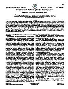
Figure 2: Histogram of running times of all W HT (216 ) binary split trees with no leaves of size 21 . The four types of discrete cosine transforms (DCTs) [Rao and Yip, 1990] are considerably different from the WHT. The following differences are of importance: • While we have used just one basic break down rule for the WHT, there are several very different break down rules for most of the different types of DCTs.

W HT (25 ) =

2

100

where Ik is the k × k identity matrix. This break down rule can then be recursively applied to each of these new smaller WHTs. Thus, W HT (2n ) can be rewritten as any of a large number of different but mathematically equivalent formulas. Any of these formulas for W HT (2n ) can be uniquely represented by a tree, which we call a “split tree.” For example, suppose W HT (25 ) was factored as: [W HT (23 ) ⊗ I22 ][I23 ⊗ W HT (22 )]

1

350

i=1

=

2

400

Number of formulas

1

In general, each node of a split tree should contain not only the size of the transform, but also the transform at that node and the break down rule being applied. A break down rule specifies how a transform can be computed from smaller or different transforms. In Figure 1, the representation was simplified since it only used one break down rule which only involved WHTs. There is a very large number of possible split trees, or equivalently formulas, for a WHT √ of any given size. WHT(2n ) has on the order of Θ((4 + 8)n /n3/2 ) different possible split trees. For example, W HT (28 ) has 16,768 different split trees. Considering only binary WHT split trees slightly reduces the search space, but there are still Θ(5n /n3/2 ) split trees [Johnson and Püschel, 2000]. For the results with the WHT, we used a WHT package, [Johnson and Püschel, 2000], which can implement in code, run, and time WHT formulas passed to it. The WHT package allows leaves of the split trees to be sizes 21 to 28 which are implemented as unrolled straight-line code. This introduces a trade-off since straight-line code has the advantage that it does not have loop or recursion overhead but the disadvantage that very large code blocks will overfill the instruction cache. Figure 2 shows a histogram of the running times of all of the binary split trees of W HT (216 ) with no leaves of size 21 . This data was collected on a Pentium III running Linux. The histogram shows a significant spread of running times, almost a factor of 6 from fastest to slowest. Further, it shows that there are relatively few formulas that are amongst the fastest.

and ⊗ is the tensor or Kronecker product [Beauchamp, 1984]. If A is a m × m matrix and B a n × n matrix, then A ⊗ B is the block matrix product   a1,1 B · · · a1,m B   .. .. ..  . . . . am,1 B · · · am,m B

1

5

Figure 1: Two different split trees for W HT (25 ).

The Walsh-Hadamard Transform of a signal x of size 2n is the product W HT (2n ) · x where n O 1 1 W HT (2n ) = , 1 −1

2

(a)

Signal Processing Background

2

[I23 ⊗ {(W HT (21 ) ⊗ I21 )(I21 ⊗ W HT (21 ))}] 2

• While the break down rule for the WHT allowed for many possible sets of children, most of the break down rules for the DCTs specify exactly one set of children.

As another generalization, k-best dynamic programming keeps track of the k best formulas for each transform and size [Haentjens, 2000; Sepiashvili, 2000]. This softens the dynamic programming assumption, allowing for the fact that a sub-optimal formula for a given transform and size might be the optimal way to split such a node in a larger tree. Unfortunately, moving from standard 1-best to just 2-best more than doubles the number of formulas to be timed. While dynamic programming has been frequently used, it is not known how far from optimal it is at larger sizes where it can not be compared against exhaustive search. Other search techniques with different biases will explore different portions of the search space. This exploration may find faster formulas than dynamic programming finds or provide evidence that the dynamic programming assumption holds in practice. A very different search technique is to generate a fixed number of random formulas and time each. This approach assumes that while the running times of different formulas may vary considerably, there is still a sufficiently large number of formulas that have running times close to the optimal. Evolutionary techniques provide a refinement to the previous approach [Goldberg, 1989]. Evolutionary algorithms add a bias to random search directing it toward better formulas.

• While the WHT factored into smaller WHTs, the break down rules for the DCTs often factor one transform into two transforms of different types or even translate one DCT into another DCT or into a discrete sine transform. Thus, a split tree for a DCT labels the nodes not only with the size of the transform, but also with the transform and the applied break down rule. • The number of factorizations for the DCTs grows even quicker than that for the WHT. For example, DCT type IV already has about 1.9 × 109 different factorizations at size 25 and about 7.3 × 1018 factorizations at size 26 with our current set of break down rules.

3

Search Techniques

There are several approaches for searching for fast implementations of signal processing algorithms, including exhaustive search, dynamic programming, random search, and evolutionary algorithms. One simple approach to optimization is to exhaust over all possible formulas of a signal transform and to time each one on each different machine that we are interested in. There are three problems with this approach: (1) each formula may take a non-trivial amount of time to run, (2) there is a very large number of formulas that need to be run, and (3) just enumerating all of the possible formulas may be impossible. These problems make the approach intractable for transforms of even small sizes. With the WHT, there are several ways to limit the search space. One such limitation is to exhaust just over the binary split trees, although there still are many binary split trees. In many cases, the fastest WHT formulas never have leaves of size 21 . By searching just over split trees with no leaves of size 21 , the total number of trees that need to be timed can be greatly reduced, but still becomes intractable at larger sizes. A common approach for searching the very large space of possible implementations of signal transforms has been to use dynamic programming [Johnson and Burrus, 1983; Frigo and Johnson, 1998; Haentjens, 2000; Sepiashvili, 2000]. This approach maintains a list of the fastest formulas it has found for each transform and size. When trying to find the fastest formula for a particular transform and size, it considers all possible splits of the root node. For each child of the root node, dynamic programming substitutes the best split tree found for that transform and size. Thus, dynamic programming makes the following assumption:

4

STEER for the WHT

We developed an evolutionary algorithm named STEER (Split Tree Evolution for Efficient Runtimes) to search for optimal signal transform formulas. Our first implementation of STEER explicitly only searched for optimal WHT formulas. This section describes STEER for the WHT, while Section 6 describes our more recent implementation of STEER that will work for a variety of transforms. Given a particular size, STEER generates a set of random WHT formulas of that size and times them. It then proceeds through evolutionary techniques to generate new formulas and to time them, searching for the fastest formula. STEER is very similar to a standard genetic algorithm [Goldberg, 1989] except that STEER uses split trees instead of a bit vector as its representation. At a high level, STEER proceeds as follows: 1. Randomly generate a population P of legal split trees of a given size. 2. For each split tree in P , obtain its running time. 3. Let Pf astest be the set of the b fastest trees in P . 4. Randomly select from P , favoring faster trees, to generate a new population Pnew . 5. Cross-over c random pairs of trees in Pnew . 6. Mutate m random trees in Pnew . 7. Let P ← Pf astest ∪ Pnew . 8. Repeat step 2 and following. All selections are performed with replacement so that Pnew may contain many copies of the same tree. Since obtaining a running time is expensive, running times are cached and only new split trees in P at step 2 are actually run.

Dynamic Programming Assumption: The fastest split tree for a particular transform and size is also the best way to split a node of that transform and size in a larger tree. While dynamic programming times relatively few formulas for many transforms, it would need to time an intractable number of formulas for large WHTs. However, by restricting to just binary WHT split trees, dynamic programming becomes very efficient. Between the two extremes, k-way dynamic programming considers split trees with at most k children at any node. Unfortunately, increasing k can significantly increase the number of formulas to be timed.

4.1

Tree Generation and Selection

Random tree generation produces the initial population of legal split trees from which STEER searches. To generate a random split tree, STEER creates a set of random leaves and then combines these randomly to generate a full tree. 3

20

To generate the new population Pnew , trees are randomly selected from P using fitness proportional reproduction which favors faster trees. Specifically, STEER selects from P by randomly choosing any particular tree with probability proportional to one divided by the tree’s running time. This method weights trees with faster running times more heavily, but allows slower trees to be selected on occasion.

4.2

2

5 6 3 2333

14 4

(a)

6

3 7 4 2 4 22

(b)

(c)

Grow

18

5 6 23

3

4

Truncate

13 6 3 4 33

20

18 11

3

4

2

18 11 3

2 36 33

2

7

5 6 3 4 2 33 3

4

2333

Down

20 11

Join

Split

Figure 4: Examples of each kind of mutation, all performed on the tree labeled “Original.”

4.4

Running STEER

Figure 5 shows a typical plot of the running time of the best formula (solid line) and the average running time of the population (dotted line) as the population evolves. This particular plot is for W HT (222 ) on a Pentium III. The average running time of the first generation that contains random formulas is more than twice the running time of the best formula at the end, verifying the wide spread of run times of different formulas. Further, both the average and best run times decrease significantly over time, indicating that the evolutionary operators are finding better formulas.

20

4 14

6

2.2e+09

3 7 4 3 3

(d)

Figure 3: Crossover of trees (a) and (b) at the node of size 6 produces trees (c) and (d) by exchanging subtrees.

4.3

5 23

Up

18

5 6 3 2324 22

2

5 6 3 4 2333 22

Flip 2

Formula running time in CPU cycles

18

20 18

20

20 2

2

6 3 5 33 23

4

20

In a population of legal split trees, many of the trees may have well optimized subtrees, even while the entire split tree is not optimal. Crossover provides a method for exchanging subtrees between two split trees, allowing for one split tree to potentially take advantage of a better subtree found in another split tree [Goldberg, 1989]. Crossover on a pair of trees t1 and t2 proceeds as follows: 1. Let s be a random node size contained in both trees. 2. If no s exists, then the pair can not be crossed-over. 3. Select a random node n1 in t1 of size s. 4. Select a random node n2 in t2 of size s. 5. Swap the subtrees rooted at n1 and n2 . For example, a crossover on trees (a) and (b) at the node of size 6 in Figure 3 produces the trees (c) and (d). 2

4

20 18

Original

2

20

2

5 6 3 2333

Crossover

20

20 18

Mutation

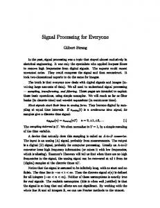
Mutations are changes to the split tree that introduce new diversity to the population. If a given split tree performs well then a slight modification of the split tree may perform even better. Mutations provide a way to search the space of similar split trees [Goldberg, 1989]. We present the mutations that STEER uses with the WHT. Except for the first mutation, all of them come in pairs with one essentially doing the inverse operation of the other. Figure 4 shows one example of each mutation performed on the split tree labeled “Original.” The mutations are: • Flip: Swap two children of a node. • Grow: Add a subtree under a leaf, giving it children. • Truncate: Remove a subtree under a node that could be a leaf, making the node a leaf. • Up: Move a node up one level in depth, causing the node’s grandparent to become its parent. • Down: Move a node down one level in depth, causing the node’s sibling to become its parent. • Join: Join two siblings into one node which has as children all of the children of the two siblings. • Split: Break a node into two siblings, dividing the children between the two new siblings.

average best

2e+09 1.8e+09 1.6e+09 1.4e+09 1.2e+09 1e+09 8e+08 0

20

40

60 80 100 Generations

120

140

Figure 5: Typical plot of the best and average running time of formulas as STEER evolves the population.

5

Search Algorithm Comparison for WHT

Figure 6 shows two different runs of binary dynamic programming on the same machine, namely a Pentium III 450 MHz running Linux 2.2.5-15. For sizes larger than 210 , many of the formulas found in the second run are more than 5% slower than those found in the first run. An analysis of this and several other runs on this same machine shows that the major difference is what split tree is chosen for size 24 . The two fastest split trees for that size have close running times. Since the timer is not perfectly accurate, it times one split tree sometimes faster and sometimes slower than the other from run to run. However, one particular split tree is consistently faster than the other when used in larger sizes. While this specific result is particular to the machine we were using, it demonstrates a general problem with dynamic programming. There may be several formulas for small sizes that all run about equally fast. However, one formula may run 4

100000 Binary 1-Best DP Binary 2-Best DP 3-Way 1-Best DP STEER 5000 Random Formulas Binary NoLeaf1 Exhaustive

Run 1 Run 2

1.15 10000

1.1 Number of Formulas Timed

Running Times Divided by Run 1 Times

1.2

1.05 1 0.95

1000

100

0.9 5

10

15 Log of Size

20

25

10

Figure 6: Two runs of dynamic programming. 1 5

considerably faster as part of a larger split tree than the others. So, if dynamic programming happens to choose poorly for smaller sizes early in its search, then it can produce significantly worse results at larger size than it would if it had choose the right formulas for smaller sizes. Figure 7 compares the best running times found by a variety of search techniques on the same Pentium III. In this particular run, plain binary dynamic programming chose the better formula for size 24 and performs well. All of the search techniques perform about equally well except for the random formula generation method which tends to perform significantly worse for sizes larger than 215 , indicating that some form of intelligent search is needed in this domain and that blind sampling is not effective.

6

Running Times Divided by Binary 1-Best DP Times

1.2

1.15

1.1

1.05

1

0.95

0.9

0.85 10

15 Log of Size

20

20

25

Optimization for Arbitrary Transforms

As part of the SPIRAL research group [Moura et al., 1998], we are developing a system for implementing and optimizing a wide variety of signal transforms, including user-specified transforms. This system begins with a database of signal transforms and break down rules for factoring those transforms that can be extended by users. Mathematical formulas can be generated for fully factored transforms [Püschel et al., 2001], and these formulas can be compiled into executable code [Xiong et al., 2001]. This section discusses how we have adapted search methods to this system so that they can be used to optimize arbitrary transforms, and then empirically compares the search methods. Exhaustive search requires generating every possible formula for a given transform. In the SPIRAL system, this is done by using every applicable break down rule on the transform and then recursively every combination of applicable break down rules on the resulting children. We have also adapted dynamic programming to this new setting. Given a transform to optimize, dynamic programming uses every applicable break down rule to generate a list of possible sets of children. For each of these children, it then recursively calls dynamic programming to find the best split tree(s) for the children, memoizing the results. Each of these possible sets of children are used to form an entire split tree of the original transform. These new split trees are then timed to determine the fastest. STEER as described above used many operators that heavily relied on properties of the WHT. We have adapted STEER to the SPIRAL system so it can optimize arbitrary signal transforms. The following changes were made:

Binary 1-Best DP Binary 2-Best DP 3-Way 1-Best DP STEER 5000 Random Formulas Binary NoLeaf1 Exhaustive

5

15 Log of Size

Figure 8: Number of WHT formulas timed.

1.3

1.25

10

25

Figure 7: Comparison of best WHT running times. Figure 8 compares the number of formulas timed by each of the search methods. A logarithm scale is used along the yaxis representing the number of formulas timed. Effectively all of the time a search algorithm requires is spent in running formulas. The random formula generation method sometimes times less formulas than were generated if the same formula was generated twice. The number of formulas timed by the exhaustive search method grows much faster than all of the other techniques, indicating why it quickly becomes intractable for larger sizes. Clearly plain binary dynamic programming has the advantage that it times the fewest formulas. Of the search methods compared, dynamic programming both finds fast WHT formulas and times relatively few formulas. However, we have also shown that dynamic programming can perform poorly if it chooses a poor formula for one of the smaller sizes. STEER also finds fast formulas but is not as strongly impacted by poor initial choices.

• Random Tree Generation. A new method for generating a random split tree was developed. For a given transform, a random applicable break down rule is chosen, and then a random set of children are generated using the break down rule. This is then repeated recursively for each of the transforms of the children. • Crossover. Crossover remains the same except the definition of equivalent nodes. Now instead of looking for split tree nodes of the same size, crossover must find nodes with the same transform and size. • Mutation. We developed a new set of mutations since the previous ones were specific to the WHT. We have developed three mutations that work in this general setting 5

4 DCT IV 2 RuleDCT4_3


3 DCT II 2 RuleDCT2_2

2 DCT II 2 RuleDCT2_2 DCT II 2

3 DST II 2 RuleDST2_3


DCT IV 2

DST IV 2

2 DST IV 2 RuleDST4_1

DST II 2

DCT II 2

DST II 2

DCT II 2

DCT IV 2

DST IV 2

DST II 2





DCT II 2

Regrow




DCT II 2


Original


DCT IV 2

DST IV 2



DST II 2




2 DCT IV 2 RuleDCT4_3 DCT II 2



DST II 2

DCT II 2




DST II 2 DCT II 2

DST IV 2


DST II 2

DCT II 2



DCT IV 2

DCT II 2


DST II 2

DST II 2

2 DCT IV 2 RuleDCT4_4 DST IV 2

Copy

DCT IV 2

2 DST II 2 RuleDST2_3 DST IV 2

DST II 2

DST II 2

Swap

Figure 9: Examples of each general mutation, all performed on the tree labeled “Original.” Areas of interest are circled. without specific knowledge of the transforms or break down rules being considered. They are:

Formula runtime in nanoseconds

– Regrow: Remove the subtree under a node and grow a new random subtree. – Copy: Find two nodes within the split tree that represent the same transform and size. Copy the subtree underneath one node to the subtree of the other. – Swap: Find two nodes within the split tree that represent the same transform and size. Swap the subtrees underneath the two nodes.


1500

1000

500

For DCT type IV size 24 , exhaustive search was also performed over the space of 31,242 different formulas that can be generated with our current set of break down rules. Figure 12(a) shows the running times of the fastest formulas found by each search algorithm. Figure 12(b) shows the number of formulas timed by each of the search algorithms. The formulas found by the exhaustive search and by STEER are about equally fast while the one found by dynamic programming is slower. However, dynamic programming times very few formulas, and STEER times orders of magnitude less than the exhaustive search.

7

2000

Related Work

A few other researchers have addressed similar goals. FFTW [Frigo and Johnson, 1998] is an adaptive package that produces efficient FFT implementations across a variety of machines. FFTW uses binary dynamic programming to search for an optimal FFT implementation. Outside the signal processing field, several researchers have addressed the problem of selecting the optimal algorithm. Most of these approaches only search among a few

1500

1000

500

0

Size 16

2000

Figure 11: Best DCT size 25 times across 4 types.

Legend DP 1-Best DP 2-Best DP 4-Best STEER

Size 8

2500

Type I Type II Type III Type IV

We ran dynamic programming and STEER on the same Pentium III to find fast implementations of DCTs. Figure 10 shows the running times of the best formulas found by each algorithm for DCT IV across three sizes. Figure 11 shows the same but for the four types of DCTs all of size 25 . Both diagrams indicate that STEER consistently finds the fastest formulas.

2500

3000

0

Figure 9 shows an example of each of these mutations. These mutations are general and will work with arbitrary user specified transforms and break down rules.

3000

Legend DP 1-Best DP 2-Best DP 4-Best STEER

3500

Size 32

Figure 10: Best DCT type IV times across several sizes.

6

inferred. The first author, Bryan Singer, was partly supported by a National Science Foundation Graduate Fellowship.

31242

Number of formulas timed


35000

1000

800

600

400

200

30000

25000

References

20000

[Auslander et al., 1996] L. Auslander, J. Johnson, and R. Johnson. Automatic implementation of FFT algorithms. Technical Report 96-01, Drexel University, 1996. [Beauchamp, 1984] K. Beauchamp. Applications of Walsh and Related Functions. Academic Press, 1984. [Bilmes et al., 1997] J. Bilmes, K. Asanović, C. Chin, and J. Demmel. Optimizing matrix multiply using PHiPAC: a Portable, High-Performance, ANSI C coding methodology. In Proceedings of International Conference on Supercomputing, 1997. [Brewer, 1995] E. Brewer. High-level optimization via automated statistical modeling. In Proceedings of the 5th ACM SIGPLAN Symposium on Principles and Practice of Parallel Programming, 1995. [Frigo and Johnson, 1998] M. Frigo and S. Johnson. FFTW: An adaptive software architecture for the FFT. In Proceedings of International Conference on Acoustics, Speech, and Signal Processing, volume 3, 1998. [Goldberg, 1989] D. Goldberg. Genetic Algorithms in Search, Optimization, and Machine Learning. AddisonWesley, Reading, MA, 1989. [Haentjens, 2000] G. Haentjens. An investigation of CooleyTukey decompositions for the FFT. Master’s thesis, ECE Dept., Carnegie Mellon University, 2000. [Johnson and Burrus, 1983] H. Johnson and C. Burrus. The design of optimal DFT algorithms using dynamic programming. In IEEE Transactions on Acoustics, Speech, and Signal Processing, volume 31, 1983. [Johnson and Püschel, 2000] J. Johnson and M. Püschel. In search of the optimal Walsh-Hadamard transform. In Proceedings of International Conference on Acoustics, Speech, and Signal Processing, 2000. [Lagoudakis and Littman, 2000] M. Lagoudakis and M. Littman. Algorithm selection using reinforcement learning. In Proceedings of International Conference on Machine Learning, 2000. [Moura et al., 1998] J. Moura, J. Johnson, R. Johnson, D. Padua, V. Prasanna, and M. Veloso. SPIRAL: Portable Library of Optimized Signal Processing Algorithms, 1998. http://www.ece.cmu.edu/∼spiral/. [Püschel et al., 2001] Markus Püschel, Bryan Singer, Manuela Veloso, and J. Moura. Fast automatic generation of DSP algorithms. In Proceedings of the International Conference on Computational Science, Lecture Notes in Computer Science 2073, pages 97–106. Springer-Verlag, 2001. [Rao and Yip, 1990] K. Rao and P. Yip. Discrete Cosine Transform. Academic Press, Boston, 1990. [Sepiashvili, 2000] D. Sepiashvili. Performance models and search methods for optimal FFT implementations. Master’s thesis, ECE Dept., Carnegie Mellon University, 2000. [Whaley and Dongarra, 1998] R. Whaley and J. Dongarra. Automatically tuned linear algebra software. In Proceedings of the 1998 ACM/IEEE SC98 Conference, 1998.

15000

10000

5000

0

0

DP 1-Best STEER Exhaustive

54

423

DP 1-Best STEER Exhaustive

(a) (b) 4 Figure 12: DCT type IV size 2 search comparison. algorithms instead of the space of thousands of different implementations we consider in our work. PHiPAC [Bilmes et al., 1997] and ATLAS [Whaley and Dongarra, 1998] use a set of parameterized linear algebra algorithms. For each algorithm, a pre-specified search is made over the possible parameter values to find the optimal implementation. Brewer [1995] uses linear regression to learn to predict running times for four different implementations across different input sizes, allowing him to quickly predict which of the four implementations should run fastest given a new input size. Lagoudakis and Littman [2000] use reinforcement learning to learn to select between two algorithms during successive recursive calls when solving sorting or order statistic selection problems.

8

Conclusion

We have introduced a stochastic evolutionary search approach, STEER, for finding fast signal transform implementations. This domain is particularly difficult in that there is a very large number of formulas that implement the same transform and there is a wide variance in run times between formulas. We have described the development of STEER both specifically for the WHT and for a wide variety of transforms. This later form of STEER is able to optimize arbitrary transforms, even user-defined transforms that it has never before seen. We have shown that STEER finds faster DCT formulas than dynamic programming while still timing significantly less formulas than exhaustive search. In at least one case, STEER was able to find a DCT formula that runs about equally as fast as the optimal one found by exhaustive search. We have shown that a poor early choice can cause dynamic programming to perform sub-optimally. However, STEER has, for the first time, provided evidence that dynamic programming does perform well when searching for fast WHT formulas, if dynamic programming does not make a poor early choice. STEER mainly relies on a tree representation of formulas combined with a set of operators to effectively and legally transform the trees. STEER is thus applicable to general algorithm optimization with similar tree representations.

Acknowledgements We would especially like to thank Jeremy Johnson, José Moura, and Markus Püschel for their many helpful discussions. This research was sponsored by the DARPA Grant No. DABT63-98-1-0004. The content of the information in this publication does not necessarily reflect the position or the policy of the Defense Advanced Research Projects Agency or the US Government, and no official endorsement should be 7

[Xiong et al., 2001] J. Xiong, D. Padua, and J. Johnson. SPL: A language and compiler for DSP algorithms. Proceedings of the ACM SIGPLAN Conference on Programming Language Design and Implementation (PLDI), 2001. To appear.

8