Oikos 124: 949–959, 2015 doi: 10.1111/oik.02385 © 2015 The Authors. Oikos © 2015 Nordic Society Oikos Subject Editor and Editor in-Chief: Christopher Lortie. Accepted 14 February 2015
Woodstoich III Stoichiometric flexibility in response to fertilization along gradients of environmental and organismal nutrient richness Seeta A. Sistla, Alison P. Appling, Aleksandra M. Lewandowska, Benton N. Taylor and Amelia A. Wolf S. A. Sistla (
[email protected]), Dept of Ecology and Evolutionary Biology, Univ. of California, Irvine, 3300 Biological Sciences 3, Irvine, CA 92697, USA. – A. P. Appling (orcid.org/0000-0003-3638-8572), Dept of Natural Resources and the Environment, Univ. of New Hampshire, 181 James Hall, Durham, NH 03824, USA. – A. M. Lewandowska, Inst. for Chemistry and Biology of the Marine Environment, Carl von Ossietzky Univ. Oldenburg, Schleusenstrasse 1, DE-26382 Wilhelmshaven, Germany. – B. N. Taylor, Dept of Ecology, Evolution and Environmental Biology, Columbia Univ., 10th Fl. Schermerhorn Ext., 1200 Amsterdam Ave., New York, NY 10027, USA. – A. A. Wolf, Inst. of the Environment and Sustainability, Univ. of California, Los Angeles, Suite 300, La Kretz Hall, Los Angeles, CA 90095, USA.
Ecosystems globally are undergoing rapid changes in elemental inputs. Because nutrient inputs differently impact high- and low-fertility systems, building a predictive framework for the impacts of anthropogenic and natural changes on ecological stoichiometry requires examining the flexibility in stoichiometric responses across a range of basal nutrient richness. Whether organisms or communities respond to changing conditions with stoichiometric homeostasis or flexibility is strongly regulated by their species-specific capacity for nutrient storage, relative growth rate, physiological plasticity, and the degree of environmental resource availability relative to organismal demand. Using a meta-analysis approach, we tested whether stoichiometric flexibility following nutrient enrichment correlates with the relative fertility of terrestrial and aquatic systems or with the initial stoichiometries of the organism or community. We found that regardless of limitation status, N-fertilization tended to significantly reduce biota C:N and increase N:P, and P fertilization reduced C:P and N:P in both terrestrial and aquatic systems. Further, stoichiometric flexibility in response to fertilization tended to decrease as environmental nutrient richness increased in both terrestrial and aquatic systems. Positive correlations were also detected between the initial biota C:nutrient ratio and stoichiometric flexibility in response to fertilization. Elucidating these relationships between stoichiometric flexibility, basal environmental and biota fertility, and fertilization will increase our understanding of the ecological consequences of ongoing nutrient enrichment across the world.
Ecosystems globally are undergoing unprecedented increases in element inputs. These perturbations can affect ecological stoichiometry – the elemental ratios of organisms in relation to ecosystem structure and function (Sterner and Elser 2002). While the relative availability of elements varies widely in natural environments, biota are characterized by a stricter pattern of element balance (i.e. carbon (C) nitrogen (N) phosphorus (P) trace elements). This pattern reflects the relatively narrow element ratios necessary to catalyze metabolic reactions and build fundamental biological components (e.g. proteins, ATP, nucleic acids) (Elser et al. 2010, Finzi et al. 2011). Metabolic pathways thus couple element cycles from the sub-cellular to global scales. Although biological systems are inherently stoichiometrically constrained, both organisms and ecosystems are (to varying degrees) stoichiometrically flexible. Understanding the extent and controls of stoichiometric flexibility is particularly important because global change factors, such as increasing N and P deposition, can affect ecological stoichiometry and thus the ecosystem functions regulated by these stoichiometric changes (Reich et al. 2006, Finzi et al. 2011,
Sardans et al. 2011, Peñuelas et al. 2013). Therefore, predicting flexibility in organismal and community stoichiometry in a rapidly changing world is of growing concern. Stoichiometric flexibility can be expressed across scales from parts of organisms to entire ecosystems through variation in the elemental balance of individuals and/or the species composition of communities (Sistla and Schimel 2012). At the organismal level, stoichiometric flexibility can occur through changes in nutrient allocation to tissue types or synthesis of subcellular components differing in their characteristic element ratios (Rivas-Ubach et al. 2012). From the community to ecosystem level, stoichiometric shifts can occur through species invasions, altered functional dominance, or changes in the stoichiometries of key species. For example, a fertilization-driven shift in primary producer community structure from herbaceous dominance to shrub dominance would be expected to increase average biomass C:N due to greater wood biomass, an effect that can then feedback to alter soil biogeochemical dynamics (Mack et al. 2004, Sistla et al. 2013). Changes in organismal and ecosystem-level stoichiometries can thus affect a suite of 949
ecosystem processes and functions including food quality, trophic interactions, biogeochemical cycling, and carbon sequestration (Sardans et al. 2012). Sterner and Elser (2002) proposed the concept of stoichiometric homeostasis, termed ‘H’, to represent the degree to which an organism or community maintains its C:N:P ratios when relative element resource availability is perturbed. Whether organisms and ecosystems respond to changing conditions with stoichiometric homeostasis will likely largely depend upon their species-specific capacity for biomass nutrient storage, physiological plasticity, interspecific competitive ability, and the degree of environmental resource availability relative to organismal demand (Elser et al. 2010). While numerous studies have tested the effects of nutrient enrichment on ecosystem functioning, community structure, and organism or community stoichiometry (Rastetter et al. 2001, Sardans et al. 2012, Peñuelas et al. 2013), we have only recently begun to recognize the importance of the variation in stoichiometric flexibility (i.e. change in C:N, C:P, and N:P) over natural fertility gradients (e.g. upwelling zones, arid biomes, highly seasonal systems) and in response to nutrient enrichment (Sardans et al. 2012, Sistla et al. 2014). The stoichiometric response of an organism or community to changes in nutrient availability is central to its performance in an increasingly nutrient-enriched world. Therefore, understanding how stoichiometric flexibility varies in organisms and communities across a wide range of baseline nutrient richness is necessary for a comprehensive understanding of ecological responses to both anthropogenic and natural nutrient pulses. To date, however, there has been no quantitative assessment of how stoichiometric flexibility in response to nutrient enrichment varies with basal nutrient status. We hypothesized that stoichiometric flexibility is regulated by resource limitation, physiological constraints, and growth rate potential (Fig. 1). Nutrient uptake, and therefore plasticity, in response to fertilization should be relatively small when that nutrient is not limiting unless luxury uptake occurs. With the uptake of added nutrients, the extent of stoichiometric flexibility will depend on the growth rate of an organism or community. Organisms in infertile habitats, and those with relatively high C:nutrient biomass ratios, generally display lower maximum potential growth and tissue turnover rates, physiological plasticity and growth response to nutrient addition than do taxa from more fertile soils (Chapin 1980, Crick and Grime 1987, Chapin et al. 1993, Aerts and Chapin 1999, Endara and Coley 2011). For these relatively slow growing organisms or communities, the uptake of a nutrient in response to enrichment should outpace concomitant increases in C biomass, producing a more stoichiometrically plastic response. Thus, C:nutrient stoichiometric flexibility in response to resource enrichment is predicted to negatively correlate with the baseline nutrient richness of an ecosystem and positively correlate with increasing C:nutrient status for organisms and communities (Fig. 1). Using a meta-analysis framework, we tested whether: 1) the C:nutrient stoichiometric flexibility in response to fertilization with a given nutrient negatively correlates with the abundance of that nutrient in the environment or biota (i.e. environmental and biological fertility) and 2) stoichiometric flexibility in response to fertiliza950
Figure 1. Conceptual diagram describing regulation of C:N:P stoichiometric plasticity. Arrows indicate flow of hypotheses and/or causality. Environmental N and P are descriptors of overall system fertility, while initial biomass C:N, C:P and N:P are more biologically-specific indicators of organism nutrient status. Green boxes represent the nutrient manipulations and stoichiometric responses of interest. Blue diamonds and rounded boxes represent decision points relating the nutrient addition to the biological response. Environmental nutrient availability and initial biomass stoichiometry are both interacting controls and indicators of nutrient limitation status and growth rate. When a system is fertilized and organisms are limited by the added nutrient, it is preferentially taken up and the resulting change in biomass N:P is predicted to be high, unless fertilization stimulates uptake of the less limiting nutrient (e.g. N fertilization stimulates P assimilation). Biomass C:P and C:N responses depend further on the growth rate. Nutrient addition more strongly stimulates fast growing organisms (typical of high-nutrient environments and low initial biomass C: N and C:P) than relatively slow growing species, leading to a smaller net change in the biomass C:N or C:P ratios due to greater C acquisition potential.
tion is smaller when the added nutrient is less limiting, as assessed by basal (pre-fertilization) biotic N:P status. Elucidating the relationships between stoichiometric flexibility and ecosystem basal fertility will allow for greater understanding and better predictions of biotic
responses to both natural and anthropogenic nutrient enrichment.
Methods Literature review To identify studies to test our hypotheses, we used ISI Web of Science to search the terms: ‘C:N and fert*’, ‘C:P and fert*’, ‘N:P and fert*’, all combinations of ‘C’, ‘N’, and/ or ‘P’ and ‘fert*’, ‘stoichiometry and fert*’, nutrient and (estuar* or marine or freshwater or aquatic or lake or stream or river) and (fertiliz* or addition or amendment or enrichment) following meta-analysis search criteria adapted from Pullin and Stewart (2006) and Cote et al. (2013). This search yielded 9000 possible hits; we used Google Scholar to check for additional relevant papers. For terrestrial systems, we included studies performed on species and/or communities planted in their native environment, restored prairies, managed forests, and tree plantations (LeBauer and Treseder 2008), but excluded crop systems and greenhouse or laboratory studies, which are characterized by substantial alteration of the natural substrate and/or environmental conditions. For aquatic systems, mesocosm studies conducted in natural field conditions were included, but laboratory studies were excluded. These search criteria were further narrowed by requiring that data were available for each study for: 1) more than one elemental response for C, N, or P (e.g. papers that only reported a change in N, but not C or P, were excluded) and 2) total soil N or P for terrestrial systems (Cleveland and Liptzin 2007), total water column N or P for aquatic systems, total sediment N or P for benthic aquatic systems (Smith 2006), or extractable sediment or water column N or P for aquatic systems (which often did not report total N or P). When necessary, we supplemented the original studies with abiotic data from other publications on the same sites. We restricted our analysis to studies that directly manipulated resource availability (N, P, or N combined with P). Data collection Data were extracted from published studies either from tables or from figures using Data Thief ( www.datathief.org ). We considered studies within independent references that were conducted nearby (e.g. same field station) to be independent (LeBauer and Treseder 2008). If study site coordinates were not directly reported, longitude and latitude were estimated from the provided site information using Google Maps ( www.google.com/maps ). From each study, we recorded the following information: trophic level (primary producer, heterotrophic microbes), functional type (terrestrial: forbs and graminoids, shrubs and trees, soil microbes; aquatic: macrophytes, microphytes including: periphyton, phytoplankton, epilithon, seston), level of biological organization for which stoichiometric response was reported (microscopic community, foliar, litter, stem, root), ecosystem type (terrestrial or aquatic, which included both marine and freshwater studies), habitat (grassland, deciduous forest, evergreen forest, boreal forest,
tropical forest, aquatic, tundra, desert, shrubland (including one heathland study), tropical grassland), limiting resource(s) (binned as: N, P, and ‘other’, which included: co-limitation by N and P, additional resource limitation, and no reported resource limitation), type of fertilization (N, P or N P), amount of fertilization, experimental duration, and environmental nutrient availability (%N and/or %P measured as g nutrient per g dry weight, and/or dissolved N and P). Bulk density and sampling depth were used to convert environmental nutrient data from volume- to mass-based values when necessary. The mean and standard error (sx) or standard deviation (s) of the control and fertilized biomass elemental ratios (C:N, C:P, N:P) were recorded when reported. Otherwise, ambient and fertilized C:N:P ratios of organisms or communities were calculated from reported means and standard errors of C, N and/or P tissue concentrations using standard rules for error propagation through division (Lehrter and Cebrian 2010). Standard deviation was calculated from studies reporting sx (s sx n ). For the studies (two) that did not report sx, s was estimated using the reported significance (P), treatment and control means (Xt and Xc , respectively) and degrees of freedom (df ) using a two-tailed t distribution, where: s ≅ ( XT X C ) t( P 2, df ) This method overestimates variance relative to a direct calculation, thereby conservatively weighting these studies in the meta-analysis (LeBauer and Treseder 2008). For terrestrial systems, unfertilized (ambient condition) total soil N and P were recorded when reported, or were derived from other publications describing the same site. Ambient and fertilized extractable soil nutrients were also recorded when reported. Analogously, total dissolved suspended N and P were recorded for aquatic studies when possible; water-column total nitrogen: total phosphorus (TN: TP) ratio is a key indicator of primary producer nutrient limitation in both marine and freshwater systems (Dodds 2003, Smith 2006). A large proportion of aquatic studies did not report total N or P but did report extractable nutrients; however, dissolved inorganic N and P are not considered robust proxies for either TN and TP (respectively) or system nutrient limitation (Jackson and Williams 1985, Dodds 2003) and were therefore not included in the regression analyses. Because data for different years and/or fertilization levels in a site are not independent of one another, we used the final time period and highest fertilization level for studies that included multiple time points and/ or fertilization levels. Statistical analysis We ultimately included 81 publications (Supplementary material Appendix 1), from which we derived 397 individual studies (unique combinations of site, fertilization treatment and level of biological organization (microphyte or microbial community, foliar, litter, stem or root)). When publications reported observations from multiple sites or under different experimental conditions, they were considered independent studies. For each study, we calculated average biological molar ratios or total element concentrations to estimate 951
stoichiometric response effect sizes using Hedges’ d, which describes the standardized difference in means between the treatment and control (X‒t and X‒c, respectively) (Hedges and Olken 1985): Xt XC Hedges¢ d J (nt 1) st2 (nc 1) sc2 nt nc 2 and J 1
3 4 ( nt nc 2 ) 1
Where st and sc are standard deviations and nt and nc are sample sizes of the treatment and the control, respectively. We calculated the overall effect of each fertilizer type (N, P or N P) on sites within each system type (terrestrial or aquatic) using mixed effect models with a restricted maximum likelihood approach. Level of biological organization was a fixed factor and publication ID was used as a random effect to account for the within-study similarity (i.e. results from the same publication are potentially more closely related than separate publications). The 95% confidence intervals (CI) were used to test if the effect was significantly different from 0. An effect size (d) that is not significantly different from zero indicates no fertilization effect. Values above 0 indicate that the fertilization increased either C:N, C:P or N:P ; values below 0 indicate a decrease in these stoichiometric ratios. The Q statistic was used to test for total heterogeneity of variances in effect sizes across studies (Hedges and Olken 1985). Factorial ANOVA was used to test whether fertilizer effects on biomass C:N, C:P and N:P ratios were different between system types (aquatic and terrestrial) or levels of biological organization (microorganisms versus macroorganisms). The influence of fertilization type, system, and nutrient limitation status on stoichiometric response was also tested using ANOVA. We used regression analyses to relate stoichiometric flexibility to basal environmental nutrient availability (total environmental N and P) and initial biological stoichiometry (C:N, C:P and N:P). We quantified stoichiometric flexibility with a modified natural-log-transformed flexibility index (PIv) (Valladares et al. 2006), where: modified PIV ln
Xt Xc Xc
This modified PIv is an index of the stoichiometric change relative to the original elemental ratio, allowing us to detect patterns in stoichiometric flexibility across systems. Using the absolute value of the difference between Xt and Xc (instead X of ln t ) equally weights increases and decreases in Xc stoichiometric ratios of the treatment relative to control (i.e. a change in C:N from 10 to 8 with fertilization is equally stoichiometrically flexible to a change from 10 to 12), thereby defining a stoichiometric flexibility effect size independent of the direction of change. We explored potential relationships between stoichiometric response to fertilization and basal ecosystem (soil or water) fertility and basal organismal C:N, C:P and N:P. Because environmental nutrient concentrations are often 952
log-normally distributed (Hartman and Richardson 2013), these element pools and ratios were natural-log transformed to improve normality. We ran regressions separately for each explanatory variable (environmental or basal biota nutrient status), fertilizer type applied (N, P or N P), and study system (terrestrial and aquatic). We included level assayed (community, foliar, litter, stem, or root) and limitation status (N, P, other) as fixed factors and publication ID as a random effect. Within aquatic systems, an additional fixed factor was used to distinguish between studies reporting total sediment nutrients and those reporting water column or porewater TN or TP. We extracted p values for the fixed effects using the ‘lmerTest’ package, which estimates degrees of freedom by the Kenward–Roger’s approximation (Kuznetsova et al. 2014). Our focus in this analysis was on the size and significance of the slope coefficients relating flexibility to environmental and biotic nutrient richness. Statistical significance was denoted at p 0.05; marginally significant results (p 0.1) were also reported. All analyses were conducted using R ver. 3.0.3 (). The ‘ggplot2’ package was used to create figures (Wickham 2009) and the ‘metafor’ package was used to complete the meta-analysis (Viechtbauer 2010).
Results Overall fertilization effects on biota stoichiometry Data were synthesized from 397 studies from latitudes ranging from tundra to tropical systems and encompassing tundra, forest, shrubland, grassland, marine and freshwater ecosystems across all levels of biological organization (from leaves and roots to microscopic communities) (Fig. 2, Table 1). Marine and freshwater studies did not significantly differ in their C:N, C:P or N:P response to fertilization and were binned for all analyses (henceforth, aquatic systems). Across all fertilization treatments, resource enrichment decreased biomass C:N and C:P in both terrestrial and aquatic systems, and significantly reduced biomass N:P only in aquatic systems (Fig. 3, Table 2). When grouped by system and fertilization type, N fertilization reduced biomass C:N and increased biomass N:P in both terrestrial and aquatic systems. P fertilization reduced C:P and N:P in both aquatic and terrestrial systems. Fertilization with both N and P (hereafter ‘NP fertilization’) reduced biomass C:N and C:P in aquatic systems, but only significantly decreased biomass C:N in terrestrial systems. A complete summary of the Hedges’ d effect sizes for fertilization of aquatic and terrestrial systems can be found in Table 2. We tested whether the strength of the effects observed in both systems under the same fertilization treatment differed between aquatic and terrestrial systems using an ANOVA. NP fertilization more strongly reduced aquatic biomass C:N than terrestrial C:N (F 8.7, DF 1, p 0.005). No other significant differences between aquatic and terrestrial stoichiometric responses to fertilization were detected. Fertilization similarly influenced aquatic macrophyte and microphyte stoichiometries; however, N fertilization decreased macrophyte biomass C:N (d –1.14, 95%
Figure 2. Map of study site locations with habitat type indicated.
Table 1. Sample sizes of studies reporting C:N, C:P, N:P, C, N or P for categories used in the meta-analysis and regression analyses of modified PIv . Response variable reported* Category System
C:N
C:P
N:P
C
N
P
freshwater marine terrestrial
Variable
No. of studies 62 115 220
45 71 70
24 59 44
38 98 193
11 40 62
43 77 202
21 76 180
aquatic desert deciduous forest evergreen forest grassland shrubland tundra tropical forest tropical grassland
177 6 3 13 48 6 29 100 15
116 0 3 13 19 2 8 25 0
83 0 0 2 16 0 1 25 0
136 6 0 2 44 4 22 100 15
50 0 3 11 19 0 4 25 0
119 6 2 13 35 6 25 100 15
97 6 0 2 31 4 22 100 15
aquatic macrophyte aquatic microphyte mixed forbs/graminoids soil microbes trees/shrubs
112 65 62 9 149
82 34 18 8 44
54 29 15 3 26
83 53 59 3 131
32 19 17 9 36
89 31 49 8 145
62 35 46 3 131
foliar stem root litter community
216 23 36 48 74
102 7 16 19 42
74 0 9 12 32
187 16 29 41 56
52 6 8 19 28
185 22 28 48 39
159 16 23 41 38
nitrogen phosphorus
284 249
139 117
87 86
226 211
86 67
233 191
192 171
nitrogen phosphorus unidentified/co-limited
129 70 198 397
70 34 82 186
36 32 59 127
94 64 171 329
42 14 57 113
109 44 169 322
79 50 148 277
Habitat
Species type
Level assayed
Nutrient added*
Limitation status
Total*
* For these categories an individual study may have reported multiple variables (i.e. many studies added both N and P). Thus, the number of studies in this section does not sum to the total number of individual studies in the dataset (397).
953
Figure 3. Meta-analysis results reporting Hedges’ d effect size for change in C:N, C:P and N:P in response to fertilization (N, P, NP pooled) for terrestrial and aquatic systems. The dashed line represents no effect of fertilization on stoichiometry (zero). Significance is denoted as follows: * p 0.05; ** p 0.01; *** p 0.001. Bars represent 95% confidence intervals.
CI –2.01– –0.27, p 0.01) and increased N:P (d 0.67, 95% CI 0.12–1.21, p 0.02) but did not have a corresponding effect on microphyte stoichiometry. Additionally, although NP fertilization reduced aquatic microphyte biomass N:P (d –0.63, 95% CI –1.19– –0.07, p 0.03) and C:P (d –0.96, 95% CI –1.63– –0.39, p 0.005), it did not significantly affect macrophyte N:P or C:P. Relationships between limitation status and fertilization treatment on biota stoichiometry In N limited systems, N and NP fertilization reduced terrestrial biota C:N, but only NP fertilization reduced aquatic biota C:N. N fertilization also marginally increased N limited aquatic biomass C:P. N and P fertilization, respectively, increased and decreased biomass N:P in both terrestrial and aquatic N-limited systems, but NP fertilization did not affect N limited biomass N:P in either system. No C:P responses to fertilization were recorded in N limited terrestrial systems,
while aquatic biomass C:P declined with NP fertilization. In P limited terrestrial and aquatic systems, N and NP fertilization reduced biomass C:N, while P and NP fertilization reduced biomass C:P. P fertilization reduced biomass N:P in both aquatic and terrestrial P limited systems; however, N enrichment increased biomass N:P and NP enrichment reduced biomass N:P only in P limited aquatic systems (Table 3). Systems that were either co-limited or did not have a specific limitation noted were similarly sensitive to fertilization as N or P limited systems. N and NP enrichment reduced biomass C:N, NP fertilization reduced aquatic (but not terrestrial) biomass C:P, and P fertilization reduced N:P in both terrestrial and aquatic systems. In terrestrial systems, P fertilization also reduced biomass C:P, while N enrichment increased C:P. These effects were not detected in aquatic systems (Table 3). When terrestrial and aquatic systems were considered together, limitation status significantly affected biota C:N, C:P and N:P response to NP
Table 2. Summary of biomass stoichiometric responses to N, P and N P fertilization treatments, separated by system (but aggregated across biological levels and ecosystems). Responses with a sample size (n) of 2 or less were excluded from the analyses. Significant effects (p 0.05) are indicated in bold. Fertilization N N N N N N P P P P P P N and P N and P N and P N and P N and P N and P
954
System
Response
n
Effect size (d)
SE
p
95% CI interval
aquatic aquatic aquatic terrestrial terrestrial terrestrial aquatic aquatic aquatic terrestrial terrestrial terrestrial aquatic aquatic aquatic terrestrial terrestrial terrestrial
biomass C:N biomass C:P biomass N:P biomass C:N biomass C:P biomass N:P biomass C:N biomass C:P biomass N:P biomass C:N biomass C:P biomass N:P biomass C:N biomass C:P biomass N:P biomass C:N biomass C:P biomass N:P
36 26 44 33 15 74 29 23 40 15 14 61 40 26 41 20 13 54
0.83 0.19 0.53 1.28 0.26 0.80 0.04 1.33 1.22 0.25 1.06 1.45 1.40 0.86 0.36 0.95 0.76 0.30
0.36 0.20 0.21 0.29 0.27 0.18 0.16 0.52 0.24 0.16 0.33 0.30 0.28 0.30 0.23 0.25 1.24 0.31
0.02 0.34 0.01 0.0001 0.33 0.0001 0.80 0.001 0.0001 0.11 0.002 0.0001 0.0001 0.004 0.12 0.0002 0.54 0.33
1.54 – 0.13 0.20 – 0.58 0.11 – 0.94 1.85 – 0.71 0.27 – 0.80 0.44 – 1.15 0.36 – 0.28 2.35 – 0.32 1.69 – 0.74 0.56 – 0.06 1.71 – 0.40 2.05 – 0.85 1.95 – 0.86 1.44 – 0.28 0.81 – 0.10 1.44 – 0.45 3.19 – 1.66 0.89 – 0.30
Table 3. Summary of biomass stoichiometric responses to N, P and N P fertilization treatments, separated by system (but aggregated across biological levels and ecosystems) and limitation status (‘other’ includes co-limitation by N and P as well as other resources or unidentified resource limitation). Responses with a sample size (n) of 2 or less were excluded from the analyses. Significant effects (p 0.05) and marginally significant results (p 0.1) are indicated in bold.
Terrestrial systems
Aquatic systems
Limitation
Fertilization
N N N N N N N N N P P P P P P P P P other other other other other other other other other N N N N N N N N N P P P P P P P P P other other other other other other other other other
N P NP N P NP N P NP N P NP N P NP N P NP N P NP N P NP N P NP N P NP N P NP N P NP N P NP N P NP N P NP N P NP N P NP N P NP
Response
n
Effect size (d)
SE
p
95% CI interval
biomass C:N biomass C:N biomass C:N biomass C:P biomass C:P biomass C:P biomass N:P biomass N:P biomass N:P biomass C:N biomass C:N biomass C:N biomass C:P biomass C:P biomass C:P biomass N:P biomass N:P biomass N:P biomass C:N biomass C:N biomass C:N biomass C:P biomass C:P biomass C:P biomass N:P biomass N:P biomass N:P biomass C:N biomass C:N biomass C:N biomass C:P biomass C:P biomass C:P biomass N:P biomass N:P biomass N:P biomass C:N biomass C:N biomass C:N biomass C:P biomass C:P biomass C:P biomass N:P biomass N:P biomass N:P biomass C:N biomass C:N biomass C:N biomass C:P biomass C:P biomass C:P biomass N:P biomass N:P biomass N:P
15
1.73
0.45
0.0001
2.61 – 0.84
3
1.00
0.43
0.02
1.85 – 0.15
17 12 13 6 6 6 6 6 6 11 15 11 12 9 13 8 8 9 46 34 34 11 7 13 7 4 5 14 11 11 13 12 5 12 11 5 17 16 10 12 10 22 7 8 16 13 13 20
1.01 1.01 0.10 0.52 0.12 0.64 0.13 1.80 1.75 0.23 1.71 0.88 0.87 0.30 0.71 0.56 0.68 0.99 0.66 1.34 0.56 1.65 0.07 2.98 0.50 1.03 0.82 0.74 1.17 0.28 1.69 0.20 1.79 0.24 1.81 2.07 0.81 1.79 0.85 0.64 0.15 0.89 0.24 1.32 0.69 0.35 0.82 0.35
0.23 0.50 0.40 0.30 0.30 0.31 0.29 0.36 0.35 0.61 0.63 0.81 0.32 0.19 0.30 0.21 0.20 0.20 0.24 0.47 0.33 1.15 0.26 0.76 0.25 0.70 0.38 0.37 0.30 0.22 0.55 0.33 0.89 0.51 0.70 1.08 0.46 0.47 0.35 0.23 0.25 0.20 0.29 0.97 0.33 0.27 0.43 0.29
0.0001 0.04 0.80 0.08 0.69 0.04 0.65 0.0001 0.0001 0.71 0.01 0.28 0.01 0.11 0.02 0.01 0.001 0.20 0.01 0.004 0.09 0.15 0.80 0.0001 0.06 0.14 0.03 0.05 0.0001 0.21 0.002 0.54 0.04 0.63 0.01 0.06 0.08 0.0001 0.01 0.005 0.56 0.0001 0.42 0.18 0.04 0.20 0.05 0.21
0.56 – 1.47 1.98 – 0.04 0.68 – 0.87 1.11 – 0.07 0.72 – 0.48 1.24 – 0.04 0.71 – 0.44 2.51 – 1.10 2.43 – 1.06 0.97 – 1.42 2.95 – 0.47 2.47 – 0.71 1.50 – 0.23 0.66 – 0.07 1.30 – 0.11 0.16 – 0.96 1.08 – 0.29 2.51 – 0.54 0.19 – 1.13 2.26 – 0.42 1.21 – 0.09 3.90 – 0.60 0.57 – 0.44 4.46 – 1.49 0.02 – 0.95 2.41 – 0.34 1.56 – 0.07 0.01 – 1.48 1.76 – 0.58 0.15 – 0.71 2.77 – 0.60 0.85 – 0.45 3.53 – 0.05 0.76 – 1.25 3.18 – 0.43 4.18 – 0.05 0.09 – 1.71 2.72 – 0.87 1.54 – 0.17 1.09 – 0.19 0.35 – 0.65 1.27 – 0.51 0.34 – 0.81 3.23 – 0.59 1.33 – 0.05 0.18 – 0.88 1.66 – 0.01 0.92 – 0.23
955
fertilization (DF 2, p 0.05 in all cases) and C:N response to N fertilization (DF 2, p 0.04). Relationships between basal environmental nutrient richness and stoichiometric flexibility in response to fertilization In terrestrial and aquatic systems, greater soil and sediment N and P availability was correlated with a decline in organism C:nutrient stoichiometric flexibility in response to fertilization (Table 4). As soil nutrient availability (%N and %P) increased, there was a decline in the modified PIv (flexibility) of terrestrial biomass C:P under P fertilization. No significant relationships were detected between terrestrial C:N stoichiometric flexibility and soil %N or %P; however, N:P flexibility declined with increasing soil N availability in response to N fertilization, and N:P flexibility declined with increasing soil P availability in response to both N and NP fertilization (Table 4). In aquatic systems, organismal C:N and C:P flexibility declined with increasing sediment %N under N fertilization. There were negative correlations between sediment %P and several types of aquatic biomass flexibility, including C:N flexibility in response to N fertilization and C:P flexibility in response to N, P and NP enrichment. Dissolved TP was also negatively correlated with C:P flexibility with NP fertilization (Table 4). Relationships between basal organismal nutrient richness and stoichiometric flexibility in response to fertilization Greater basal (ambient conditions) biomass C:P and C:N (e.g. increasing P and N limitation, respectively) was
positively correlated with greater stoichiometric flexibility in response to fertilization with the reported limiting resource (Table 4, Fig. 4). Both terrestrial and aquatic organism basal C:N were positively correlated with the flexibility of C:N in response to NP fertilization. In terrestrial systems, basal biomass C:P was also positively correlated with the flexibility of C:P in response to P fertilization and C:N flexibility in response to NP fertilization. However, increasing terrestrial basal biomass C:P was negatively correlated with both C:N flexibility and N:P flexibility in response to P and N fertilization, respectively. The relationship between basal biomass N:P and stoichiometric flexibility in response to fertilization was similar between aquatic and terrestrial systems. Basal biomass N:P (i.e. greater biomass N relative to P) was positively correlated with aquatic biomass N:P flexibility in response to P fertilization. In terrestrial systems, increasing basal biomass N:P was positively correlated with C:P flexibility with P fertilization and negatively correlated with C:N flexibility and N:P flexibility in response to P fertilization and N fertilization, respectively (Table 4).
Discussion Our analyses demonstrate that in both terrestrial and aquatic systems, C:nutrient flexibility in response to fertilization generally increases with lower environmental nutrient availability and with greater organismal basal C:nutrient status (i.e. more nutrient-limited biota). These patterns were robust across multiple levels of biological organization. We know of no other quantitative assessment testing the relationships between fertilization and stoichiometric flexibility across biological scales in conjunction with environmental
Table 4. Linear regression results of modified PIv versus environmental N and P, and initial biomass C:N, C:P and N:P. Responses tested were the modified PIv
ln
Xt Xc Xc
of C:N, C:P and N:P of aquatic and terrestrial systems. Values include the sign and magnitude of the
regression slope, p-value of the linear model, and number of studies used in the model in the form: /– slope (p-value, sample size). Brackets indicate significant regression results for aquatic (non-sediment) total N and P. Marginally significant results (p 0.1) are reported; significant results (p 0.05) are indicated in bold. Plots of all regressions can be found in Supplementary material Appendix 2. System
Response Fertilizer
Aquatic
C:N
C:P
N:P
Terrestrial C:N
C:P
N:P
956
N P NP N P NP N P NP N P NP N P NP N P NP
Soil or sediment %N (aquatic TN) 1.2 (0.007, 11)
Soil or sediment %P (aquatic TP)
Ambient biomass C:N
Ambient biomass C:P
Ambient biomass N:P
1.3 (0.006, 8) 0.87 (0.02, 48)
0.98 (0.01, 10)
1.1 (0.007, 8) 2.7 (0.09, 10) 1.3 (0.01, 10) [0.45 (0.05, 10)]
0.48 (0.05, 31) 3 (0.001, 26) 0.23 (0.06, 41)
1.2 (0.1, 14) 1 (.0.1, 15)
1.5 (0.01, 14)
0.54 (0.008, 14)
1.4 (0.002, 14)
1.7 (0.004, 14)
0.33 (0.02, 63)
1.1 (0.9, 15)
1.7 (0.007, 22) 1.3 (0.02, 14) 0.53 ( 0.0001, 69)
0.37 (0.02, 48)
0.89 (0.01,74)
Figure 4. Examples of regression models relating stoichiometric flexibility/plasticity (modified PIv) to biological nutrient richness in terrestrial systems with P fertilization (left panel) and aquatic systems with NP fertilization (right panel). The y axis represents the response size of biomass C:P when fertilized, relative to basal biomass C:P for terrestrial (p-value of the linear model 0.002) and aquatic (p 0.05) systems.
and biological fertility gradients. Combined with the more commonly tested direct effects of fertilization on biomass C:N:P ratios (Elser et al. 2007, Sardans et al. 2011), identifying these patterns of stoichiometric flexibility across biological and environmental fertility gradients strengthens our understanding of the ability for organisms and ecosystems to respond to nutrient enrichment globally. Across systems and N and P fertilization regimes, biotic C:N and C:P declined with nutrient enrichment, while biomass N:P was significantly reduced only in aquatic systems. Fertilization with a limiting resource under single resource limitation conditions is expected to increase the C:nutrient status of non-limiting resources (Bracken et al. 2015) by stimulating growth and C uptake more than uptake of other nutrients. Only in N-limited aquatic systems did fertilization with the limiting resource (N) dilute the non-limiting nutrient (P), thereby increasing biomass C:P. In terrestrial systems, N fertilization increased biomass C:P under ‘other’ limiting conditions, which included systems identified as co-limited by N and P, as well as without an identified resource limitation. Because P fertilization did not analogously increase C:N in any P-limited system, these results suggest that organisms identified by researchers as P-limited are likely co-limited by another resource or resources. Uncertainty in defining nutrient limitation status complicates projecting the effects of nutrient enrichment on ecological function (Güsewell 2004, Mayor et al. 2014); we propose that studying patterns of stoichiometric responses to fertilization across environmental and biological fertility gradients can serve as a complementary method to predict the consequences of nutrient enrichment on organisms and ecosystems. We hypothesized that as environmental or biological fertility declines for a given nutrient, the C:nutrient stoichiometric flexibility in response to fertilization with that nutrient will increase. This pattern was detected in both terrestrial and aquatic systems. For example, as ambient terrestrial biomass C:P increased (i.e. as P became more limiting), C:P flexibility with P fertilization increased, and as soil %P increased (i.e. as P became less limiting), C:P flexibility with P fertilization declined. Analogously, aquatic
sediment nutrients and TP were also negatively correlated with biomass C:P flexibility in response to P and NP fertilization, and aquatic biota C:N flexibility in response to N fertilization declined with increasing sediment %N. Reduced stoichiometric flexibility with greater nutrient availability – as inferred by either basal environmental or biotic nutrient status – reflects two distinct but potentially complementary mechanisms. More nutrient-rich systems may be less likely to take up additional N or P than more limited systems. Alternatively, the ability of organisms to relatively rapidly increase C acquisition in response to nutrient enrichment is likely greater in more fertile systems (Chapin et al. 1986). Thus, if nutrient uptake is not accompanied by an increase in growth (i.e. luxury uptake), C:nutrient ratios in these systems will at least transiently decrease, driving high stoichiometric plasticity. Our study indicates support for both mechanisms. Regardless of limitation status or system, N fertilization tended to significantly reduce biota C:N and increase N:P, and P fertilization reduced C:P and N:P. This pattern suggests that some amount of luxury consumption – the process by which biota take up a nutrient in the absence of limitation by that nutrient – is widespread. Stoichiometric plasticity in response to fertilization was also predicted to be relatively small when the added nutrient is not limiting. Along a gradient of increasing basal biomass N:P ratios (i.e. increasing P limitation relative to N limitation), this hypothesis was supported in both aquatic and terrestrial habitats. As basal biomass N:P increased, terrestrial C:P and aquatic N:P stoichiometric flexibility increased in response to P fertilization, and terrestrial biota N:P flexibility declined in response to N fertilization. Similarly, as soil %N and %P increased, N:P flexibility declined in response to N and NP fertilization, while increasing aquatic biomass C:N (i.e. increasing N limitation) was positively correlated with N:P flexibility under N fertilization. Intriguingly, greater sediment %N was negatively correlated with aquatic biota C:P plasticity in response to N fertilization. This result complements the observation that N fertilization increased aquatic biomass C:P under conditions of N limitation, but otherwise did not significantly 957
affect biomass C:P. Therefore, as environmental N availability increases (i.e. becomes less limiting), the impact of N fertilization on aquatic biota C:P should, and did, decline. Similarly, aquatic biota C:N and C:P flexibility in response to N fertilization declined with greater sediment %P. These relationships indicate that increased environmental P availability mitigates the N fertilization-driven dilution effect on biomass C:P by increasing the potential for P uptake, while reducing the decline in biomass C:N by increasing C acquisition potential. Supporting this hypothesis, the greatest reduction of aquatic biomass C:N with N fertilization occurred under conditions of P limitation. In terrestrial systems, increasing basal biomass C:P and N:P (i.e. increasing P limitation) was negatively correlated with C:N flexibility in response to P fertilization. Terrestrial biota C:N tended to decline with P fertilization, suggesting that greater P availability can stimulate N acquisition (Treseder and Vitousek 2001); our regression results suggest that this effect is governed by biotic P status. It remains an open question whether the patterns of stoichiometric flexibility observed here would be seen across spatial and temporal scales. Short-term stoichiometric responses to nutrient inputs occur at the scale of an individual – that is, changes in the C:N:P ratios and stoichiometric flexibility are due to the capacity of an individual organism to respond to nutrient addition. However, longer-term responses to fertilization may also alter community composition (Mack et al. 2004, Allison et al. 2007), thereby shifting community-level stoichiometries. Further, nutrient enrichment may preferentially stimulate C loss from nutrient poor systems if it accelerates decomposition by increasing litter or detrital nutrient richness (Allison and Vitousek 2004). Thus, long-term differences in stoichiometric flexibility – and its biogeochemical consequences – may be due to individual- or species-level shifts in C and nutrient acquisition and storage, or due to shifts in communities and the average C:N:P ratios of new community members. To understand how changes in ecosystem fertility impact biogeochemical cycling, studies are needed that integrate long-term fertilization effects scaling from individuals to communities. Our analysis demonstrates clear relationships between fertility gradients and stoichiometric flexibility in the face of increasing nutrient availability across broad biological scales. Identifying whether ecosystem nutrient richness is correlated with stoichiometric flexibility in response to nutrient enrichment strengthens our ability to project the impact of anthropogenic activities on ecosystem biogeochemical dynamics. Increasing nutrient availability in terrestrial and aquatic systems due to atmospheric N deposition, fertilizer application, natural stochastic processes such as upwelling, and shifts in decomposition dynamics with climate warming (among other factors) can profoundly affect ecosystem functions and ecological relationships (Matson et al. 1999, Rustad et al. 2001, Bennett et al. 2001, Finzi et al. 2011). Although many studies have examined the role of fertilization in altering environmental and biological stoichiometric relationships, our findings are the first to demonstrate that these processes may lead to predictable shifts in C:N:P stoichiometries across a range of fertility gradients and biological scales. 958
Acknowledgements – This paper was produced as part of the Woodstoich III workshop on ecological stoichiometry. Many thanks to the Woodstoich conference participants for helpful comments and discussion. We also thank Steve Allison for greatly strengthening this manuscript. Financial support was provided by the Charles Perkins Center at the University of Sydney and the U.S. National Science Foundation (award DEB-1347502). SS was supported by the NOAA Climate and Global Change Postdoctoral Fellowship Program, administered by the University Corporation for Atmospheric Research.
References Aerts, R. and Chapin III, F. S. 1999. The mineral nutrition of wild plants revisited: a re-evaluation of processes and patterns. – Adv. Ecol. Res. 30: 1–67. Allison, S. D. and Vitousek, P. M. 2004. Rapid nutrient cycling in leaf litter from invasive plants in Hawai’i. – Oecologia 141: 612–619. Allison, S. D. et al. 2007. Nitrogen fertilization reduces diversity and alters community structure of active fungi in boreal ecosystems. – Soil Biol. Biochem. 39: 1878–1887. Bennett, E. M. et al. 2001. Human impact on erodable phosphorus and eutrophication: a global perspective. – Bioscience 51: 227–234. Bracken, M. E. S. et al. 2015. Signatures of nutrient limitation and co-limitation: responses of autotroph internal nutrient concentrations to nitrogen and phosphorus additions. – Oikos 124: 113–121. Chapin III, F. S. 1980. The mineral nutrition of wild plants. – Annu. Rev. Ecol. Syst. 11: 233–260. Chapin III, F. S. et al. 1986. The nature of nutrient limitation in plant communities. – Am. Nat. 127: 48–58. Chapin III, F. S. et al. 1993. Evolution of suites of traits in response to environmental stress. – Am. Nat. 142: S78–S92. Cleveland, C. C. and Liptzin, D. 2007. C:N:P stoichiometry in soil: is there a “Redfield ratio” for the microbial biomass? – Biogeochemistry 85: 235–252. Cote, I. et al. 2013. Gathering data: search literature and selection criteria. – In: Koricheva, J. et al. (eds), Handbook of metaanalysis in ecology and evolution. Princeton Univ. Press, pp. 37–51. Crick, J. C. and Grime, J. P. 1987. Morphological plasticity and mineral nutrient capture in two herbaceous species of contrasted ecology. – New Phytol. 107: 403–414. Dodds, W. 2003. Misuse of inorganic N and soluble reactive P concentrations to indicate nutrient status of surface waters. – J. N. Am. Benthol. Soc. 22: 171–181. Elser, J. J. et al. 2007. Global analysis of nitrogen and phosphorus limitation of primary producers in freshwater, marine and terrestrial ecosystems. – Ecol. Lett. 10: 1135–1142. Elser, J. J. et al. 2010. Biological stoichiometry of plant production: metabolism, scaling and ecological response to global change. – New Phytol. 186: 593–608. Endara, M.-J. and Coley, P. D. 2011. The resource availability hypothesis revisited: a meta-analysis. – Funct. Ecol. 25: 389–398. Finzi, A. C. et al. 2011. Responses and feedbacks of coupled biogeochemical cycles to climate change: examples from terrestrial ecosystems. – Front. Ecol. Environ. 9: 61–67. Güsewell, S. 2004. N : P ratios in terrestrial plants: variation and functional significance. – New Phytol. 164: 243–266. Hartman, W. H. and Richardson, C. J. 2013. Differential nutrient limitation of soil microbial biomass and metabolic quotients (qCO2): is there a biological stoichiometry of soil microbes? – PLoS ONE 8: e57127. Hedges, L. V. and Olkin, I. 1985. Statistical methods for metaanalysis. – Academic Press.
Jackson, G. A. and Williams, P. M. 1985. Importance of dissolved organic nitrogen and phosphorus to biological nutrient cycling. – Deep Sea Res. Part A. Oceanogr. Res. Pap. 32: 223–235. Kuznetsova, A. et al. 2014. lmerTest: tests for random and fixed effects for linear mixed effect models (lmer objects of lme4 package). – R package ver. 2.0-11. LeBauer, D. and Treseder, K. 2008. Nitrogen limitation of net primary productivity in terrestrial ecosystems is globally distributed. – Ecology 89: 371–379. Lehrter, J. C. and Cebrian, J. 2010. Uncertainty propagation in an ecosystem nutrient budget. – Ecol. Appl. 20: 508–524. Mack, M. C. et al. 2004. Ecosystem carbon storage in arctic tundra reduced by long-term nutrient fertilization. – Nature 431: 440–443. Matson, P. A. et al. 1999. The globalization of N deposition: ecosystem consequences in tropical environments. – Biogeochemistry 46: 67–83. Mayor, J. R. et al. 2014. Species-specific responses of foliar nutrients to long-term nitrogen and phosphorus additions in a lowland tropical forest. – J. Ecol. 102: 36–44. Peñuelas, J. et al. 2013. Human-induced nitrogen–phosphorus imbalances alter natural and managed ecosystems across the globe. – Nat. Comm. 4: 2934. Pullin, A. S. and Stewart, G. B. 2006. Guidelines for systematic review in conservation and environmental management. – Conserv. Biol. 20: 1647–56. Rastetter, E. B. et al. 2001. Resource optimization and symbiotic nitrogen fixation. – Ecosystems 4: 369–388. Reich, P. B. et al. 2006. Nitrogen limitation constrains sustainability of ecosystem response to CO2. – Nature 440: 922–925. Rivas-Ubach, A. et al. 2012. Strong relationship between elemental stoichiometry and metabolome in plants. – Proc. Natl Acad. Sci. USA 109: 4181–4186. Rustad, L. E. et al. 2001. A meta-analysis of the response of soil respiration, net nitrogen mineralization, and aboveground
plant growth to experimental ecosystem warming. – Oecologia 126: 543–562. Sardans, J. et al. 2011. The elemental stoichiometry of aquatic and terrestrial ecosystems and its relationships with organismic lifestyle and ecosystem structure and function: a review and perspectives. – Biogeochemistry 111: 1–39. Sardans, J. et al. 2012. The C:N:P stoichiometry of organisms and ecosystems in a changing world: a review and perspectives. – Persp. Plant Ecol. Evol. Syst. 14: 33–47. Sistla, S. A. and Schimel, J. P. 2012. Stoichiometric flexibility as a regulator of carbon and nutrient cycling in terrestrial ecosystems under change. – New Phytol. 196: 68–78. Sistla, S. A. et al. 2013. Long-term warming restructures Arctic tundra without changing net soil carbon storage. – Nature 497: 615–618. Sistla, S. A. et al. 2014. Responses of a tundra system to warming using SCAMPS: a stoichiometrically coupled, acclimating microbe–plant–soil model. – Ecol. Monogr. 84: 151–170. Smith, V. H. 2006. Responses of estuarine and coastal marine phytoplankton to nitrogen and phosphorus enrichment. – Limnol. Oceanogr. 51: 377–384. Sterner, R. W. and Elser, J. J. 2002. Ecological stoichiometry: the biology of elements from molecules to the biosphere. – Princeton Univ. Press. Treseder, K. and Vitousek, P. 2001. Effects of soil nutrient availability on investment in acquisition of N and P in Hawaiian rain forests. – Ecology 82: 946–954. Valladares, F. et al. 2006. Quantitative estimation of phenotypic plasticity: bridging the gap between the evolutionary concept and its ecological applications. – J. Ecol. 94: 1103–1116. Viechtbauer, W. 2010. Conducting meta-analyses in R with the metafor package. – J. Stat. Softw. 36: 1–48. Wickham, H. 2009. ggplot2: elegant graphics for data analysis. – Springer.
Supplementary material (Available online as Appendix oik.02385 at www.oikosjournal.org/readers/appendix ). Appendix 1–2.
959