organizations; a content distribution network offering hosting services or ..... of P2P Saroiu et al., 2002 and CDN content has also been shown to be quite skewed ...
STORAGE CAPACITY ALLOCATION ALGORITHMS FOR HIERARCHICAL CONTENT DISTRIBUTION∗ Nikolaos Laoutaris, Vassilios Zissimopoulos, Ioannis Stavrakakis Dep. of Informatics and Telecommunications, University of Athens, 15784 Athens, Greece
{laoutaris,vassilis,istavrak}@di.uoa.gr Abstract
The addition of storage capacity in network nodes for the caching or replication of popular data objects results in reduced end-user delay, reduced network traffic, and improved scalability. The problem of allocating an available storage budget to the nodes of a hierarchical content distribution system is formulated; optimal algorithms, as well as fast/efficient heuristics, are developed for its solution. An innovative aspect of the presented approach is that it combines all relevant subproblems, concerning node locations, node sizes, and object placement, and solves them jointly in a single optimization step. The developed algorithms may be utilized in content distribution networks that employ either replication or caching/replacement.
Keywords: content distribution; web caching; storage allocation; heuristic algorithms.
1.
INTRODUCTION
This paper attempts to answer the question of how to allocate a given storage capacity budget to the nodes of a generic hierarchical content distribution system. Such a system can materialize as any one of the following: a hierarchical cache comprising cooperating proxies from different organizations; a content distribution network offering hosting services or leasing storage to others that may implement hosting services on top of it; a dedicated electronic media system that has a hierarchical structure (e.g., video on demand distribution). The dimensioning of web caches and content distribution nodes has received a rather limited attention
∗ This work and its dissemination efforts have been supported in part by the IST Program of the European Union under contract IST-2001-32686 (Broadway).
2 as compared to other related issues such as replacement policies Cao and Irani, 1997; Fan et al., 2000, proxy placement algorithms Krishnan et al., 2000; Li et al., 1999, object placement algorithms Korupolu et al., 1999; Kangasharju et al., 2002, and request redirection mechanisms Pan et al., 2003. In fact, the only published paper on the dimensioning of web proxies that we are aware of is due to Kelly and Reeves, 2001, whereas the majority of related works in the field have disregarded storage dimensioning issues by assuming the existence of infinite storage capacity Rodriguez et al., 2001; Gadde et al., 2002.
2.
OUR APPROACH TOWARDS STORAGE CAPACITY ALLOCATION
The current work addresses the problem of allocating a storage resource differently than previous attempts, taking into consideration related resource allocation subproblems that affect it. Previous attempts have broken the problem of designing a content distribution network into a number of subproblems consisted of: (1) deciding where to install proxies (and possibly their number too); (2) deciding how much storage capacity to allocate to each installed proxy; (3) deciding on which objects to place in each proxy. Solving each one of the problems independently (by assuming a given solution for the others) is bound to lead to a suboptimal solution, due to the dependencies among them. For instance, a different storage allocation may be obtained by assuming different object placement policies and vice versa. The dependencies among the subproblems are not neglected under the current approach and, thus, an optimal solution for all the subproblems is concurrently derived, guaranteeing optimal overall performance. Our methodology can be used for the optimization of existing systems (e.g. to re-organize more effectively the allocation of storage in a hierarchical cache) but hopefully will be the approach to be followed in developing future systems where the memory resource will be utilized dynamically and on-demand. The current work makes the following contributions towards the above mentioned uses: The work focuses on hierarchical topologies. There are several reasons for this: (1) many information distribution systems have an inherent hierarchical structure owing to administrative and/or scalability reasons (examples include hierarchical web caching Wessels and Claffy, 1998, hierarchical data storage in Grid computing Ranganathan and Foster, 2001, hierarchical peer-to-peer networks Garces-Erice et al., 2003); (2) although the internet is not a perfect tree as it contains multiple routes and cycles, parts of it are trees (due to the actual physical structure, or as a consequence of routing rules) and what’s more, overlay networks on top of it have no reason not to take the form of a tree if this is called for;
Storage Capacity Allocation Algorithms for Hierarchical Content Distribution3
(3) it is known that once good algorithms exist for a tree they may be applied appropriately to handle general graph topologies Bartal, 1996.
3.
3.1
THE STORAGE CAPACITY ALLOCATION PROBLEM Problem statement
The storage capacity allocation problem is defined here as that of the distribution of an available storage capacity budget to the nodes of a hierarchical content distribution system, given known access costs and client demand patterns. The proposed algorithms allocate storage units that may contain any object from a set of distinct objects (thus this is a multi-commodity problem as opposed to the single commodity kmedian) and employ objective functions that are representative of the exact content of each node. Additionally, it is not assumed that a node can hold the entire set of available objects; in fact, this set need not contain objects from a single web-server, but it potentially includes object from different web-servers outside the hierarchy. As compared to works that study the object placement problem Kangasharju et al., 2002; Korupolu et al., 1999 where each proxy has a known capacity, the current approach adds an additional degree of freedom by performing the dimensioning of the proxies along with the object placement. Note that this may lead to a significant improvement in performance because even an optimal object placement policy will perform poorly if poor storage capacity allocation decisions have preceded (e.g., a large amount of storage has been allocated to proxies that receive only a few requests, whereas proxies that service a lot of requests have been allocated a limited storage capacity). The input to the problem consists of the following: a set of N distinct unit-sized objects, O; an available storage capacity budget of S storage units; a set of m clients, J , each client j having a distinct request rate λj and a distinct object demand distribution pj : O → [0, 1]; a tree graph T with a node set of n nodes, V, and a distance function dj,v : J ×V → R+ associated with the jth leaf node and node v; this distance captures the cost paid when client j retrieves an object from node v. Each client is co-located with a leaf node and represents a local user population (with size proportional to λj ). A client issues a request for an object and this request must be serviced by either an ancestor node that holds the requested object or by the origin server. In any case, a client always receives a given object from the same unique node. The storage capacity allocation problem amounts to identifying a set A ⊆ A with no more than S elements (node-object pairs) (v, k), v ∈ V, k ∈ O; A is the set that contains all node-object pairs. A must be chosen so as to minimize
4 the following expression of cost: X X min λj (k), pj (k) · dmin j A⊆A:|A|≤S
j∈J
(1)
k∈O
where dmin (k) = min{dj,os , dj,v } : v ∈ ancestors(j), (v, k) ∈ A; dj,os is j the distance between the jth client (co-located with the jth leaf node) and the origin server, while dj,v is the distance between the jth leaf node and an ancestor node v. This cost models only “read” operations from clients. Adding “write” (update) operations from content creators is possible but as stated in Rabinovich, 1998 the frequency of writes is negligible compared to the frequency of reads and, thus, it does not seriously affect the placement decisions. The output of the storage capacity allocation problem prescribes where in the network to place storage, how much of it, and which objects to store, so as to achieve a minimal cost (in terms of fetch distance) subject to a single storage constraint. This solution can be implemented directly in a real world content distribution system that performs replication of content. Notice that the exact specification of objects for a node also produces the storage capacity that must be allocated to this node. Thus, an alternative strategy is to disregard the exact object placement plan and just use the derived per-node capacity allocation in order to dimension the nodes of a hierarchical cache that operates under a dynamic caching/replacement algorithm (e.g., LRU, LFU and their variants). Recently there has been concern that current hierarchical caches are not appropriately dimensioned Williamson, 2002 (e.g., too much storage has been given to underutilized upper level caches). Thus, the produced results can be utilized by systems that employ replication as well as by those that employ caching.
3.2
Integer linear programming formulation of an optimal solution
In this section the storage capacity allocation problem is modeled with an integer linear program (ILP). Let Xj,v (k) denote a binary integer variable which is equal to one if client j gets object k from node v where v is an ancestor of client j (including the co-located jth leaf node, excluding the origin server), and zero otherwise. Also let δv (k) denote an auxiliary binary integer variable which is equal to one if object k is placed at the ancestor node v, and zero otherwise. The two types of variables are related as follows: X 1 if Xj,v (k) > 0 (2) δv (k) = j∈leaves(v) 0 otherwise
Storage Capacity Allocation Algorithms for Hierarchical Content Distribution5
Equation (2) expresses the obvious requirement that an object must be placed at a node if some clients are to access it from that node. The following ILP gives an optimal solution to the storage capacity allocation problem. Maximize: z=
X
λj
j∈J
X
pj (k) ·
k∈O
X
(dj,os − dj,v ) · Xj,v (k)
(3)
v∈ancestors(j)
Subject to: X
Xj,v (k) ≤ 1
j ∈ J,k ∈ O
(4)
v∈ancestors(j)
X
Xj,v (k) ≤ U · δv (k)
v ∈ V, k ∈ O, U ≥ |J |(5)
j∈leaves(v)
XX
δv (k) ≤ S
(6)
v∈V k∈O
Xj,v (k), δv (k)
binary decision variables v ∈ V, j ∈ J , k ∈ O
The maximization of (3) is equivalent to the minimization of (1) (the two objectives differ by sign and a constant). Notice that only the Xj,v (k)’s contribute to the objective function and the δv (k)’s do not. In the sequel, the above mentioned ILP will only be employed for the purpose of obtaining a bound on the performance of an optimal storage capacity allocation. Such a bound is derived by considering the LP-relaxation of the ILP (removing the requirement that the decision variables assume integer values in the solution) which can be derived rapidly by a linear programming solver.
3.3
Complexity of an optimal solution
The ILP formulation of Sect. 3.2 is generally NP-hard thus cannot be used for practical purposes. In Laoutaris et al., 2004a we have shown that the optimal solution to the problem discussed here can be obtained in O(max{n4 N, n2 N 2 }). From a theoretical point of view, this result is attractive as it involves small powers of the input. In practice, however, such a result might be difficult to apply due to the quadratic dependence of complexity on the number of distinct objects N , which may assume very big values. For this reason, this work is primarily focused on the development of efficient heuristic algorithms. The developed algorithms are easy to implement, incur lower complexity, provide for a close approximation of the optimal in all our scenarios, and lend themselves to incremental use (such need arising when the available storage changes dynamically).
6
3.4
The Greedy heuristic
The Greedy heuristic begins with an empty hierarchy and enters a loop placing one object in each iteration, thus, in exactly S iterations all the storage capacity is allocated. Objects are placed in a globally greedy fashion according to the gain that is produced with each placement and past placement decisions are not subject to future placement decisions in subsequent iterations. The gain of an object at a certain node depends on the location of the node, the popularity of the object, the aggregate request rate for this object from all clients on the leaves of the subtree rooted at the selected node, and on prior iterations that have placed the same object elsewhere in the tree. In the first iteration the algorithm selects an node-object pair (v1 , k1 ) that yields a maximum gain and places k1 at v1 . Subsequent decisions place an object k in node v when the gainv (k) is maximum among all (v, k) pairs that have not been selected yet; gainv (k) is defined as: X gainv (k) = (dj,parv (k) − dj,v ) · pj (k) · λj (7) j∈leaves(v) k∈path(j,v) /
The parenthesized quantity in (7) is the distance reduction that is achieved by client j when fetching object k from node v instead from node parv (k), i.e., v’s closest parent that caches k; initially it is the origin server that is the closest parent for all objects and all nodes but this changes as additional copies get replicated elsewhere in the tree. Greedy is presented in detail in Table 1. Lines 1-7 describe the initialization of the algorithm. For each node v the gain of placing object k in v is computed and these values are inserted in a max-heap Cormen et al., 2001 data structure g(v, ·) (n max-heaps, one for its node v); the max-heaps are used so as to allow locating the most valuable object for each node in O(1) (this does not require sorting the N objects). In the S iterations of the algorithm the following three steps are executed: (1) (v ∗ , k ∗ ), the node-object pair that produces the maximum gain among the set of node-object pairs that have not been placed, P, is selected, removed from P, and the max-heap g(v ∗ , ·) is re-organized (lines 9-10); (2) for each ancestor u of v ∗ up to parv (k) that does not hold k ∗ , the (potential) gain incurred if k ∗ is selected for u at a later iteration is updated and the corresponding max-heap is re-organized (lines 11-14) – the update of the potential gain g(u, k ∗ ) is necessary because the clients belonging to the subtree below v ∗ will not be fetching k ∗ from u but from v ∗ or its subtree, thus effectively reducing its previous potential gain at u; (3) for each descendant u of v ∗ that does not hold k ∗ and has v ∗ as closest parent with k ∗ , the potential gain incurred if k ∗ is selected for u at a later iteration is updated and the corresponding max-heap is re-organized (lines 15-18) – the update is in this case necessary because v ∗ becomes now the closest ancestor with k ∗ for some of its descendants,
Storage Capacity Allocation Algorithms for Hierarchical Content Distribution7
thus effectively reducing the previously computed gain for them that was based on a more distant parent. Notice that the various affected maxheaps need to be re-organized since one of their elements changes value; this must be done so as to maintain the max-heap property (i.e., have the maximum value accessible in O(1) from the root of the max-heap). A straightforward evaluation of the gain function gainv (k) requires O(n) complexity. Since there are n nodes, evaluating gainv (k) for a given k for all nodes v would require O(n2 ) complexity, if each evaluation were to be carried out independently. Such an independent operation would involve however much overhead due to unnecessary repetitious work. See that the evaluation of the gain function depends on knowing the request rate that goes into the node and the closest parent that stores the object. To obtain the request rate for object k at node v, it suffices to know the corresponding rates at its children, and then sum the rates that go into children that do not cache k; knowing these rates, makes re-examining the entire subtree of v down to the leaf level redundant. Similar observation can be made regarding the identification of the closest parent. We make use of these observations in order to be able to evaluate gainv (k) for a particular pair (v, k) in O(1). This allows calculating the gain for placing k in each of the n nodes in O(n) instead of O(n2 ). In Laoutaris et al., 2004b we show how this can be achieved by first pre-computing information pertaining to request rates and closest parents and then using it to calculate up to n gain function for a given object in just O(n). Since the gain function is O(1) following the precomputation step (occurring once at the beginning of each iteration), the complexity of each iteration of the Greedy algorithm depends on the number of nodes that are involved in the iteration and the update of the corresponding data structures. The initial creation of the n max-heaps can be done in O(nN ) (each max-heap containing N values). At the beginning of each iteration there is the pre-processing step to get ratev (k) and parv (k) in O(n) as explained in the appendix of Laoutaris et al., 2004b. The first step of each iteration requires that the highest value in all n max-heaps be selected. Finding the largest value in a max-heap requires O(1) time thus the largest value in all n max-heaps can be identified in O(n) by a simple linear search or in O(log n) if an additional max-heap is maintained, containing the highest value from each of the n max-heaps g(v, ·) (the latter might be unnecessary since n is typically rather small). The second step requires in the worst case the update of L−1 ancestors that do not cache k ∗ , L being the height of the tree. The function gainv (k ∗ ) is re-evaluated for these nodes (each evaluation in O(1)) and the corresponding maxheap is re-organized in order to maintain the heap property; this can be done in O(log N ) for a heap with N objects. The third step requires updating the descendants of v ∗ that are affected by storing k ∗ at v ∗ ; this can be done in O(n log N ). As a result the S iterations of the algorithm require O(S · (n + L log N + n log N )), which simplifies to O(S · n log N )
8 1: 2: 3: 4: 5: 6: 7: 8: 9: 10: 11: 12: 13: 14: 15: 16: 17: 18: 19: 20:
Table 1.
for each v ∈ V for each k ∈ O g(v, k) = gainv (k) insert g(v, k) in max-heap g(v, ·) end for end for i = 1, P = {(v, k) : v ∈ V, k ∈ O} while i ≤ S select (v ∗ , k∗ ) ∈ P : g(v ∗ , k∗ ) ≥ g(v, k)∀(v, k) ∈ P P = P − {(v ∗ , k∗ )}, re-organize max-heap g(v ∗ , ·) for each u ∈ path(v ∗ , parv∗ (k∗ )) not caching k ∗ g(u, k ∗ ) = gainu (k∗ ) re-organize max-heap g(u, ·) end for for each u ∈ subtree(v ∗ ) not caching k ∗ with paru (k∗ ) = v ∗ g(u, k ∗ ) = gainu (k∗ ) re-organize max-heap g(u, ·) end for i=i+1 end while
The Greedy algorithm.
by noting that L is at most n. Thus the overall complexity of Greedy (initialization + iterations) is O(max{nN, Sn log N }) which is linear in either N or S. A salient feature of Greedy is that it can be executed incrementally, i.e., if the available storage budget changes from S to S 0 (e.g., because more storage has become available) and the user access patterns have not changed significantly then no re-optimization from scratch is required; it suffices to continue Greedy from its last iteration and add (or remove) |S 0 − S| objects. This can present a significant advantage when the algorithm must be executed frequently for different S.
3.5
The improved Greedy heuristic (iGreedy)
In the previous Greedy algorithm one can make the following simple observation. Since clients are located at the leaves of the tree, if an object is placed at all children of a node u, then it is meaningless to also store it in u since no request will reach it there. This situation leads to the “waste” of storage units in “barren” objects. The Greedy algorithm often introduces barren objects as a result of its greedy mode of operation; an object is at some point placed at the father u while at that time not all children store it but with subsequent iterations it is also placed at all children thus rendering barren the copy at the father. This situation is not an occasional one but it is repeated quite frequently, resulting in wasting a substantial amount of the storage budget. The situation may be resolved by executing an additional check when placing an object k ∗ at a node v ∗ . The improved algorithm checks all peer nodes
Storage Capacity Allocation Algorithms for Hierarchical Content Distribution9
of v ∗ (at the same level, belonging to the same father) and if it finds that all store k ∗ then it also check whether their father u also stores it. In such a case it removes it from u freeing one storage unit; the resulting algorithm is called improved Greedy (iGreedy). The additional step of iGreedy is given in Table 2 and is executed between lines 10 and 11 of the basic Greedy algorithm. iGreedy performs slightly more processing as compared to Greedy due to the following two additional actions: (1) in each iteration a maximum of Q peers need to be examined against k ∗ , Q denoting the maximum node degree of the tree; (2) each eviction of a barren object increases the number of iterations by one by freeing one storage unit which will have to be allocated in a subsequent iteration. Searching the Q peers does not affect the asymptotic per-iteration complexity of Greedy which is O(n log N ). The increase in the number of iteration has a somewhat larger impact on the required processing. The following proposition establishes an exact upper bound on the number of iterations performed by iGreedy (the proof is included in a longer version of this article Laoutaris et al., 2004b).
Proposition 1 The maximum number of iterations performed by iGreedy cannot exceed T (S) = 2 · S − 1. Thus in the worst case iGreedy will perform 2 · S − 1 iterations, with each iteration incurring the same complexity as with the basic Greedy. This means that the asymptotic complexity of iGreedy is identical to that of Greedy.
3.6
Numerical results under iGreedy
In this section the presented numerical results attempt to accomplish the following: (1) demonstrate the effectiveness of iGreedy in approximating the optimal performance; (2) present possible applications of the developed algorithms. When not stated otherwise, the clients are assumed to be sharing a common Zipf-like demand distribution pj over O with a typical skewness parameter a = 0.9 and equal request rates λj = 1, ∀j ∈ J . A Zipf-like distribution is a power-law dictating that the ith most popular object is requested with a probability C/ia , where P 1 −1 C = ( N j=1 j a ) . The skewness parameter a captures the degree of concentration of requests; values approaching 1 mean that few distinct objects receive the vast majority of requests, while small values indicate progressively uniform popularity. The Zipf-like distribution is generally recognized as a good model for characterizing the popularity of various types of measured workloads, such as web objects Breslau et al., 1999 and multimedia clips Chesire et al., 2001. The popularity of P2P Saroiu et al., 2002 and CDN content has also been shown to be quite skewed
10 allpeers=1 for each v ∈ peers(v ∗ ) if k ∗ not cached in v allpeers = 0 break end if end for if k ∗ cached in u=f ather(v ∗ ) and allpeers=1 10.9: remove k ∗ from u and set i = i − 1 10.10:end if 10.1: 10.2: 10.3: 10.4: 10.5: 10.6: 10.7: 10.8:
Table 2. Additional step of the iGreedy algorithm. It is executed between lines 10 and 11 of the basic Greedy algorithm.
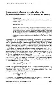
towards the most popular documents, thus approaching a Zipf-like behavior. As far as the topology of the experiments is concerned, regular Qary trees are used in all examples. Regular Q-ary trees are commonly used for the derivation of numerical results for algorithms operating on trees Rodriguez et al., 2001. The entire set of parameters (demand and topology) for each experiment is indicated in the title of the corresponding graph. The distance function dj,v capture the number of hops between client j (co-located with the jth leaf thus dj,j = 0) and node v. The distance of the origin server is dj,os = L for an L level hierarchy. Figure 1 shows the average cost per request for Greedy and iGreedy (expressed in number of hops to reach an object). The performance of the heuristic algorithms is plotted against the bound of the corresponding optimal performance obtained from the LP-relaxation of the ILP of Sect.3.2. The x-axis indicates the number of available storage units in the hierarchy (S) with each storage unit being able to host a single object. From the graph it may be seen that iGreedy is no more than 3% away from the optimal while Greedy may deviate as much as 14% in the presented results. The performance gap between the two owes to the waste of a significant amount of storage in barren objects under Greedy. Figure 2 illustrates the effect of the degree of homogeneity in the access patterns of different clients. Two clients are non-homogeneous if they employ different demand distributions. In the presented results each client j references N objects; βN objects are common to all clients while the remaining (1 − β)N are only referenced by client j. A Zipf-like distribution is created for each client by randomly choosing an object from its reference set and assigning it the next higher value from a Zipflike distribution and then repeating the same action until all objects have been assigned probabilities. The parameter β will be referred to as the overlap degree; values of β approaching 1 mean that most objects are common to all clients (although each client may request a common object with a potentially different probability) while small values of β
PSfrag replacements
Storage Capacity Allocation Algorithms for Hierarchical Content Distribution11 N=10000, S=10000, L=3, Q=4, a=0.7, lambda=ones
N=10000, L=3, Q=2, a=0.9, lambda=ones 1.6
Greedy iGreedy LP relaxation
1.5 1.4 1.3 1.2 1.1 1 0.9
level-1 level-2 level-3
8000 7000 total level capacity
average cost (number of hops)
9000
0.8
6000 5000 4000 3000 2000
0.7
1000
0.6 0.5 1000
2000
3000
4000 5000 6000 7000 8000 S (storage capacity allocated)
9000 10000
0 0.1
0.2
0.3
0.4
0.5 0.6 0.7 β (overlap degree)
0.8
0.9
Figure 2. The effect of non-homogeneous The average cost of Greedy, demand on the per-level allocation of storage iGreedy and LP-relaxation. under iGreedy.
Figure 1.
mean that each client references a potentially different set of objects. Figure 2 shows that the root level (level-3) of a hierarchical system is assigned more storage when there is a substantial amount of overlap in client reference patterns. Otherwise most of the storage goes to the lower levels. This behavior is explained as follows. Storage is effectively utilized at the upper levels when each placed object receives an aggregate request stream from several clients. Such an aggregation may only exist when a substantial amount of objects are common to all clients; otherwise it is better to allocate all the storage to the lower levels – thus sacrificing the (ineffective) aggregation effect – and instead reduce the distance between clients and objects.
4.
CONCLUSIONS
In this paper the storage capacity allocation problem has been considered and a linear time efficient heuristic algorithm, iGreedy, has been developed for its solution. iGreedy has been shown to provide for a good approximation of the optimal by means of numerical comparison against the bound of the optimal (obtained using LP-relaxations).
References Bartal, Y. (1996). On approximating arbitrary metrics by tree metrics. In Proceedings of the 37th Annual IEEE Symposium on Foundations of Computer Science (IEEE FOCS). Breslau, Lee, Cao, Pei, Fan, Li, Philips, Graham, and Shenker, Scott (1999). Web caching and Zipf-like distributions: Evidence and implications. In Proceedings of the Conference on Computer Communications (IEEE Infocom), New York. Cao, Pei and Irani, Sandy (1997). Cost-aware WWW proxy caching algorithms. In Proceedings of the USENIX Symposium on Internet Technologies and Systems, pages 193–206.
1
12 Chesire, Maureen, Wolman, Alec, Voelker, Geoffrey M., and Levy, Henry M. (2001). Measurement and analysis of a streaming-media workload. In Proceedings of USITS. Cormen, Thomas H., Leiserson, Charles E., Rivest, Ronald L., and Stein, Clifford (2001). Introduction to Algorithms, 2nd Edition. MIT Press, Cambridge, Massachusetts. Fan, Li, Cao, Pei, Almeida, Jussara, and Broder, Andrei Z. (2000). Summary cache: a scalable wide-area web cache sharing protocol. IEEE/ACM Transactions on Networking, 8(3):281–293. Gadde, Syam, Chase, Jeff, and Rabinovich, Michael (2002). Web caching and content distribution: A view from the interior. Computer Communications, 24(2). Garces-Erice, Luis, Biersack, Ernst W., Ross, Keith W., Felber, Pascal A., and UrvoyKeller, Guillaume (2003). Hierarchical P2P systems. In Proceedings of ACM/IFIP International Conference on Parallel and Distributed Computing (Euro-Par), Klagenfurt, Austria. Kangasharju, Jussi, Roberts, James, and Ross, Keith W. (2002). Object replication strategies in content distribution networks. Computer Communications, 25(4):376– 383. Kelly, T. and Reeves, D. (2001). Optimal web cache sizing: scalable methods for exact solutions. Computer Communications, 24(2):163–173. Korupolu, Madhukar R., Plaxton, C. Greg, and Rajaraman, Rajmohan (1999). Placement algorithms for hierarchical cooperative caching. In Proceedings of the 10th Annual Symposium on Discrete Algorithms (ACM-SIAM SODA), pages 586 – 595. Krishnan, P., Raz, Danny, and Shavit, Yuval (2000). The cache location problem. IEEE/ACM Transactions on Networking, 8(5):568–581. Laoutaris, Nikolaos, Zissimopoulos, Vassilios, and Stavrakakis, Ioannis (2004a). Joint object placement and node dimensioning for internet content distribution. Information Processing Letters, 89(6):273–279. Laoutaris, Nikolaos, Zissimopoulos, Vassilios, and Stavrakakis, Ioannis (2004b). On the optimization of storage capacity allocation for content distribution. Computer Networks. [submitted]. Li, Bo, Golin, Mordecai J., Italiano, Giuseppe F., Deng, Xin, and Sohraby, Kazem (1999). On the optimal placement of web proxies in the internet. In Proceedings of the Conference on Computer Communications (IEEE Infocom), New York. Pan, Jianping, Hou, Y. Thomas, and Li, Bo (2003). An overview DNS-based server selection in content distribution networks. Computer Networks, 43(6). Rabinovich, Michael (1998). Issues in web content replication. Data Engineering Bulletin (invited paper), 21(4). Ranganathan, K. and Foster, I. (2001). Identifying dynamic replication strategies for a high performance data grid. In Proceedings of the International Workshop on Grid Computing, Denver, Colorado. Rodriguez, Pablo, Spanner, Christian, and Biersack, Ernst W. (2001). Analysis of web caching architectures: Hierarchical and distributed caching. IEEE/ACM Transactions on Networking, 9(4). Saroiu, Stefan, Gummadi, Krishna P., Dunn, Richard J., Gribble, Steven D., and Levy, Henry M. (2002). An analysis of internet content delivery systems. In Proceedings of the 5th Symposium on Operating Systems Design and Implementation (OSDI 2002). Wessels, Duane and Claffy, K. (1998). ICP and the Squid web cache. IEEE Journal on Selected Areas in Communications, 16(3). Williamson, Carey (2002). On filter effects in web caching hierarchies. ACM Transactions on Internet Technology, 2(1).