Sep 10, 1976 - to extract signals from noise (Kalman and Bucy, 1961), and in ... introduce a strong nonlinearity in neuronal interaction, can be treated in an ... A model for a collection of such interacting neurons is given by d ... In an area like cerebral cortex each neuron ... analysis of small vibrations in mechanical systems.
Journal of J. Math. Biology 4, 303--321 (1977)
9 by Springer-Verlag 1977
Storing Covariance With Nonlinearly Interacting Neurons T. J. Sejnowski, Princeton, N. J. Received September 10, 1976
Summary A time-dependent, nonlinear model of neuronal interaction which was probabilistically analyzed in a previous article is shown here to be a natural generalization of the Hartline-Ratliff model of the Limulus retina. Although the primary physical variables in the model are the membrane potentials of neurons, the equations which govern the means and covariances of the membrane potentials are coupled through the average firing rates; as a consequence, the average firing rates control the selective storage and retrieval of covariance information. Motor learning in the cerebellar cox"~exis treated as a problem of covariance storage, and a prediction is made for the underlying synaptic plasticity: the change in synaptic strength between a parallel fiber and a Purkinje cell should be proportional to the covariance between discharges in the parallel fiber and the climbing fiber. Unlike previous proposals for synaptic plasticity, this prediction requires both facilitation and depression to occur (under different conditions) at the same synapse.
Introduction Graded membrane potentials, which are responsible for the spatial summation and temporal integration of electrical activity within neurons, are now believed to play a direct role in local interaction between neurons (Rakic, 1975). Action potentials remain important for many neurons and are the sole means for rapid, long-distance communication. One aim of this article is to physically motivate a model of neuronal interaction which provides a unified treatment of these two electrical potentials. The model is nonlinear and time-dependent, and all the variables appearing in it are operationally defined. The primary physical variable is based on the membrane potential. However, if the firing rates depend linearly on the membrane potentials, then the model, as shown in Part I, is physically equivalent to the Hartline-Ratliff model of the Limulus retina, which can be considered a special case. Because ongoing electrical activity of single neurons has an apparently random character in most parts of the brain, and since in many experiments the main data - - such as average firing rates - - are statistical, a probabilistic analysis of the nonlinear model has been undertaken (Sejnowski, 1976b). The main results are summarized in Part II. If the membrane potentials have a Gaussian distribution, then the equations which govern membrane potential covariances Journ. Math. Biol. 4/4
22
304
T.J. Sejnowski:
represent a linear filter. Identical equations are used in communication theory to extract signals from noise (Kalman and Bucy, 1961), and in systems theory to model and control physical systems (Kalman, Falb, and Arbib, 1969). Unlike a conventional linear filter, however, a neuronal filter is adjustable: its characteristics can be altered by varying the average firing rates of the neurons in the filter. The biological significance of adjustable neuronal filters is discussed in Part III. The main concern of this article is with the long-term storage of covariance information. The cerebellum was chosen as a model system first because of its simple, repetitive, well-studied structure, and second because of recent experimental and theoretical work on cerebellar motor learning with which the present work can be directly compared. The cerebellum is treated as an adaptive filter in Part IV, where the optimal synaptic modification is found using the method of adaptive learning (Tsypkin, 1973). This approach to cerebellar motor learning is similar to that of Marr (1969), but his theory of information processing and his prediction for synaptic plasticity are different. Because the present theory predicts the selective weakening as well as strengthening of synaptic strengths in a balanced combination, the problem of synaptic saturation from random modification is overcome and the entire dynamic range of synaptic strength is always accessible. These results are applied in Part V to covariance storage in other areas of the brain. Although the theory of information processing examined in this article depends fundamentally on the cooperative interaction of many neurons, the implications of the theory can be tested with intracellular recordings from single neurons and from neighboring pairs of neurons. A summary of indirect evidence and the design for a direct experimental test are given in the closing discussion.
I. Nonlinear Model
Many neurons, including a majority of the neurons in the vertebrate retina (Werblin and DoMing, 1969), do not produce an action potential and influence other neurons through continuously graded membrane potentials. In a neuron which does produce an action potential, the membrane potential determines the average firing rate. If the membrane potential is above threshold and the firing rate is well below maximum, then, according to the "slow potential theory" of neuronal interaction as presented by Stevens (1966), a neuron's average firing rate transmits to other neurons a faithful reproduction of its membrane potential, diminished in amplitude but unaltered in shape. A nonlinear version of this "slow potential theory" is given here and developed in greater detail in Appendix 1. One of the simplest linear models for neurons which do not produce action potentials is given by d
vo+ vo = Z/(o b
v b + & L,
(1)
Storing Covariance With Nonlinearly Interacting N e u r o n s
305
where Va are the somatic membrane potentials, ~ is the membrane time constant, Ia are the external input currents, R~ are the effective load resistances, and K~b are dimensionless coupling strengths. Action potentials, which introduce a strong nonlinearity in neuronal interaction, can be treated in an approximate but realistic way. The response of an idealized impulse-producing neuron to a constant input current is shown in Fig. 1. In the absence of action potentials (for example, when the sodium conduction channels are blocked), the membrane potential varies smoothly above the threshold for discharge. Define the effective membrane potential as the membrane potential which would be present in a neuron if the action potential were absent. The firing rate p (~b) of an idealized neuron, which is a function of the effective membrane as shown in Fig. 2, has a sharp threshold and, because of the absolute refractory period, an upper bound.
0
t
(b) V2
t
Fig. 1. (a) The m e m b r a n e potential of an idealized neuron as a function of time in response to a constant input current starting at t = 0. The dashed line represents the effective m e m b r a n e potential which would be present in the absence of action potentials. (b) The m e m b r a n e potential of a second idealized neuron which receives synaptic input from the first, as illustrated in Fig. 3
y (9
Fig. 2. The firing rate p (~b) as a function of effective m e m b r a n e potential q~ for an idealized neuron with firing threshold 0 22*
306
T.J. Sejnowski:
//
V2
v
K21
Fig. 3. Schematic illustration of two neurons with a synaptic connection K21 from the first to the second and with inputs r/1 and qz respectively. Micropipettes record the intracellular membrane potentials 1/1 and 112
For the coupled pair of neurons represented in Fig. 3, repetitive firing of the presynaptic neuron produces a repetitive postsynaptic potential, as shown in Fig. lb. Under steady-state conditions the average postsynaptic potential is constant and, for an idealized neuron, proportional to the firing rate. A model for a collection of such interacting neurons is given by d
T~
(t~a+ t~a = ~ gab lOb (~)b) "~ ~ nab ~b, b
(2)
b
where t/b (t) are the input firing rates, B,b are the input coupling strengths, and
Kab a r e the internal coupling strengths, with units of potential/rate. Because the effective membrane potentials are continuous, this nonlinear model applies equally well to neurons which do not produce action potentials and parts of neurons which interact through graded synapses. Above the threshold for lateral inhibition, the response of the Limulus retina to a steady-state pattern of light is given, to a good approximation, by the Hartline-Ratliff model (1957) 1,.a = ea -- ~ Kab I rb, b
(3)
where r a is the rate of firing of an ommatidium, ea represents the input, and K~b are the inhibitory coefficients. If in the nonlinear model the effective membrane potentials are constant, then they can be eliminated in favor of the firing rates ra = lOa (~ Bab rib -t- ~ K,b rb). (4) b
b
The Hartline-Ratliff equation is equivalent to this equation when p (qS), shown in Fig. 2, is restricted to the approximately linear region above threshold.
Storing Covariance With Nonlinearly Interacting Neurons
307
Although many details of real neurons are not included in the continuous model motivated here, the main results based on it also hold in a more general model, given in Appendix 1, which takes into account axonal latency and dendritic electrotonus. Other factors, such as nonlinear voltage-dependent conductances, will be considered elsewhere. In summary, the highly nonlinear action potential was eliminated by first redefining the membrane potential above the threshold for discharge, and secondly by smoothing the postsynaptic potentials. The nonlinear model (2) based on this effective membrane potential differs from the linear model (1) by an effective nonlinear interaction, as represented in Fig. 2.
H. Probabilistic Analysis The solution of the nonlinear model for a particular input is of less interest than the class of solutions generated by an ensemble of randomly varying inputs. The lowest order moments of the resulting ensemble of solutions contain a concise description of the model's probabilistic structure. The mean of the effective membrane potential is defined as (t) = E
(t),
(5)
where E is the expectation, or ensemble average. By virtue of Eq. (2), the means satisfy d v Z ~a + ~ = Z Ko~ Rb (~bb)+ Z B,b qb, b
(6)
b
where the average firing rates are Rb
= E
(7)
and qb = E t/b. Equations with similar nonlinearities have been investigated by Wilson and Cowan (1968) and Grossberg (1973), who base their models on populations of neurons. The primary variable in their equations is the fraction of neurons in an "excited state". In the present case the membrane potentials of individual neurons are studied and the averages are over ensembles in a probability space rather than over physical populations. In general, the equations for the mean effective membrane potentials are coupled, through the average faring rates R (~b), to equations for the higher moments. Because of membrane potential fluctuations, the average firing rate of a neuron as a function of ~, holding all higher order moments fixed, is smoother than p (~b). For example, Fig. 4 shows R(~) for p (q~) a step function at threshold 0 and with 4~ having Gaussian distribution. The covariance between the effective membrane potentials is defined as Cov (~o (s), ~ (t)) = E (~o (s) - ~o (s)) ( ~ (t) - ~ (t))
(8)
308
T.J. Sejnowski:
and satisfies a nonlinear equation by virtue of Eq. (2). However, an unexpected simplification occurs in the analysis of the covariance equation if a physically reasonable assumption is made concerning the probability distribution of the membrane potentials (Sejnowski, 1976 b). In an area like cerebral cortex each neuron may receive input from thousands of others. By the central limit theorem the sum of a large number of independently random inputs has, under quite general conditions, a Gaussian distribution. If we assume that ~ba (t) are Gaussian processes, then the differences qS, ( t ) - ~, (t) have the same joint distribution as ~b',(t), defined as the solution of T
d
~'~ ~'a -~"~ A ab dP'b+ ~, Bah tl'b, b
b
(9)
where ~/~(t) are Gaussian processes having zero mean and the same covariance as ~/b(t), and Aab-~ K'ab- C~ab, where 6~ is the Kronecker delta and K;b (t) = K,b R~ (~bh (t))
(10)
8 Rb n~ (qSb)= g ~b"
(11)
This equation, which determines the covariance of qS, and will be called the" covariance equation, resembles the linear model for graded electrical coupling (1), with the interaction matrix K'~b playing the role of the linear coupling coefficients. The multiplicative weights R~ appearing in these effective coupling strengths depend on the membrane potentials, as shown in Fig. 4. Those neurons with average membrane potentials near threshold and those connections
RC~I
f @
R'I~)I
o Fig. 4. The average firing rate R (5) and its derivative R' (5) as functions of the mean effective membrane potential 5. The threshold for firing is 0
Storing Covariance With Nonlinearly Interacting Neurons
309
between such critical neurons contribute most effectively to the covariance equation. Despite the linear form of the covariance equation, the coupled equations for the means and covariances are, of course, nonlinear. In the stationary case, the mean membrane potentials are independent of time, the membrane potential covariances depend only on time differences, and the equations for the means and covariances are coupled only through the variances. These equations may have more than one solution (Sejnowski, 1976a). The assumption that the effective membrane potentials are Gaussian can be tested experimentally and enters at the same physical level as the assumptions which led to the nonlinear model. A more general model is given in Appendix 1 which takes into account the random element in spike production and from which it follows as a theorem that the membrane potentials are Gaussian. If the membrane potentials are indeed Gaussian then, because only the first two moments of Gaussian processes are independent, only a small part of all the detailed timing information in afferent spike trains is available for processing by the membrane potentials.
~
V(t)
(o)
r
(b).
(~(t)
(cl
r
(d)
#X
r-. f - .
~
#x
A
[
Fig. 5. Summary diagram of the variables which enter in the analysis of neuronal interaction. (a) The membrane potential V(t) includes action potentials as well as the graded potential. (b) ~b(t) is the effective membrane potential which would be present if the action potential were absent. (c) ~ (t) is the mean effective membrane potential. (d) ~b' (t) is equivalent to the difference q~ (t) - ~ (t) which is quadratically related to the covariance of ~b (t)
310
T.J. Sejnowski:
The nonlinear model of neuronal interaction, summarized in Fig. 5, becomes more linear at each successive stage of probabilistic analysis: (a) The membrane potential, including the highly nonlinear action potential, is the primary variable. (b) A smoother effective membrane potential is introduced which leads to the nonlinear model (2). (c) At the next level the equation (6) for the mean effective membrane potentials is significantly less nonlinear. (d) In the last stage of analysis the covariance equation (9) has a linear form. These last two levels are coupled by the average firing rates (7). III. Neuronal Filters
The covariance equation represents a linear filter whose dimension is equal to the number of neurons in the filter. In some respects the solution of the stationary covariance equation (Sejnowski, 1976 b) resembles the normal mode analysis of small vibrations in mechanical systems. The interacting neurons are particularly sensitive to input covariances with special spatial patterns, which depend on the eigenvectors of the interactions matrix, and special frequencies, which depend on its eigenvalues. However, the normal modes of a mechanical system are derived from a symmetric matrix and are always orthogonal, but the interaction matrix is generally not symmetric and its eigenvectors are generally not orthogonal. As a consequence, coupled covariance modes can appear which correspond to eigenvectors lying in the same direction; when excited, they emerge and decay in sequence. Moreover, the qualitative behavior is same even when the eigenvectors are only approximately degenerate. Because the interaction matrix in the covariance equation depends on R;, the covariance modes of a neuronal filter are adjustable and depend on the average firing rates. Thus, an area of the brain could, through descending , influence on the background firing rates, affect the filter characteristics of a lower processing center. Such an adjustable filter may underlie the ability of an organism to selectively direct its attention and to extract special features from sensory information. Some afferent systems to an area may contribute little to the background firing rates but could have a significant affect on membrane potential covariances. An experiment concerned solely with average firing rates might not detect such an input even if it were a major source of information to the area. Cases of major anatomical pathways without corresponding electrophysiological influence, as judged by average rate, are not uncommon. For example, most ascending projections from thalamic nuclei to cerebral cortex are accompanied by reciprocal corticothalamic tracts, but the electrophysiological influence of these descending projections to the thalamus is weak compared to the influence of other afferents. In the visual system of the cat, the responses of cells in the dorsal lateral geniculate nucleus to spots of light are not affected by cooling visual cortex (Kalil and Chase, 1970). However, for some neurons the cooling had a significant reversible effect on the pattern of impulses in response to moving slits of light. If the primary purpose of descending influence to thalamic relay nuclei is to provide such timing information, then cortical feedback could play an important role in covariance processing.
Storing Covariance With Nonlinearly Interacting Neurons
311
IV. Motor Learning Information processed as membrane potential covarianc~ might be stored in a similar form. The remainder of this article is concerned with covariance storage and its possible relation to learning and memory. In this part cerebellar motor learning is examined, and in the next part the results are applied to other areas of the brain. The cerebellum participates in the control of movement directly through its influence on spinal motoneurons and indirectly through the modification of motor commands from higher centers. Purkinje cells, which provide the only output from the cerebellum, have two main afferent systems, the climbing fibers and the mossy fibers. The entire dentritic tree of a Purkinje cell is entwined by a single climbing fiber. In contrast, mossy fibers branch extensively, each fiber reaching, through granule cells and parallel fibers, thousands of Purkinje cells. A schematic view of a Purkinje cell dendrite is shown in Fig. 6.
pf Pd
CF
Fig. 6. Schematic illustration of a cerebellar Purkinje cell dendrite Pd, a climbing fiber CF (entwining the dendrite trunk), and a parallel fiber pf (passing through the dendrite tree), based on Palay and Chan-Palay (1974). Climbing fiber varicosities make numerous synaptic contacts with spines on the dendritic trunk. The synapse between the parallel fiber and the dendritic branchlet of the Purkinje cell is assumed to vary in strength
It is generally believed that, in coordinating sensory and motor information, the cerebellum uses average rate of firing as its main neural code. Purkinje cells generally have a high spontaneous firing rate of 20 to 100/second, but climbing fibers on average discharge at only 1/second (Eccles, Ito, and SzentSgothai, 1967). Recordings from pairs of nearby climbing fibers show significant correlations lasting more than 100 milliseconds (Bell and Kawasaki, 1972). Thus, the climbing fiber system may be primarily concerned with timing information. The cerebellum is involved in "fine-tuning" the vestibulo-ocular reflex, a compensatory eye movement induced by head rotation (Ito, 1975; Robinson,
312
T.J. Sejnowski:
1976). Because synaptic delays would be greater than the response time of the reflex, no closed-loop feedback from the retina to the vestibular nuclei is possible. However, the cerebellum does receive visual feedback through the climbing fiber system, and the accuracy of the open-loop vestibulo-ocular reflex is improved by visual experience over a time scale of days. Lesion of the vestibulo-cerebellum entirely abolishers this behavioral plasticity. Marr (1969) has proposed a theory for how the cerebellum could learn to perform motor skills. A climbing fiber, according to Marr's explanation, modifies the synapses between the parallel fibers and the Purkinje cell: after being "taught" to activate the Purkinje cells, the same input along the parallel fiber system fires the Purkinje cells without the help of the climbing fiber input. This approach t o motor learning, formulated by Marr entirely within a ratecoded theory of information processing, can be reformulated within the framework of covariance processing. Let ~ba(t) be the effective membrane potentials of all the neurons in the cerebellum, including intrinsic neurons, and let ~/b(t) and r (t) represent the mossy fiber and climbing fiber inputs, with input coupling strengths Bah and Ca respectively. Since each Purkinje cell receives approximately 100,000 synaptic connections from parallel fibers, we can reasonably assume that the membrane potentials of Purkinje cells are Gaussian. Then, following the conventions in Part II, the covariances satisfy d z ~-f (o'a = ~ Aab ~ + ~ Bah tlb + Ca ~'a, (12) b
b
and the part of the covariances ~'a (t) arising from climbing fiber inputs satisfies d "r -dr ~b',,= ~ A ab ~'b + Ca ~'a. (13) b How should the synaptic strengths Ko~ be altered so that membrane potential covariances ~b'a(t) before learning are augmented by a small amount ~ ~O'a (t) after learning has taken place? If the synaptic strengths were altered by a small amount ~ X,b, then Eqs. (12) and (13) require, to first oder in e, that
co r (0 = ~ Kob ~ (0 ~ (0. b
(14)
If the plastic synapses are the ones between parallel fibers and Purkinje cells, then the only contribution to the right side of Eq. (14) are the output covariances from the granule cells. In terms of the firing rates of the granule cells
~o(t) = po (~a (t)),
(15)
the requirement for associative storage becomes C a ~1a (t) - ~ - Z Kab ~b (t), b
(16)
where ~'a(0 and ~(t) are the input covariances to Purkinje cells arising from the climbing fibers and the parallel fibers respectively. Since these are arbitrary temporal processes and ~cab are fixed modifications to the coupling strengths, Eq. (16) can only be approximately satisfied.
Storing CovarianceWith Nonlinearly Interacting Neurons
313
The optimal value of ~ which minimizes the mean square error between the right and left sides of Eq. (16) is found in Appendix 2, but it requires a priori knowledge of the covariances and cannot be practically implemented with neurons. The method of stochastic approximation provides an algorithm for recursively estimating the optimal solution when only sample functions are given (Tsypkin, 1973). The present problem differs from most applications of this method in that the nonlinear background as well as the linear system being optimized depends on the coupling strengths. This difficulty will not be dealt with here; the present treatment is valid only for small changes to the synaptic strengths. The predicted modification to the coupling strengths, derived in Appendix 2, is given by the learning algorithm bCab= 7 S t dt' Ca [~a (t') ~b (t') -- ~a (t') ~b (t')],
(17)
where 7 is a constant. The covariance on the right side is the temporal correlation between the climbing fiber and the parallel fiber relative to the product of their means - - that part of the correlation owing to chance. Notice that, consistent with cerebellar neuroanatomy, a single climbing fiber must be able to influence all the modifiable synapses on a single Purkinje cell. Because the covariance in the learning algorithm can be either positive or negative, the plastic synapse should be capable of both long-term facilitation and depression. In comparison, Marr's theory (1969) only predicts facilitation when there is a "conjunction of presynaptie and climbing fiber (or postsynaptic) activity". Such a plastic synapse eventually reaches maximum strength through chance coincidences, or else loses information by nonspecific decay. The plastic synapse predicted here maintains a constant average strength when the climbing fiber and the parallel fiber are uncorrelated; when these inputs are appropriately correlated the synaptic strength can be flexibly adjusted anywhere within its dynamic range (Sejnowski, 1977).
V. Memory Climbing fibers played an important role in the treatment of covariance storage in the cerebellum. Similar anatomical processes have been found in cerebral cortex by Cajal (1911)~ and more recently Szent~tgothai (1969) has written that "in the Golgi picture it is quite common to see a number of fine terminal axons running for considerable distances closely associated into bundles which in many cases can be seen to contain a dendritic shaft in their axes". Thus, the learning algorithm (17) could also be used for long-term covariance storage in cerebral cortex. There are, however, major differences between the information stored in cerebellar cortex and elsewhere. In the cerebellum, the membrane potential covariances of granule cells depend mainly on the mossy fibers and very little on the climbing fibers. As a consequence, the learning algorithm simply associates the covariances along these two afferent systems. In a more highly interconnected area, such as cerebral cortex, the climbing fiber input could
314
T.J. Sejnowski:
influence neurons which themselves appear on the right side of Eq. (14). Another difference between cerebellar and cerebral cortex lies in the damping time of their covariance modes. The cerebellum participates in ballistic movements such as saccadic eye movements. Long reverberations would not be helpful and might even interfere with the precision timing required for fine control. Parts of the cerebral cortex are concerned with coordination on a longer time scale and can be expected to have a corresPondingly longer coherence time for membrane potential correlations. A component of short-term memory is believed to depend on electrical reverberations, though it is not known what physical aspects of transient electrical activity are involved. If the covariance modes of the brain had a sufficiently long coherence time, then membrane potential covariance could serve as the physical basis for short-term memory. Temporary storage of information, however, is likely to be the result of not one but several interacting control processes. For example, any means for maintaining or reproducing the background firing rates in an area would preserve its covariance modes. Short-term changes to the strengths of synapses may also be important. A neuronal filter already has some of the properties which would be desirable for long-term memory. The processing is distributed in a large collection of neurons, and information can be retrieved a s temporal sequences of covariance modes. A neuronal filter has the additional advantage that different covariance modes can be selected by adjusting the background firing rates of the neurons. The cerebral cortex receives inputs from thalamic nuclei, association fibers from other cortical areas, commisural fibers from the corpus collosum, and a variety of other afferents from the brain stem, basal ganglia, and elsewhere. The background firing rates in a cortical area could be controlled by several of these afferent systems, one part arising from general arousal and another part from a specific sensory modality. Other afferents may be primarily concerned with processing covariance information. For example, consider visual cortex. Under normal conditions the background firing rates of neurons in a high-order visual area depend mainly on sensory input. Imagine that covariance information, perhaps from other sensory modalities, is stored while viewing a particular scene. If subsequently another afferent system could, in the absence of visual input, reestablish the same or similar background firing rates, then the stored covariances could be retrieved and used for further processing. Visual associations may be stored in this manner for many different visual scenes, each corresponding to a different set of background firing rates. The synaptic plasticity predicted from the learning algorithm is small and occurs slowly compared to dynamic time scales. For a stable solution of the nonlinear model, small changes to synaptic strengths cause correspondingly small changes in covariance processing (Sejnowski, 1976 b). However, if the interaction matrix has eigenvalues with real parts near one, then the solution is nearly unstable and a small change to synaptic strengths could produce a large change to the coupled nonlinear equations (Sejnowski, 1976a).
Storing Covariance With Nonlinearly Interacting Neurons
315
In summary, the background firing rates determine the covariance modes in an area, but only those modes which are persistently excited by incoming correlations are strengthened. How synaptic modification affects previously stored information is examined in Appendix 2. Discussion
Because an impulse-producing neuron is maximally sensitive to input correlations when its average membrane potential is near threshold, neurons which process covariance information must maintain a moderate rate of firing. The levels of spontaneous activity found in many parts of the nervous system meet this requirement. There is in fact some indirect evidence for the sensory coding of correlations and the use of correlation information in the auditory, somatosensory, and visual systems. In the auditory system, phase information in the phase-locked discharges between the two ears is used for low-frequency binaural localization (Jeffress, 1975). Temporal information in the auditory nerve discharges may also have an important role in pitch perception (Plomp, 1975). In the somatosensory system, information coded as interspike intervals can apparently be used for perceiving the frequency of flutter-vibration (Mountcastle, 1967), and some central neurons fire with preferred interspike intervals even under normal conditions (Amassian and Giblin, 1974). In the visual system, random-dot stereograms, which have a random texture when viewed monocularly, are perceived in depth if the dots are binocularly correlated either spatially (Julesz, 1971) or temporally (Ross, 1974). Simultaneous recordings of spike trains have been obtained from pairs of neurons in the retina (Rodiek, t967), the lateral geniculate nucleus (Stevens and Gerstein, 1976), the cerebellum (Bell and Kawasaki, 1972), the auditory cortex (Dickson and Gerstein, 1972), and elsewhere. The spike trains in many cases were significantly correlated. Viewed from the present perspective, the question of whether the correlations were produced by direct interaction or a common input is secondary to the question of whether large-scale correlations exist and are related to sensory processing. Since in most neurons the membrane potential is often below the threshold for producing impulses, correlations between membrane potentials should be at least as prominent as the correlations found between spike trains. The significance of correlations between membrane potentials for sensory processing can be investigated with intracellular recording. An ensemble of intracellular records from a pair of neurons responding to a controlled sensory stimulus could be used to determine the means and covariance of the membrane potentials and to test the assumption that membrane potentials are approximately Gaussian. The long-term storage of covariance information depends on synaptic plasticity similar to that proposed by Hebb (1949), Marr (1969), and Stent (1973). The strict balance between facilitation and depression required by the present
316
T.J. Sejnowski:
prediction distinguishes it from other proposals (Sejnowski, 1977). As a consequence, the average strength of a plastic synapse cannot be altered by simply increasing the firing rate of the climbing fiber or the parallel fiber. For the synaptic strength to vary, the impulses in these two afferents must occur in coincidence more often or less often than by chance. The next step toward describing biological reality is the detailed modeling of specific areas. Unless our understanding of basic neuronal function is seriously in error, the nonlinear model analyzed here should provide a reasonably good first approximation. The remarkable parallels with communication and systems engineering could prove useful not only in analyzing experimental data but as well in understanding the design principles of the nervous system.
Acknowledgement I am especially grateful to David Bender, Bruce Knight, Jr., and Murray Lampert for helpful discussions and useful suggestions.
Appendix 1. Point Process Model The results of this article are based on the model of neuronal interaction which was motivated in Part I. This continuous model is derived here from a point-process model, and the variables in both models are given precise interpretations. A spike train, regarded as a sequence of points in time, can be modeled by a stochastic point process on the real line (Snyder, 1975). Let N (t) represent the number of spikes on time interval [0, t). Assume that the mean number of spikes E N (t) is differentiable, and define the "instantaneous average rate" (t) =
d
E N (0.
(18)
For example, consider the case when the point process is Poisson. Then the probability that there are n spikes on the interval [0, t) is
P (N(t)= n) = (n!) - t A (t)" e -a('),
(1.9)
with A (t) =
at'
(t').
Since the mean number of spikes on the interval is E N (t)= A (t), the "instantaneous average rate" is t/(t)= ). (t). This interpretation of 17(t) is related to the "instantaneous rate", an experimental variable which has been useful in measuring the dynamic response of the Limulus retina (Ratliff, 1974). Given a spike train with spikes at times {rl}, the "instantaneous rate" is defined as a(t)=(t i+l-ti)-t,
t i < t _ < t I+1.
(20)
Storing Covariance With Nonlinearly Interacting Neurons
317
S(t)
II
t
Nit)
I-
1
S
~(t)
L t
Fig. 7. A typical spike train S (t) as a function of time, the cumulative number of spikes N (t), and the "instantaneous rate" a (t), defined by Eq. (20) It is a p p a r e n t f r o m Fig. 7 t h a t
~6 dt' ~ (t') = N (t) + e (t) w h e r e the e r r o r is b o u n d e d ] e (t) ] < 1 a n d E ~ (t) = 0. C o n s e q u e n t l y , the a v e r a g e o f t h e " i n s t a n t a n e o u s r a t e " o v e r a n e n s e m b l e of i d e n t i c a l l y p r e p a r e d e x p e r i m e n t s gives an e s t i m a t e for the " i n s t a n t a n e o u s a v e r a g e r a t e " d N ~ ( t ) : 27E (t):,l(t).
:r
(21) t
t
~p-ac
~
t
Fig. 8. Idealized intracellular recording of the membrane potential x (t) as a function of time. Upon reaching threshold, an impulse is released and the membrane potential is reset to a lower potential. In contrast, the effective membrane potential 0 (t), which does not include the impulse or reset, is continuous. The difference 0 (t)-x(t) suffers a step discontinuity which damps exponentially
318
T.J. Sejnowski:
The "effective membrane potential" which was motivated in Part I can now be more precisely defined. Let ~k (t) be the membrane potential of a neuron which does not produce an action potential but which receives a spike train as input. Then the membrane potential satisfies the stochastic differential equation
0 (t) + 0 (t) dt = B d N (t),
(22)
where B ist the jump in the postsynaptic potential from a single synaptic event. The effect of spike production on the membrane potential is shown in Fig. 8: the difference between the membrane potential with and without reset exponentially damps after each impulse. The average of Eq. (22) over an ensemble of point processes is d z ~- ~b (t) + ~ (t) = n t/(t),
(23)
where the average membrane potential q ~ ( t ) = E ~ ( 0 corresponds to the "effective membrane potential" motivated in Part I. The resemblance between Eq. (23) and the continuous model (2) further suggests that p (0), previously defined as the firing rate to a constant input current, should be interpreted as an "instantaneous average rate". Thus, a natural generalization of the continuous model is given by the stochastic integral equation t
t
Oa(t)=~. ~ Kab(t,t')dMb(t')+~, b
~ U,b(t,t')dNb(t'),
(24)
b
where the point processes d M b and d N b satisfy d d--f E Mb (t) = Pb (~b (t)), d d-T E n b (t) = ~/b(t).
(25) (26)
The kernel K~b (t, t') is the temporal response of ~ (t) to an impulse at time t' from a neighboring neuron, and B~b (t, t') the response to an impulse from an external input. Since ~a(t) and t/b(t) are themselves stochastic processes, the point processes i n Eq. (24) are doubly stochastic (Snyder, 1975). If a neuron receives many Poisson inputs, then by a central limit theorem its membrane potential is approximately Gaussian. The time-dependent coupling kernels in this point-process model take into account the electrical properties of the intervening axons, synapses, and dendrites. The special case 1
K,b (t, t') -= ~- Kab e -(t-t')/~ corresponds to the simple model of exponential decay considered in Part I.
(27)
Storing Covariance With Nonlinearly Interacting Neurons
319
2. Covariance Storage and Retrieval Covariance storage was on the modification of given here, together with of covariance storage on
examined in Part IV where conditions were derived the synaptic strengths. The optimal modification is an approximate algorithm for achieving it. The effect previously stored information is also considered.
Given the zero-mean processes ~'a (t) and ~, (t) on the time interval [0, T), the problem is to find K,b which minimizes the mean square error T
gT (Kab) E S dt ~, e2a(t),
(28)
=
0
a
where e.
(t) =
C a ~a (t) -- 2 Kab ~tb (t). b
(29)
The minimum occurs when the variation of ~ r (Nab) with respect to X~b vanishes. The result is
K*b (7) = C~ ~c
dt Cov (~'a (t), ~; (t)
9
dt Cov (~; (t), ~; (t))
.
(30)
In the stationary case ~c*b (7) is independent of T. Stochastic approximation is a constructive method for estimating the optimal solution given only sample functions of the processes (Tsypkin, 1973). The adaptive learning algorithm for the present problem is d d t ~,b = 7 C, [Cov (~'~(t), ~; (t)) - ~ x,c Coy (~'c(t), ~; (t))],
(31)
r
where 7 is a positive constant (or a negative constant if the associative storage is complementary). The magnitude of 7, corresponding to the efficiency of plasticity, is sufficiently small to insure convergence of ~ab to ~Ca*b,and sufficiently large to do so in a reasonable time. If 1cab is small, as assumed in Part IV, then the second term of Eq. (31) can be neglected, leaving d d t tcab= 7 Ca Cov (~', (t), ~; (t)).
(32)
Notice that the integrated form of this approximate learning algorithm is proportional to the first factor of the optimal solution it*b in Eq. (30) (Pfaffelhuber, 1975). When only sample functions are given, the covariance may be approximated by d d~- K"b= 7 C, [r (t) ~b (t) - ~a (t) ~b (t)],
(33)
and the learning algorithm (17) follows by a simple integration. Let us now examine how information stored by this learning algorithm is retrieved. Consider the stationary case for which the solution to the covariance equation is (Sejnowski, 1976b) Journ. Math. Biol. 4/4
23
320
T.J. Sejnowski: t
~b'a(0 = ~
S & ' T~b ( t - - t ' ) B ~ q ' ~ (t'),
(34)
be
where Tab(t--t' ) is the transition equation is
matrix.
The
Laplace transform
~[4al =Y, ~[Lb] Bbc ~e[.;].
of this
(35)
bc
If the perturbation of the interaction matrix 6 K~,b is sufficiently small, then the effect on the transition matrix, to first order in the perturbation (Sejnowski, 1976a), is given by 6 &o [Tab] = ~
&a [T~]
6 K;e &~o[Tab].
(36)
cd
The o u t p u t perturbation obtained from Eq. (35) is ~ [ 4 ; ] = ~ La [Tab] 6 K;c ~ [q~;].
(37)
bc
C o m p a r i s o n of Eq. (35) with Eq. (37) reveals that the perturbation of the o u t p u t is equivalently p r o d u c e d by
Z Bbc b tl; (t) = Z 6 Kb~ R'~ (t) ~)" (t). c
(38)
c
That is, after the p e r m a n e n t change b Kb~ has been made to the coupling strengths, the inputs are effectively augmented by this added component. Notice that the effective input perturbation depends only on the output, and that it resembles the condition (14) for synaptic modification. This last result (38) is also valid for the nonstationary case and follows directly from the covariance equation. References
Amassian, V. H., Giblin, D. : Periodic components in steady-state activity of cuneate neurones and their possible role in sensory coding. J. Physiol. 243, 353--385 (1974). Bell, C., C., Kawasaki, T.: Relation among climbing fiber responses of nearby Purkinje ceils. J. Neurophysiol. 35, 155--169 (1972). Dickson, J. W., Gerstein, G. L. : Interactions between neurons in auditory cortex of the cat. J. Neurophysiol. 37, 1239--1261 (1974). Eccles, J. C., Ito, M., Szent~tgothai, J. : The cerebellum as a neuronal machine. Berlin-HeidelbergNew York: Springer 1967. Grossberg, S. : Control enhancement, short-term memory, and constancies in reverberating neural networks. Studies in App. Math. 52, 213--257 (1973). Hartline, H. K., Ratliff, F.: Inhibitory interaction of the receptor units in the eye of Limulus. J. Gen. Physiol. 40, 1357--1376 (1957). Hebb, D. O. : The organization of behavior. New York: Wiley 1949~ Ito, M. : Learning control mechanisms by the cerebellum flocculo-vestibulo-ocular system. In: The nervous system, Vol. 1 (Tower, D. H., ed.). New York: Raven Press 1975. Jeffress, L. A.: Localization of sound. In: Handbook of sensory physiology V/2: Auditory system (Keidel, W. D., Neff, W. D., eds.). Berlin-Heidelberg-New York: Springer 1975. Julesz, B. :Foundations of cyclopean perception. Chicago: University of Chicago Press 1971. Kalil, R. E., Chase, R. : Corticofugal influence on activity of lateral geniculate neurons in the cat. J. Neurophysiol. 33, 459~74 (1970). Kalman, R. E., Buey, R. S.: New results in linear filtering and prediction theory. J. Basic Engineering 83D, 95--108 (1961).
Storing Covariance With Nonlinearly Interacting Neurons
321
Kalman, R. E., Falb, P. L., Arbib, M. A. : Topics in mathematical system theory. New York: McGraw-Hill 1969. Marr, D. : A theory of cerebellar cortex. J. Physiol. 202, 4 3 7 4 7 0 (1969). Mountcastle, V. B.: The problem of sensing and neural coding. In: The neurosciences: a study program (Quarton, G. C., Melnechuk, T., Schmitt, F. O., eds.). New York: The Rockefeller University Press 1967. Palay, S. L., Chan-Palay, W.: Cerebellar cortex: cytology and organization. Berlin-HeidelbergNew York: Springer 1974. Pfaffelhuber, E. : Correlation memory models - - a first approximation in a general learning scheme. Biol. Cybernetics 18, 217--223 (1975). Plomp, R. : Auditory psychophysics. Ann. Rev. Psychol. 26, 207--232 (1975). Rakic, P. : Local circuit neurons. Neuroscience Res. Prog. Bull. 13, 2 8 9 4 4 6 (1975). Ram6n y CajaI, S.: Histologie du syst6me nerveux de l'homme et des vert6br6s, Tom. II. Paris: Maloine 1955. Madrid: Consejo Superior de Investigaciones Cientificas 1911. Ratliff, F. : Studies in excitation and inhibition in the retina. New York: The Rockefeller University Press 1974. Robinson, D. A.: Adaptive gain control of vestibulo-ocular reflex by the cerebellum. J. Neurophysiol. 39, 954~969 (1976). Rodiek, R. W. : Maintained activity of eat retinal ganglion cells. J. Neurophysiol. 30, 1043--1071 (1967). Ross, J. : Stereopsis by binocular delay. Nature 248, 363--364 (1974). Sejnowski, T. J. : On global properties of neuronal interaction. Biol. Cybernetics 22, 85--95 (1976). Sejnowski, T. J. : On the stochastic dynamics of neuronal interaction. Biol. Cybernetics 22, 203--2t 1 (1976). Sejnowski, T. J.: Statistical constraints on synaptic plasticity. J. Theor. Bio., in press (1977). Snyder, D. L.: Random point processes. New York: Wiley 1975. Stent, G. S. : A physiological mechanism for Hebb's postulate of learning. Proe. Nat. Acad. Sci. U.S.A. 70, 997--1001 (1973). Stevens, C. F. : Neurophysiology: A primer. New York: J. Wiley 1966. Stevens, J. K., Gerstein, G. L. : Interactions between cat lateral geniculate neurons. J. Neurophysiol. 39, 239--256 (1976). Szent~gothai, J. : Architecture of the cerebral cortex. In: Basic mechanisms of the epilepsies (Jasper, H. H., Ward, A. A., Pope, A., eds.). Boston: Little, Brown 1969. Tsypkin, Ya. Z. : Foundations of the theory of learning systems. New York: Academic Press 1973. Werblin, F. S., DoMing, J. E. : Organization of the retina of the mudpuppy, Necturus maculosus: Ii. Intracellular recording. J. Neurophysiol. 32, 339--355 (1969). Wilson, H. R., Cowan, J. D. : Excitatory and inhibitory interactions in localized populations of model neurons. Biophys. J. 12, 1--24 (1972). Dr. T. J. Sejnowski Joseph Henry Laboratories Department of Physics Princeton University Princeton, NJ 08540, U. S. A.
23*