Structural Concepts and Systems for Architects

Draft

DRAFT

Lecture Notes in: STRUCTURAL CONCEPTS AND SYSTEMS FOR ARCHITECTS

Victor E. Saouma Dept. of Civil Environmental and Architectural Engineering University of Colorado, Boulder, CO 80309-0428

Draft Contents 1 INTRODUCTION 1.1 Science and Technology . . . . . . 1.2 Structural Engineering . . . . . . . 1.3 Structures and their Surroundings 1.4 Architecture & Engineering . . . . 1.5 Architectural Design Process . . . 1.6 Architectural Design . . . . . . . . 1.7 Structural Analysis . . . . . . . . . 1.8 Structural Design . . . . . . . . . . 1.9 Load Transfer Mechanisms . . . . 1.10 Structure Types . . . . . . . . . . 1.11 Structural Engineering Courses . . 1.12 References . . . . . . . . . . . . . .

. . . . . . . . . . . .

. . . . . . . . . . . .

. . . . . . . . . . . .

. . . . . . . . . . . .

. . . . . . . . . . . .

. . . . . . . . . . . .

. . . . . . . . . . . .

. . . . . . . . . . . .

. . . . . . . . . . . .

. . . . . . . . . . . .

. . . . . . . . . . . .

2 LOADS 2.1 Introduction . . . . . . . . . . . . . . . . . . . . . . . . 2.2 Vertical Loads . . . . . . . . . . . . . . . . . . . . . . . 2.2.1 Dead Load . . . . . . . . . . . . . . . . . . . . 2.2.2 Live Loads . . . . . . . . . . . . . . . . . . . . E 2-1 Live Load Reduction . . . . . . . . . . . . . . . 2.2.3 Snow . . . . . . . . . . . . . . . . . . . . . . . . 2.3 Lateral Loads . . . . . . . . . . . . . . . . . . . . . . . 2.3.1 Wind . . . . . . . . . . . . . . . . . . . . . . . E 2-2 Wind Load . . . . . . . . . . . . . . . . . . . . 2.3.2 Earthquakes . . . . . . . . . . . . . . . . . . . . E 2-3 Earthquake Load on a Frame . . . . . . . . . . E 2-4 Earthquake Load on a Tall Building, (Schueller 2.4 Other Loads . . . . . . . . . . . . . . . . . . . . . . . . 2.4.1 Hydrostatic and Earth . . . . . . . . . . . . . . E 2-5 Hydrostatic Load . . . . . . . . . . . . . . . . . 2.4.2 Thermal . . . . . . . . . . . . . . . . . . . . . . E 2-6 Thermal Expansion/Stress (Schueller 1996) . . 2.4.3 Bridge Loads . . . . . . . . . . . . . . . . . . . 2.4.4 Impact Load . . . . . . . . . . . . . . . . . . . 2.5 Other Important Considerations . . . . . . . . . . . . 2.5.1 Load Combinations . . . . . . . . . . . . . . . . 2.5.2 Load Placement . . . . . . . . . . . . . . . . .

. . . . . . . . . . . .

. . . . . . . . . . . .

. . . . . . . . . . . .

. . . . . . . . . . . .

. . . . . . . . . . . .

. . . . . . . . . . . .

. . . . . . . . . . . .

. . . . . . . . . . . .

. . . . . . . . . . . .

. . . . . . . . . . . .

. . . . . . . . . . . .

. . . . . . . . . . . .

15 15 15 15 16 16 17 17 17 18 18 25 27

. . . . . . . . . . . . . . . . . . . . . . . . . . . . . . . . . . . . . . . . . . . . 1996) . . . . . . . . . . . . . . . . . . . . . . . . . . . . . . . . . . . . . . . .

. . . . . . . . . . . . . . . . . . . . . .

. . . . . . . . . . . . . . . . . . . . . .

. . . . . . . . . . . . . . . . . . . . . .

. . . . . . . . . . . . . . . . . . . . . .

. . . . . . . . . . . . . . . . . . . . . .

. . . . . . . . . . . . . . . . . . . . . .

. . . . . . . . . . . . . . . . . . . . . .

. . . . . . . . . . . . . . . . . . . . . .

. . . . . . . . . . . . . . . . . . . . . .

. . . . . . . . . . . . . . . . . . . . . .

. . . . . . . . . . . . . . . . . . . . . .

29 29 29 30 30 32 33 33 33 39 40 44 45 47 47 47 48 48 49 49 49 49 50

. . . . . . . . . . . .

. . . . . . . . . . . .

. . . . . . . . . . . .

Draft CONTENTS 5.4

5

Flexure . . . . . . . . . . . . . . . . . . . . . . . . . . . . . . . . 5.4.1 Basic Kinematic Assumption; Curvature . . . . . . . . . . 5.4.2 Stress-Strain Relations . . . . . . . . . . . . . . . . . . . . 5.4.3 Internal Equilibrium; Section Properties . . . . . . . . . . 5.4.3.1 ΣFx = 0; Neutral Axis . . . . . . . . . . . . . . . 5.4.3.2 ΣM = 0; Moment of Inertia . . . . . . . . . . . 5.4.4 Beam Formula . . . . . . . . . . . . . . . . . . . . . . . . E 5-10 Design Example . . . . . . . . . . . . . . . . . . . . . . . 5.4.5 Approximate Analysis . . . . . . . . . . . . . . . . . . . . E 5-11 Approximate Analysis of a Statically Indeterminate beam

. . . . . . . . . .

. . . . . . . . . .

. . . . . . . . . .

. . . . . . . . . .

. . . . . . . . . .

. . . . . . . . . .

. . . . . . . . . .

. . . . . . . . . .

. . . . . . . . . .

112 112 113 113 113 114 114 116 117 117

. . . . . .

. . . . . .

. . . . . .

. . . . . .

. . . . . .

. . . . . .

. . . . . .

. . . . . .

. . . . . .

. . . . . .

123 123 126 126 127 129 129

7 A BRIEF HISTORY OF STRUCTURAL ARCHITECTURE 7.1 Before the Greeks . . . . . . . . . . . . . . . . . . . . . . . . . . . 7.2 Greeks . . . . . . . . . . . . . . . . . . . . . . . . . . . . . . . . . 7.3 Romans . . . . . . . . . . . . . . . . . . . . . . . . . . . . . . . . 7.4 The Medieval Period (477-1492) . . . . . . . . . . . . . . . . . . . 7.5 The Renaissance . . . . . . . . . . . . . . . . . . . . . . . . . . . 7.5.1 Leonardo da Vinci 1452-1519 . . . . . . . . . . . . . . . . 7.5.2 Brunelleschi 1377-1446 . . . . . . . . . . . . . . . . . . . . 7.5.3 Alberti 1404-1472 . . . . . . . . . . . . . . . . . . . . . . 7.5.4 Palladio 1508-1580 . . . . . . . . . . . . . . . . . . . . . . 7.5.5 Stevin . . . . . . . . . . . . . . . . . . . . . . . . . . . . . 7.5.6 Galileo 1564-1642 . . . . . . . . . . . . . . . . . . . . . . . 7.6 Pre Modern Period, Seventeenth Century . . . . . . . . . . . . . 7.6.1 Hooke, 1635-1703 . . . . . . . . . . . . . . . . . . . . . . . 7.6.2 Newton, 1642-1727 . . . . . . . . . . . . . . . . . . . . . . 7.6.3 Bernoulli Family 1654-1782 . . . . . . . . . . . . . . . . . 7.6.4 Euler 1707-1783 . . . . . . . . . . . . . . . . . . . . . . . 7.7 The pre-Modern Period; Coulomb and Navier . . . . . . . . . . . 7.8 The Modern Period (1857-Present) . . . . . . . . . . . . . . . . . 7.8.1 Structures/Mechanics . . . . . . . . . . . . . . . . . . . . 7.8.2 Eiffel Tower . . . . . . . . . . . . . . . . . . . . . . . . . . 7.8.3 Sullivan 1856-1924 . . . . . . . . . . . . . . . . . . . . . . 7.8.4 Roebling, 1806-1869 . . . . . . . . . . . . . . . . . . . . . 7.8.5 Maillart . . . . . . . . . . . . . . . . . . . . . . . . . . . . 7.8.6 Nervi, 1891-1979 . . . . . . . . . . . . . . . . . . . . . . . 7.8.7 Khan . . . . . . . . . . . . . . . . . . . . . . . . . . . . . 7.8.8 et al. . . . . . . . . . . . . . . . . . . . . . . . . . . . . . .

. . . . . . . . . . . . . . . . . . . . . . . . . .

. . . . . . . . . . . . . . . . . . . . . . . . . .

. . . . . . . . . . . . . . . . . . . . . . . . . .

. . . . . . . . . . . . . . . . . . . . . . . . . .

. . . . . . . . . . . . . . . . . . . . . . . . . .

. . . . . . . . . . . . . . . . . . . . . . . . . .

. . . . . . . . . . . . . . . . . . . . . . . . . .

. . . . . . . . . . . . . . . . . . . . . . . . . .

. . . . . . . . . . . . . . . . . . . . . . . . . .

133 133 133 135 136 138 138 139 140 140 142 142 144 144 145 147 147 149 150 150 150 150 151 151 152 152 153

6 Case Study II: GEORGE WASHINGTON BRIDGE 6.1 Theory . . . . . . . . . . . . . . . . . . . . . . . . . . . 6.2 The Case Study . . . . . . . . . . . . . . . . . . . . . . 6.2.1 Geometry . . . . . . . . . . . . . . . . . . . . . 6.2.2 Loads . . . . . . . . . . . . . . . . . . . . . . . 6.2.3 Cable Forces . . . . . . . . . . . . . . . . . . . 6.2.4 Reactions . . . . . . . . . . . . . . . . . . . . .

Victor Saouma

. . . . . .

. . . . . .

. . . . . .

. . . . . .

. . . . . .

Structural Concepts and Systems for Architects

Draft CONTENTS

7

12 PRESTRESSED CONCRETE 12.1 Introduction . . . . . . . . . . . . . . 12.1.1 Materials . . . . . . . . . . . 12.1.2 Prestressing Forces . . . . . . 12.1.3 Assumptions . . . . . . . . . 12.1.4 Tendon Configuration . . . . 12.1.5 Equivalent Load . . . . . . . 12.1.6 Load Deformation . . . . . . 12.2 Flexural Stresses . . . . . . . . . . . E 12-1 Prestressed Concrete I Beam 12.3 Case Study: Walnut Lane Bridge . . 12.3.1 Cross-Section Properties . . . 12.3.2 Prestressing . . . . . . . . . . 12.3.3 Loads . . . . . . . . . . . . . 12.3.4 Flexural Stresses . . . . . . .

. . . . . . . . . . . . . .

. . . . . . . . . . . . . .

. . . . . . . . . . . . . .

. . . . . . . . . . . . . .

197 197 197 200 200 200 200 202 202 204 206 206 208 209 209

13 ARCHES and CURVED STRUCTURES 13.1 Arches . . . . . . . . . . . . . . . . . . . . . . . . . . . . . . . . . . . . . . . 13.1.1 Statically Determinate . . . . . . . . . . . . . . . . . . . . . . . . . . E 13-1 Three Hinged Arch, Point Loads. (Gerstle 1974) . . . . . . . . . . . E 13-2 Semi-Circular Arch, (Gerstle 1974) . . . . . . . . . . . . . . . . . . . 13.1.2 Statically Indeterminate . . . . . . . . . . . . . . . . . . . . . . . . . E 13-3 Statically Indeterminate Arch, (Kinney 1957) . . . . . . . . . . . . . 13.2 Curved Space Structures . . . . . . . . . . . . . . . . . . . . . . . . . . . . . E 13-4 Semi-Circular Box Girder, (Gerstle 1974) . . . . . . . . . . . . . . . 13.2.1 Theory . . . . . . . . . . . . . . . . . . . . . . . . . . . . . . . . . . 13.2.1.1 Geometry . . . . . . . . . . . . . . . . . . . . . . . . . . . . 13.2.1.2 Equilibrium . . . . . . . . . . . . . . . . . . . . . . . . . . . E 13-5 Internal Forces in an Helicoidal Cantilevered Girder, (Gerstle 1974)

. . . . . . . . . . . .

. . . . . . . . . . . .

. . . . . . . . . . . .

211 211 214 214 215 217 217 220 220 222 222 223 224

. . . . . . . . . . . . . .

. . . . . . . . . . . . . .

. . . . . . . . . . . . . .

. . . . . . . . . . . . . .

. . . . . . . . . . . . . .

. . . . . . . . . . . . . .

. . . . . . . . . . . . . .

. . . . . . . . . . . . . .

14 BUILDING STRUCTURES 14.1 Introduction . . . . . . . . . . . . . . . . . . . . . . 14.1.1 Beam Column Connections . . . . . . . . . 14.1.2 Behavior of Simple Frames . . . . . . . . . 14.1.3 Eccentricity of Applied Loads . . . . . . . . 14.2 Buildings Structures . . . . . . . . . . . . . . . . . 14.2.1 Wall Subsystems . . . . . . . . . . . . . . . 14.2.1.1 Example: Concrete Shear Wall . . 14.2.1.2 Example: Trussed Shear Wall . . 14.2.2 Shaft Systems . . . . . . . . . . . . . . . . . 14.2.2.1 Example: Tube Subsystem . . . . 14.2.3 Rigid Frames . . . . . . . . . . . . . . . . . 14.3 Approximate Analysis of Buildings . . . . . . . . . 14.3.1 Vertical Loads . . . . . . . . . . . . . . . . 14.3.2 Horizontal Loads . . . . . . . . . . . . . . . 14.3.2.1 Portal Method . . . . . . . . . . . E 14-1 Approximate Analysis of a Frame subjected 14.4 Lateral Deflections . . . . . . . . . . . . . . . . . . Victor Saouma

. . . . . . . . . . . . . .

. . . . . . . . . . . . . .

. . . . . . . . . . . . . .

. . . . . . . . . . . . . .

. . . . . . . . . . . . . .

. . . . . . . . . . . . . .

. . . . . . . . . . . . . .

. . . . . . . . . . . . . .

. . . . . . . . . . . . . .

. . . . . . . . . . . . . .

. . . . . . . . . . . . . .

. . . . . . . . . . . . . .

. . . . . . . . . . . . . .

. . . . . . . . . . . . . . . . . . . . . . . . . . . . . . . . . . . . . . . . . . . . . . . . . . . . . . . . . . . . . . . . . . . . . . . . . . . . . . . . . . . . . . . . . . . . . . . . . . . . . . . . . . . . . . . . . . . . . . . . . . . . . . . . . . . . . . . . . . . . . . . . . . . . . . . . . . . . . . . . . . . . . . . . . . . . . . . . . . . . . . . . . . . . . . . . . . . . . . . . . . . . . . . . . . . . . . . . . . . . . . . . . to Vertical and Horizontal . . . . . . . . . . . . . . .

229 . . 229 . . 229 . . 229 . . 230 . . 233 . . 233 . . 233 . . 235 . . 236 . . 236 . . 237 . . 238 . . 239 . . 241 . . 241 Loads243 . . 253


Draft List of Figures 1.1 1.2 1.3 1.4 1.5 1.6 1.7 1.8 1.9

Types of Forces in Structural Elements (1D) . Basic Aspects of Cable Systems . . . . . . . . Basic Aspects of Arches . . . . . . . . . . . . Types of Trusses . . . . . . . . . . . . . . . . Variations in Post and Beams Configurations Different Beam Types . . . . . . . . . . . . . Basic Forms of Frames . . . . . . . . . . . . . Examples of Air Supported Structures . . . . Basic Forms of Shells . . . . . . . . . . . . . .

. . . . . . . . .

. . . . . . . . .

. . . . . . . . .

. . . . . . . . .

. . . . . . . . .

. . . . . . . . .

. . . . . . . . .

. . . . . . . . .

. . . . . . . . .

2.1 2.2 2.3 2.4 2.5 2.6 2.7 2.8 2.9 2.10 2.11 2.12 2.13 2.14 2.15 2.16 2.17 2.18

Approximation of a Series of Closely Spaced Loads . . . . . . . Snow Map of the United States, ubc . . . . . . . . . . . . . . . Loads on Projected Dimensions . . . . . . . . . . . . . . . . . . Vertical and Normal Loads Acting on Inclined Surfaces . . . . Wind Map of the United States, (UBC 1995) . . . . . . . . . . Effect of Wind Load on Structures(Schueller 1996) . . . . . . . Approximate Design Wind Pressure p for Ordinary Wind Force Vibrations of a Building . . . . . . . . . . . . . . . . . . . . . . Seismic Zones of the United States, (UBC 1995) . . . . . . . . Earth and Hydrostatic Loads on Structures . . . . . . . . . . . Truck Load . . . . . . . . . . . . . . . . . . . . . . . . . . . . . Load Placement to Maximize Moments . . . . . . . . . . . . . . Load Life of a Structure, (Lin and Stotesbury 1981) . . . . . . Concept of Tributary Areas for Structural Member Loading . . One or Two Way actions in Slabs . . . . . . . . . . . . . . . . . Load Transfer in R/C Buildings . . . . . . . . . . . . . . . . . . Two Way Actions . . . . . . . . . . . . . . . . . . . . . . . . . . Example of Load Transfer . . . . . . . . . . . . . . . . . . . . .

3.1 3.2 3.3 3.4 3.5 3.6 3.7 3.8

Stress Strain Curves of Concrete and Steel . . . . . . Standard Rolled Sections . . . . . . . . . . . . . . . Residual Stresses in Rolled Sections . . . . . . . . . Residual Stresses in Welded Sections . . . . . . . . . Influence of Residual Stress on Average Stress-Strain Concrete microcracking . . . . . . . . . . . . . . . . W and C sections . . . . . . . . . . . . . . . . . . . . prefabricated Steel Joists . . . . . . . . . . . . . . .

. . . . . . . . . . . . . . . . . . . . Curve of . . . . . . . . . . . . . . .

. . . . . . . . .

. . . . . . . . .

. . . . . . . . .

. . . . . . . . .

. . . . . . . . .

. . . . . . . . .

. . . . . . . . .

. . . . . . . . .

. . . . . . . . .

. . . . . . . . .

. . . . . . . . .

18 19 20 21 22 23 24 25 26

. . . . . . . . . . 30 . . . . . . . . . . 33 . . . . . . . . . . 34 . . . . . . . . . . 34 . . . . . . . . . . 35 . . . . . . . . . . 36 Resisting Building Structures 39 . . . . . . . . . . 41 . . . . . . . . . . 41 . . . . . . . . . . 47 . . . . . . . . . . 49 . . . . . . . . . . 51 . . . . . . . . . . 51 . . . . . . . . . . 52 . . . . . . . . . . 52 . . . . . . . . . . 54 . . . . . . . . . . 55 . . . . . . . . . . 56

. . . . . . . . . . . . . . . . . . . . . . . . . . . . . . . . . . . . . . . . a Rolled Section . . . . . . . . . . . . . . . . . . . . . . . . . . . . . .

. . . . . . . .

58 58 60 60 60 62 64 73

Draft

LIST OF FIGURES

11

7.12 7.13 7.14 7.15 7.16 7.17

Experimental Set Up Used by Hooke . . . . . . . . . Isaac Newton . . . . . . . . . . . . . . . . . . . . . . Philosophiae Naturalis Principia Mathematica, Cover Leonhard Euler . . . . . . . . . . . . . . . . . . . . . Coulomb . . . . . . . . . . . . . . . . . . . . . . . . . Nervi’s Palazetto Dello Sport . . . . . . . . . . . . .

8.1 8.2 8.3 8.4 8.5 8.6 8.7 8.8 8.9

Magazzini Magazzini Magazzini Magazzini Magazzini Magazzini Magazzini Magazzini Magazzini

9.1 9.2 9.3 9.4 9.5

Load Life of a Structure . . . . . . . . . . . . . . . . . . . . . . . . . . Normalized Gauss Distribution, and Cumulative Distribution Function Frequency Distributions of Load Q and Resistance R . . . . . . . . . . Definition of Reliability Index . . . . . . . . . . . . . . . . . . . . . . . Probability of Failure in terms of β . . . . . . . . . . . . . . . . . . . .

. . . . .

. . . . .

. . . . .

. . . . .

. . . . .

. . . . .

164 166 167 167 168

10.1 10.2 10.3 10.4 10.5 10.6 10.7

Lateral Bracing for Steel Beams . . . . . . . . . . . . . . . . . . . Failure of Steel beam; Plastic Hinges . . . . . . . . . . . . . . . . Failure of Steel beam; Local Buckling . . . . . . . . . . . . . . . Failure of Steel beam; Lateral Torsional Buckling . . . . . . . . . Stress distribution at different stages of loading . . . . . . . . . . Stress-strain diagram for most structural steels . . . . . . . . . . Nominal Moments for Compact and Partially Compact Sections .

. . . . . . .

. . . . . . .

. . . . . . .

. . . . . . .

. . . . . . .

. . . . . . .

. . . . . . .

. . . . . . .

. . . . . . .

173 175 175 176 176 177 179

11.1 11.2 11.3 11.4 11.5

Failure Modes for R/C Beams . . . . . . . Internal Equilibrium in a R/C Beam . . . Cracked Section, Limit State . . . . . . . Whitney Stress Block . . . . . . . . . . . Reinforcement in Continuous R/C Beams

. . . . .

. . . . .

. . . . .

. . . . .

. . . . .

. . . . .

. . . . .

. . . . .

. . . . .

184 185 187 187 194

12.1 12.2 12.3 12.4 12.5 12.6 12.7 12.8 12.9

Pretensioned Prestressed Concrete Beam, (Nilson 1978) . . . . . . . . . . . . . . 198 Posttensioned Prestressed Concrete Beam, (Nilson 1978) . . . . . . . . . . . . . . 198 7 Wire Prestressing Tendon . . . . . . . . . . . . . . . . . . . . . . . . . . . . . . 199 Alternative Schemes for Prestressing a Rectangular Concrete Beam, (Nilson 1978)201 Determination of Equivalent Loads . . . . . . . . . . . . . . . . . . . . . . . . . . 201 Load-Deflection Curve and Corresponding Internal Flexural Stresses for a Typical Prestressed Concrete Flexural Stress Distribution for a Beam with Variable Eccentricity; Maximum Moment Section and Supp Walnut Lane Bridge, Plan View . . . . . . . . . . . . . . . . . . . . . . . . . . . . 207 Walnut Lane Bridge, Cross Section . . . . . . . . . . . . . . . . . . . . . . . . . . 208

Generali; Generali; Generali; Generali; Generali; Generali; Generali; Generali; Generali;

. . . . . . . . Page . . . . . . . . . . . .

. . . . . .

. . . . . .

. . . . . .

. . . . . .

. . . . . .

. . . . . .

. . . . . .

. . . . . .

. . . . . .

. . . . . .

. . . . . .

. . . . . .

145 146 146 148 149 153

Overall Dimensions, (Billington and Mark 1983) . . . . . . . 158 Support System, (Billington and Mark 1983) . . . . . . . . . 158 Loads (Billington and Mark 1983) . . . . . . . . . . . . . . . 159 Beam Reactions, (Billington and Mark 1983) . . . . . . . . . 159 Shear and Moment Diagrams (Billington and Mark 1983) . . 160 Internal Moment, (Billington and Mark 1983) . . . . . . . . 160 Similarities Between The Frame Shape and its Moment Diagram, (Billington and M Equilibrium of Forces at the Beam Support, (Billington and Mark 1983)161 Effect of Lateral Supports, (Billington and Mark 1983) . . . 162

. . . . .

. . . . .

. . . . .

. . . . .

. . . . .

. . . . .

. . . . .

. . . . .

. . . . .

. . . . .

. . . . .

. . . . .

. . . . .

13.1 Moment Resisting Forces in an Arch or Suspension System as Compared to a Beam, (Lin and Stotesbury 13.2 Statics of a Three-Hinged Arch, (Lin and Stotesbury 1981) . . . . . . . . . . . . 212 Victor Saouma


Draft List of Tables 1.1 1.2

Structural Engineering Coverage for Architects and Engineers . . . . . . . . . . . 26 tab:secae . . . . . . . . . . . . . . . . . . . . . . . . . . . . . . . . . . . . . . . . . 26

2.1 2.2 2.3 2.4 2.5 2.6 2.7 2.8 2.9 2.10 2.11 2.12 2.13

Unit Weight of Materials . . . . . . . . . . . . . . . . . . . . . . . . . . . . . . . . 30 Weights of Building Materials . . . . . . . . . . . . . . . . . . . . . . . . . . . . . 31 Average Gross Dead Load in Buildings . . . . . . . . . . . . . . . . . . . . . . . . 31 Minimum Uniformly Distributed Live Loads, (UBC 1995) . . . . . . . . . . . . . 32 Wind Velocity Variation above Ground . . . . . . . . . . . . . . . . . . . . . . . . 36 Ce Coefficients for Wind Load, (UBC 1995) . . . . . . . . . . . . . . . . . . . . . 37 Wind Pressure Coefficients Cq , (UBC 1995) . . . . . . . . . . . . . . . . . . . . . 37 Importance Factors for Wind and Earthquake Load, (UBC 1995) . . . . . . . . . 38 Approximate Design Wind Pressure p for Ordinary Wind Force Resisting Building Structures 38 Z Factors for Different Seismic Zones, ubc . . . . . . . . . . . . . . . . . . . . . . 42 S Site Coefficients for Earthquake Loading, (UBC 1995) . . . . . . . . . . . . . . 42 Partial List of RW for Various Structure Systems, (UBC 1995) . . . . . . . . . . 43 Coefficients of Thermal Expansion . . . . . . . . . . . . . . . . . . . . . . . . . . 48

3.1 3.2 3.3 3.4

Properties of Major Structural Steels Properties of Reinforcing Bars . . . . Joist Series Characteristics . . . . . Joist Properties . . . . . . . . . . . .

5.1 5.2 5.3

Equations of Equilibrium . . . . . . . . . . . . . . . . . . . . . . . . . . . . . . . 87 Static Determinacy and Stability of Trusses . . . . . . . . . . . . . . . . . . . . . 94 Section Properties . . . . . . . . . . . . . . . . . . . . . . . . . . . . . . . . . . . 115

9.1 9.2 9.3

Allowable Stresses for Steel and Concrete . . . . . . . . . . . . . . . . . . . . . . 165 Selected β values for Steel and Concrete Structures . . . . . . . . . . . . . . . . . 169 Strength Reduction Factors, Φ . . . . . . . . . . . . . . . . . . . . . . . . . . . . 169

. . . .

. . . .

. . . .

. . . .

. . . .

. . . .

. . . .

. . . .

. . . .

. . . .

. . . .

. . . .

. . . .

. . . .

. . . .

. . . .

. . . .

. . . .

. . . .

. . . .

. . . .

. . . .

. . . .

. . . .

. . . .

59 61 73 75

14.1 Columns Combined Approximate Vertical and Horizontal Loads . . . . . . . . . 254 14.2 Girders Combined Approximate Vertical and Horizontal Loads . . . . . . . . . . 255

Draft Chapter 1

INTRODUCTION 1.1

Science and Technology

“There is a fundamental difference between science and and technology. Engineering or technology is the making of things that did not previously exist, whereas science is the discovering of things that have long existed. Technological results are forms that exist only because people want to make them, whereas scientific results are informations of what exists independently of human intentions. Technology deals with the artificial, science with the natural.” (Billington 1985) 1

1.2 2

Structural Engineering

Structural engineers are responsible for the detailed analysis and design of:

Architectural structures: Buildings, houses, factories. They must work in close cooperation with an architect who will ultimately be responsible for the design. Civil Infrastructures: Bridges, dams, pipelines, offshore structures. They work with transportation, hydraulic, nuclear and other engineers. For those structures they play the leading role. Aerospace, Mechanical, Naval structures: aeroplanes, spacecrafts, cars, ships, submarines to ensure the structural safety of those important structures.

1.3 3

Structures and their Surroundings

Structural design is affected by various environmental constraints: 1. Major movements: For example, elevator shafts are usually shear walls good at resisting lateral load (wind, earthquake). 2. Sound and structure interact: • A dome roof will concentrate the sound • A dish roof will diffuse the sound

Draft

1.6 Architectural Design

1.6

12

17

Architectural Design

Architectural design must respect various constraints:

Functionality: Influence of the adopted structure on the purposes for which the structure was erected. Aesthetics: The architect often imposes his aesthetic concerns on the engineer. This in turn can place severe limitations on the structural system. Economy: It should be kept in mind that the two largest components of a structure are labors and materials. Design cost is comparatively negligible. 13

Buildings may have different functions:

Residential: housing, which includes low-rise (up tp 2-3 floors), mid-rise (up to 6-8 floors) and high rise buildings. Commercial: Offices, retail stores, shopping centers, hotels, restaurants. Industrial: warehouses, manufacturing. Institutional: Schools, hospitals, prisons, chruch, government buildings. Special: Towers, stadium, parking, airport, etc.

1.7

Structural Analysis

Given an existing structure subjected to a certain load determine internal forces (axial, shear, flexural, torsional; or stresses), deflections, and verify that no unstable failure can occur. 14

15

Thus the basic structural requirements are:

Strength: stresses should not exceed critical values: σ < σf Stiffness: deflections should be controlled: ∆ < ∆max Stability: buckling or cracking should also be prevented

1.8 16

Structural Design

Given a set of forces, dimension the structural element.

Steel/wood Structures Select appropriate section. Reinforced Concrete: Determine dimensions of the element and internal reinforcement (number and sizes of reinforcing bars). For new structures, iterative process between analysis and design. A preliminary design is made using rules of thumbs (best known to Engineers with design experience) and analyzed. Following design, we check for 17

Victor Saouma


Draft

1.10 Structure Types

19

Tension & Compression Structures: only, no shear, flexure, or torsion. Those are the most efficient types of structures. Cable (tension only): The high strength of steel cables, combined with the efficiency of simple tension, makes cables ideal structural elements to span large distances such as bridges, and dish roofs, Fig. 1.2. A cable structure develops its load carrying

Figure 1.2: Basic Aspects of Cable Systems capacity by adjusting its shape so as to provide maximum resistance (form follows function). Care should be exercised in minimizing large deflections and vibrations. Arches (mostly compression) is a “reversed cable structure”. In an arch, flexure/shear is minimized and most of the load is transfered through axial forces only. Arches are Victor Saouma


Draft


21

Figure 1.4: Types of Trusses

Victor Saouma


Draft


23

VIERENDEEL TRUSS

TREE-SUPPORTED TRUSS

OVERLAPPING SINGLE-STRUT CABLE-SUPPORTED BEAM

BRACED BEAM

CABLE-STAYED BEAM

SUSPENDED CABLE SUPPORTED BEAM

BOWSTRING TRUSS

CABLE-SUPPORTED STRUTED ARCH OR CABLE BEAM/TRUSS

CABLE-SUPPORTED MULTI-STRUT BEAM OR TRUSS

GABLED TRUSS

CABLE-SUPPORTED ARCHED FRAME

CABLE-SUPPORTED PORTAL FRAME

Figure 1.6: Different Beam Types

Victor Saouma


Draft

1.11 Structural Engineering Courses

25

Folded plates are used mostly as long span roofs. However, they can also be used as vertical walls to support both vertical and horizontal loads.

Membranes: 3D structures composed of a flexible 2D surface resisting tension only. They are usually cable-supported and are used for tents and long span roofs Fig. 1.8.

Figure 1.8: Examples of Air Supported Structures Shells: 3D structures composed of a curved 2D surface, they are usually shaped to transmit compressive axial stresses only, Fig. 1.9. Shells are classified in terms of their curvature.

1.11

Structural Engineering Courses

Structural engineering education can be approached from either one of two points of views, depending on the audience, ??.

22

Architects: Start from overall design, and move toward detailed analysis. Emphasis on good understanding of overall structural behavior. Develop a good understanding of load trans-

Victor Saouma


Draft

1.12 References

27

fer mechanism for most types of structures, cables, arches, beams, frames, shells, plates. Approximate analysis for most of them.

Engineers: Emphasis is on the individual structural elements and not always on the total system. Focus on beams, frames (mostly 2D) and trusses. Very seldom are arches covered. Plates and shells are not even mentioned.

1.12

References

Following are some useful references for structural engineering, those marked by † were consulted, and “borrowed from” in preparing the Lecture Notes or are particularly recommended.

23

Structures for Architect 1. Ambrose, J., Building Structures, second Ed. Wiley, 1993. 2. Billington, D.P. Rober Maillart’s Bridges; The Art of Engineering, Princeton University Pres, 1979. 3. †Billington, D.P., The Tower and the Bridge; The new art of structural engineering, Princeton University Pres,, 1983. 4. †Billington, D.P., Structures and the Urban Environment, Lectures Notes CE 262, Department of Civil Engineering, Princeton University, 1978 5. French, S., Determinate Structures; Statics, Strength, Analysis, Design, Delmar, 1996. 6. Gordon, J.E., Structures, or Why Things Do’nt Fall Down, Da Capo paperback, New York, 1978. 7. Gordon, J.E., The Science of Structures and Materials, Scientific American Library, 1988. 8. Hawkes, N., Structures, the way things are built, MacMillan, 1990. 9. Levy, M. and Salvadori, M., Why Buildings Fall Down, W.W.Norton, 1992. 10. †Lin, T.Y. and Stotesbury, S.D., Structural Concepts and Systems for Architects and Engineers, John Wiley, 1981. 11. †Mainstone, R., Developments in Structural Form, Allen Lane Publishers, 1975.

12. Petroski, H., To Enginer is Human, Vintage Books, 1992.

13. †Salvadori, M. and Heller, R., Structure in Architecture; The Building of Buildings, Prentice Hall, Third Edition, 1986. 14. Salvadori, M. and Levy, M., Structural Design in Architecture, Prentice hall, Second Edition, 1981. 15. Salvadori, M., Why Buildings Stand Up; The Strength of Architecture, Norton Paperack, 1990. 16. †Sandaker, B.N. and Eggen, A.P., The Structural Basis of Architecture, Whitney Library of Design, 1992. 17. †Schueller, W., The design of Building Structures, Prentice Hall, 1996. Structures for Engineers Victor Saouma


Draft Chapter 2

LOADS 2.1

Introduction

The main purpose of a structure is to transfer load from one point to another: bridge deck to pier; slab to beam; beam to girder; girder to column; column to foundation; foundation to soil.

1

2 There can also be secondary loads such as thermal (in restrained structures), differential settlement of foundations, P-Delta effects (additional moment caused by the product of the vertical force and the lateral displacement caused by lateral load in a high rise building). 3

Loads are generally subdivided into two categories

Vertical Loads or gravity load 1. dead load (DL) 2. live load (LL) also included are snow loads. Lateral Loads which act horizontally on the structure 1. Wind load (WL) 2. Earthquake load (EL) this also includes hydrostatic and earth loads. 4 This distinction is helpful not only to compute a structure’s load, but also to assign different factor of safety to each one. 5

For a detailed coverage of loads, refer to the Universal Building Code (UBC), (UBC 1995).

2.2

Vertical Loads

6 For closely spaced identical loads (such as joist loads), it is customary to treat them as a uniformly distributed load rather than as discrete loads, Fig. 2.1

Draft

2.2 Vertical Loads

31

lb/ft2

Material

Ceilings Channel suspended system Acoustical fiber tile Floors Steel deck Concrete-plain 1 in. Linoleum 1/4 in. Hardwood Roofs Copper or tin 5 ply felt and gravel Shingles asphalt Clay tiles Sheathing wood Insulation 1 in. poured in place Partitions Clay tile 3 in. Clay tile 10 in. Gypsum Block 5 in. Wood studs 2x4 (12-16 in. o.c.) Plaster 1 in. cement Plaster 1 in. gypsum Walls Bricks 4 in. Bricks 12 in. Hollow concrete block (heavy aggregate) 4 in. 8 in. 12 in. Hollow concrete block (light aggregate) 4 in. 8 in. 12 in.

1 1 2-10 12 1 4 1-5 6 3 9-14 3 2 17 40 14 2 10 5 40 120 30 55 80 21 38 55

Table 2.2: Weights of Building Materials

Material Timber Steel Reinforced concrete

lb/ft2 40-50 50-80 100-150

Table 2.3: Average Gross Dead Load in Buildings

Victor Saouma


Draft

2.3 Lateral Loads

33

Floor Cumulative R (%) Cumulative LL Cumulative R× LL

Roof 8.48 20 18.3

10 16.96 80 66.4

9 25.44 80 59.6

8 33.92 80 52.9

7 42.4 80 46.08

6 51.32 80 38.9

5 59.8 80 32.2

4 60 80 32

3 60 80 32

2 60 80 32

Total 740 410

The resulting design live load for the bottom column has been reduced from 740 Kips to 410 Kips . 5. The total dead load is DL = (10)(60) = 600 Kips, thus the total reduction in load is 740−410 740+600 × 100= 25% .

2.2.3

Snow

19 Roof snow load vary greatly depending on geographic location and elevation. They range from 20 to 45 psf, Fig. 2.2.

Figure 2.2: Snow Map of the United States, ubc 20

Snow loads are always given on the projected length or area on a slope, Fig. 2.3.

The steeper the roof, the lower the snow retention. For snow loads greater than 20 psf and roof pitches α more than 20◦ the snow load p may be reduced by

21

R = (α − 20) 22

p − 0.5 40

(psf)

(2.2)

Other examples of loads acting on inclined surfaces are shown in Fig. 2.4.

2.3 2.3.1

Lateral Loads Wind

23 Wind load depend on: velocity of the wind, shape of the building, height, geographical location, texture of the building surface and stiffness of the structure.

Victor Saouma


Draft

2.3 Lateral Loads 24

35

Wind loads are particularly significant on tall buildings1 .

When a steady streamline airflow of velocity V is completely stopped by a rigid body, the stagnation pressure (or velocity pressure) qs was derived by Bernouilli (1700-1782)

25

1 qs = ρV 2 2

(2.3)

where the air mass density ρ is the air weight divided by the acceleration of gravity g = 32.2 ft/sec2 . At sea level and a temperature of 15o C (59o F), the air weighs 0.0765 lb/ft3 this would yield a pressure of 2 1 (0.0765)lb/ft3 (5280)ft/mile qs = V (2.4) 2 (32.2)ft/sec2 (3600)sec/hr or qs = 0.00256V 2

(2.5)

where V is the maximum wind velocity (in miles per hour) and qs is in psf. V can be obtained from wind maps (in the United States 70 ≤ V ≤ 110), Fig. 2.5.

Figure 2.5: Wind Map of the United States, (UBC 1995) During storms, wind velocities may reach values up to or greater than 150 miles per hour, which corresponds to a dynamic pressure qs of about 60 psf (as high as the average vertical occupancy load in buildings).

26

27

Wind pressure increases with height, Table 2.5.

28

Wind load will cause suction on the leeward sides, Fig. 2.7

29

This magnitude must be modified to account for the shape and surroundings of the building.

1 The primary design consideration for very high rise buildings is the excessive drift caused by lateral load (wind and possibly earthquakes).

Victor Saouma


Draft

2.3 Lateral Loads

37

Thus, the design pressure p (psf) is given by (2.6)

p = Ce Cq Iqs The pressure is assumed to be normal to all walls and roofs and

Ce Velocity Pressure Coefficient accounts for height, exposure and gust factor. It accounts for the fact that wind velocity increases with height and that dynamic character of the airflow (i.e the wind pressure is not steady), Table 2.6. Ce 1.39-2.34 1.06-2.19

Exposure D C

0.62-1.80

B

Open, flat terrain facing large bodies of water Flat open terrain, extending one-half mile or open from the site in any full quadrant Terrain with buildings, forest, or surface irregularities 20 ft or more in height

Table 2.6: Ce Coefficients for Wind Load, (UBC 1995) Cq Pressure Coefficient is a shape factor which is given in Table 2.7 for gabled frames. Windward Side Gabled Frames (V:H) Roof Slope 12:12 0.7 Walls 0.8 Buildings (height < 200 ft) Vertical Projections height < 40 ft 1.3 height > 40 ft 1.4 Horizontal Projections −0.7

Leeward Side −0.7 −0.7 −0.7 −0.5 −1.3 −1.4 −0.7

Table 2.7: Wind Pressure Coefficients Cq , (UBC 1995) I Importance Factor as given by Table 2.8. where I Essential Facilities: Hospitals; Fire and police stations; Tanks; Emergency vehicle shelters, standby power-generating equipment; Structures and equipment in government. communication centers. II Hazardous Facilities: Structures housing, supporting or containing sufficient quantities of toxic or explosive substances to be dangerous to the safety of the general public if released. III Special occupancy structure: Covered structures whose primary occupancy is public assembly, capacity > 300 persons. Victor Saouma


Draft

2.3 Lateral Loads

39

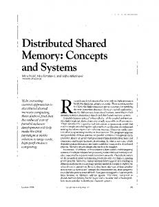
400 Exposure B, 70 mph Exposure B, 80 mph Exposure C, 70 mph Exposure C, 80 mph

350

Height Above Grade (ft)

300 250 200 150 100 50 0

0

5

10

15 20 25 30 35 40 Approximate Design Wind Pressure (psf)

45

50

Figure 2.7: Approximate Design Wind Pressure p for Ordinary Wind Force Resisting Building Structures

Example 2-2: Wind Load Determine the wind forces on the building shown on below which is built in St Louis and is surrounded by trees. Solution: 1. From Fig. 2.5 the maximum wind velocity is St. Louis is 70 mph, since the building is protected we can take Ce = 0.7, I = 1.. The base wind pressure is qs = 0.00256 × (70)2 = 12.54 psf.

Victor Saouma


Draft

2.3 Lateral Loads

41

Figure 2.8: Vibrations of a Building 36

The horizontal force at each level is calculated as a portion of the base shear force V V =

ZIC W RW

(2.8)

where: Z: Zone Factor: to be determined from Fig. 2.9 and Table 2.10.

Figure 2.9: Seismic Zones of the United States, (UBC 1995) I: Importance Factor: which was given by Table 2.8. Victor Saouma


Draft

2.3 Lateral Loads

Structural System

43

RW

Bearing wall system Light-framed walls with shear panels Plywood walls for structures three stories or less 8 All other light-framed walls 6 Shear walls Concrete 8 Masonry 8 Building frame system using trussing or shear walls) Steel eccentrically braced ductiel frame 10 Light-framed walls with shear panels Plywood walls for structures three stories or less 9 All other light-framed walls 7 Shear walls Concrete 8 Masonry 8 Concentrically braced frames Steel 8 Concrete (only for zones I and 2) 8 Heavy timber 8 Moment-resisting frame system Special moment-resisting frames (SMRF) Steel 12 Concrete 12 Concrete intermediate moment-resisting frames (IMRF)only for zones 1 and 2 8 Ordinary moment-resisting frames (OMRF) Steel 6 Concrete (only for zone 1) 5 Dual systems (selected cases are for ductile rigid frames only) Shear walls Concrete with SMRF 12 Masonry with SMRF 8 Steel eccentrically braced ductile frame 6-12 Concentrically braced frame 12 Steel with steel SMRF 10 Steel with steel OMRF 6 Concrete with concrete SMRF (only for zones 1 and 2) 9

H (ft)

65 65 240 160 240 65 65 240 160 160 65

N.L. N.L. 160 -

N.L. 160 160-N.L. N. L. N.L. 160 -

Table 2.12: Partial List of RW for Various Structure Systems, (UBC 1995)

Victor Saouma


Draft

2.3 Lateral Loads

45

5. The total vertical load is W = 2 ((200 + 0.5(400)) (20) = 16000 lbs

6. The total seismic base shear is ZIC (0.3)(1.25)(2.75) V = = = 0.086W RW 12 = (0.086)(16000) = 1375 lbs

(2.17)

(2.18-a) (2.18-b)

7. Since T < 0.7 sec. there is no whiplash. 8. The load on each floor is thus given by F2 = F1 =

(1375)(24) = 916.7 lbs 12 + 24 (1375)(12) = 458.3 lbs 12 + 24

(2.19-a) (2.19-b)

Example 2-4: Earthquake Load on a Tall Building, (Schueller 1996) Determine the approximate critical lateral loading for a 25 storey, ductile, rigid space frame concrete structure in the short direction. The rigid frames are spaced 25 ft apart in the cross section and 20 ft in the longitudinal direction. The plan dimension of the building is 175x100 ft, and the structure is 25(12)=300 ft high. This office building is located in an urban environment with a wind velocity of 70 mph and in seismic zone 4. For this investigation, an average building total dead load of 192 psf is used. Soil conditions are unknown. 470 k

25(12)=300’

2638 k

2(300)/3=200’

300/2=150’

1523 k

7(25)=175’

84000 k

3108 k

5(20)=100’

Victor Saouma


Draft

2.4 Other Loads

2.4

2.4.1 39

47

Other Loads Hydrostatic and Earth

Structures below ground must resist lateral earth pressure. (2.28)

q = Kγh where γ is the soil density, K = 40

1−sin Φ 1+sin Φ

is the pressure coefficient, h is the height.

For sand and gravel γ = 120 lb/ ft3 , and Φ ≈ 30◦ .

41 If the structure is partially submerged, it must also resist hydrostatic pressure of water, Fig. 2.10.

Figure 2.10: Earth and Hydrostatic Loads on Structures (2.29)

q = γW h where γW = 62.4 lbs/ft3 .

Example 2-5: Hydrostatic Load The basement of a building is 12 ft below grade. Ground water is located 9 ft below grade, what thickness concrete slab is required to exactly balance the hydrostatic uplift? Solution: The hydrostatic pressure must be countered by the pressure caused by the weight of concrete. Since p = γh we equate the two pressures and solve for h the height of the concrete slab (62.4) lbs/ft3 × (12 − 9) ft = (150) lbs/ft3 × h ⇒ h =

|

15.0 inch

{z

water

Victor Saouma

}

|

{z

concrete

}

3

(62.4) lbs/ft 3 (150) lbs/ft

(3) ft(12) in/ft = 14.976 in '


Draft

2.5 Other Important Considerations

2.4.3

49

Bridge Loads

For highway bridges, design loads are given by the AASHTO (Association of American State Highway Transportation Officials). The HS-20 truck is used for the design of bridges on main highways, Fig. 6.3. Either the design truck with specified axle loads and spacing must be used or the equivalent uniform load and concentrated load. This loading must be placed such that maximum stresses are produced.

Figure 2.11: Truck Load

2.4.4

2.5 2.5.1 45

Impact Load

Other Important Considerations Load Combinations

Live loads specified by codes represent the maximum possible loads.

The likelihood of all these loads occurring simultaneously is remote. Hence, building codes allow certain reduction when certain loads are combined together. 46

47

Furthermore, structures should be designed to resist a combination of loads.

Denoting D= dead; L= live; Lr= roof live; W= wind; E= earthquake; S= snow; T= temperature; H= soil: 48

49 For the load and resistance factor design (LRFD) method of concrete structures, the American Concrete Institute (ACI) Building design code (318) (318 n.d.) requires that the following load combinations be considered:

1. 1.4D+1.7L

Victor Saouma


Draft


51

Figure 2.12: Load Placement to Maximize Moments

Figure 2.13: Load Life of a Structure, (Lin and Stotesbury 1981)

Victor Saouma


Draft


53

1. The section is part of a beam or girder.

2. The beam or girder is really part of a three dimensional structure in which load is transmitted from any point in the structure to the foundation through any one of various structural forms. Load transfer in a structure is accomplished through a “hierarchy” of simple flexural elements which are then connected to the columns, Fig. 2.16 or by two way slabs as illustrated in Fig. 2.17.

57

58

An example of load transfer mechanism is shown in Fig. 2.18.

Victor Saouma


Draft


55

Figure 2.17: Two Way Actions

Victor Saouma


Draft Chapter 3

STRUCTURAL MATERIALS Proper understanding of structural materials is essential to both structural analysis and to structural design. 1

2

Characteristics of the most commonly used structural materials will be highlighted.

3.1 3.1.1

Steel Structural Steel

Steel is an alloy of iron and carbon. Its properties can be greatly varied by altering the carbon content (always less than 0.5%) or by adding other elements such as silicon, nickle, manganese and copper. 3

Practically all grades of steel have a Young Modulus equal to 29,000 ksi, density of 490 lb/cu ft, and a coefficient of thermal expansion equal to 0.65 × 10−5 /deg F.

4

The yield stress of steel can vary from 40 ksi to 250 ksi. Most commonly used structural steel are A36 (σyld = 36 ksi) and A572 (σyld = 50 ksi), Fig. 3.1

5

Structural steel can be rolled into a wide variety of shapes and sizes. Usually the most desirable members are those which have a large section moduli (S) in proportion to their area (A), Fig. 3.2. 6

7

Steel can be bolted, riveted or welded.

8 Sections are designated by the shape of their cross section, their depth and their weight. For example W 27× 114 is a W section, 27 in. deep weighing 114 lb/ft. 9

Common sections are:

S sections were the first ones rolled in America and have a slope on their inside flange surfaces of 1 to 6. W or wide flange sections have a much smaller inner slope which facilitates connections and rivetting. W sections constitute about 50% of the tonnage of rolled structural steel. C are channel sections MC Miscellaneous channel which can not be classified as a C shape by dimensions.

Draft 3.1 Steel

59

HP is a bearing pile section.

M is a miscellaneous section. L are angle sections which may have equal or unequal sides. WT is a T section cut from a W section in two. 10

The section modulus Sx of a W section can be roughly approximated by the following formula Sx ≈ wd/10 or Ix ≈ Sx

d ≈ wd2 /20 2

(3.1)

and the plastic modulus can be approximated by (3.2)

Zx ≈ wd/9 11

Properties of structural steel are tabulated in Table 3.1. ASTM Desig. A36

Shapes Available Shapes and bars

A500

Cold formed welded and seamless sections;

A501

Hot formed welded and seamless sections; Plates and bars 12 in and less thick;

A529

A606

Hot and cold rolled sheets;

A611

Cold rolled sheet in cut lengths Structural shapes, plates and bars

A 709

Use Riveted, bolted, welded; Buildings and bridges General structural purpose Riveted, welded or bolted; Bolted and welded Building frames and trusses; Bolted and welded Atmospheric corrosion resistant Cold formed sections Bridges

σy (kksi) 36 up through 8 in. above 8.)

σu (kksi) (32

Grade A: 33; Grade B: 42; Grade C: 46 36 42

45-50 Grade C 33; Grade D 40; Grade E 80 Grade 36: 36 (to 4 in.); Grade 50: 50; Grade 100: 100 (to 2.5in.) and 90 (over 2.5 to 4 in.)

Table 3.1: Properties of Major Structural Steels 12 Rolled sections, Fig. 3.3 and welded ones, Fig3.4 have residual stresses. Those originate during the rolling or fabrication of a member. The member is hot just after rolling or welding, it cools unevenly because of varying exposure. The area that cool first become stiffer, resist contraction, and develop compressive stresses. The remaining regions continue to cool and contract in the plastic condition and develop tensile stresses.

Due to those residual stresses, the stress-strain curve of a rolled section exhibits a non-linear segment prior to the theoretical yielding, Fig. 3.5. This would have important implications on the flexural and axial strength of beams and columns. 13

Victor Saouma


Draft

3.2 Aluminum

3.1.2

61

Reinforcing Steel

Steel is also used as reinforcing bars in concrete, Table 3.2. Those bars have a deformation on their surface to increase the bond with concrete, and usually have a yield stress of 60 ksi 1 .

14

Bar Designation No. 2 No. 3 No. 4 No. 5 No. 6 No. 7 No. 8 No. 9 No. 10 No. 11 No. 14 No. 18

Diameter (in.) 2/8=0.250 3/8=0.375 4/8=0.500 5/8=0.625 6/8=0.750 7/8=0.875 8/8=1.000 9/8=1.128 10/8=1.270 11/8=1.410 14/8=1.693 18/8=2.257

Area ( in2 ) 0.05 0.11 0.20 0.31 0.44 0.60 0.79 1.00 1.27 1.56 2.25 4.00

Perimeter in 0.79 1.18 1.57 1.96 2.36 2.75 3.14 3.54 3.99 4.43 5.32 7.09

Weight lb/ft 0.167 0.376 0.668 1.043 1.5202 2.044 2.670 3.400 4.303 5.313 7.650 13.60

Table 3.2: Properties of Reinforcing Bars Steel loses its strength rapidly above 700 deg. F (and thus must be properly protected from fire), and becomes brittle at −30 deg. F 15

Steel is also used as wire strands and ropes for suspended roofs, cable-stayed bridges, fabric roofs and other structural applications. A strand is a helical arrangement of wires around a central wire. A rope consists of multiple strands helically wound around a central plastic core, and a modulus of elasticity of 20,000 ksi, and an ultimate strength of 220 ksi.

16

17

Prestressing Steel cables have an ultimate strength up to 270 ksi.

3.2

Aluminum

18 Aluminum is used whenever light weight combined with strength is an important factor. Those properties, along with its resistance to corrosion have made it the material of choice for airplane structures, light roof framing. 19

Aluminum members can be connected by riveting, bolting and to a lesser extent by welding.

Aluminum has a modulus of elasticity equal to 10,000 ksi (about three times lower than steel), a coefficient of thermal expansion of 2.4 × 10−5 and a density of 173 lbs/ft3 .

20

21 The ultimate strength of pure aluminum is low (13,000 psi) but with the addition of alloys it can go up. 1

Stirrups which are used as vertical reinforcement to resist shear usually have a yield stress of only 40 ksi.

Victor Saouma


Draft 3.4 Masonry

63

30

Density of normal weight concrete is 145 lbs/ft3 and 100 lbs/ft3 for lightweight concrete.

31

Coefficient of thermal expansion is 0.65 × 10−5 /deg F for normal weight concrete.

When concrete is poured (or rather placed), the free water not needed for the hydration process evaporates over a period of time and the concrete will shrink. This shrinkage is about 0.05% after one year (strain). Thus if the concrete is restrained, then cracking will occur 3 . 32

Concrete will also deform with time due to the applied load, this is called creep. This should be taken into consideration when computing the deflections (which can be up to three times the instantaneous elastic deflection). 33

3.4

Masonry

Masonry consists of either natural materials, such as stones, or of manufactured products such as bricks and concrete blocks4 , stacked and bonded together with mortar.

34

As for concrete, all modern structural masonry blocks are essentially compression members with low tensile resistance. 35

The mortar used is a mixture of sand, masonry cement, and either Portland cement or hydrated lime.

36

3.5

Timber

37 Timber is one of the earliest construction materials, and one of the few natural materials with good tensile properties. 38

The properties of timber vary greatly, and the strength is time dependent.

Timber is a good shock absorber (many wood structures in Japan have resisted repeated earthquakes). 39

40 The most commonly used species of timber in construction are Douglas fir, southern pine, hemlock and larch.

Members can be laminated together under good quality control, and flexural strengths as high as 2,500 psi can be achieved.

41

3.6 42

Steel Section Properties

Dimensions and properties of rolled sections are tabulated in the following pages, Fig. 3.7. ==============

3 For this reason a minimum amount of reinforcement is always necessary in concrete, and a 2% reinforcement, can reduce the shrinkage by 75%. 4 Mud bricks were used by the Babylonians, stones by the Egyptians, and ice blocks by the Eskimos...

Victor Saouma


Draft

3.6 Steel Section Properties Designation

A in2 W 27x539 158.0 W 27x494 145.0 W 27x448 131.0 W 27x407 119.0 W 27x368 108.0 W 27x336 98.7 W 27x307 90.2 W 27x281 82.6 W 27x258 75.7 W 27x235 69.1 W 27x217 63.8 W 27x194 57.0 W 27x178 52.3 W 27x161 47.4 W 27x146 42.9 W 27x129 37.8 W 27x114 33.5 W 27x102 30.0 W 27x 94 27.7 W 27x 84 24.8 W 24x492 144.0 W 24x450 132.0 W 24x408 119.0 W 24x370 108.0 W 24x335 98.4 W 24x306 89.8 W 24x279 82.0 W 24x250 73.5 W 24x229 67.2 W 24x207 60.7 W 24x192 56.3 W 24x176 51.7 W 24x162 47.7 W 24x146 43.0 W 24x131 38.5 W 24x117 34.4 W 24x104 30.6 W 24x103 30.3 W 24x 94 27.7 W 24x 84 24.7 W 24x 76 22.4 W 24x 68 20.1 W 24x 62 18.2 W 24x 55 16.2 W 21x402 118.0 W 21x364 107.0 W 21x333 97.9 W 21x300 88.2 W 21x275 80.8 W 21x248 72.8 W 21x223 65.4 W 21x201 59.2 W 21x182 53.6 W 21x166 48.8 W 21x147 43.2 W 21x132 38.8 W 21x122 35.9 W 21x111 32.7 W 21x101 Victor Saouma 29.8 W 21x 93 27.3 W 21x 83 24.3 W 21x 73 21.5

d in 32.52 31.97 31.42 30.87 30.39 30.00 29.61 29.29 28.98 28.66 28.43 28.11 27.81 27.59 27.38 27.63 27.29 27.09 26.92 26.71 29.65 29.09 28.54 27.99 27.52 27.13 26.73 26.34 26.02 25.71 25.47 25.24 25.00 24.74 24.48 24.26 24.06 24.53 24.31 24.10 23.92 23.73 23.74 23.57 26.02 25.47 25.00 24.53 24.13 23.74 23.35 23.03 22.72 22.48 22.06 21.83 21.68 21.51 21.36 21.62 21.43 21.24

bf 2tf

2.2 2.3 2.5 2.7 3.0 3.2 3.5 3.7 4.0 4.4 4.7 5.2 5.9 6.5 7.2 4.5 5.4 6.0 6.7 7.8 2.0 2.1 2.3 2.5 2.7 2.9 3.2 3.5 3.8 4.1 4.4 4.8 5.3 5.9 6.7 7.5 8.5 4.6 5.2 5.9 6.6 7.7 6.0 6.9 2.1 2.3 2.5 2.7 2.9 3.2 3.5 3.9 4.2 4.6 5.4 6.0 6.5 7.1 7.7 4.5 5.0 5.6

65 hc tw

Ix Sx Iy Sy in4 in3 in4 in3 12.3 25500 1570 2110 277 13.4 22900 1440 1890 250 14.7 20400 1300 1670 224 15.9 18100 1170 1480 200 17.6 16100 1060 1310 179 19.2 14500 970 1170 161 20.9 13100 884 1050 146 22.9 11900 811 953 133 24.7 10800 742 859 120 26.6 9660 674 768 108 29.2 8870 624 704 100 32.3 7820 556 618 88 33.4 6990 502 555 79 36.7 6280 455 497 71 40.0 5630 411 443 64 39.7 4760 345 184 37 42.5 4090 299 159 32 47.0 3620 267 139 28 49.4 3270 243 124 25 52.7 2850 213 106 21 10.9 19100 1290 1670 237 11.9 17100 1170 1490 214 13.1 15100 1060 1320 191 14.2 13400 957 1160 170 15.6 11900 864 1030 152 17.1 10700 789 919 137 18.6 9600 718 823 124 20.7 8490 644 724 110 22.5 7650 588 651 99 24.8 6820 531 578 89 26.6 6260 491 530 82 28.7 5680 450 479 74 30.6 5170 414 443 68 33.2 4580 371 391 60 35.6 4020 329 340 53 39.2 3540 291 297 46 43.1 3100 258 259 41 39.2 3000 245 119 26 41.9 2700 222 109 24 45.9 2370 196 94 21 49.0 2100 176 82 18 52.0 1830 154 70 16 50.1 1550 131 34 10 54.6 1350 114 29 8 10.8 12200 937 1270 189 11.8 10800 846 1120 168 12.8 9610 769 994 151 14.2 8480 692 873 134 15.4 7620 632 785 122 17.1 6760 569 694 109 18.8 5950 510 609 96 20.6 5310 461 542 86 22.6 4730 417 483 77 24.9 4280 380 435 70 26.1 3630 329 376 60 28.9 3220 295 333 54 31.3 2960 273 305 49 34.1 2670 249 274 44 37.5 2420 227 248 40 Structural Concepts and 32.3 2070 192 93 22 36.4 1830 171 81 20 41.2 1600 151 71 17

Zx Zy in3 in3 1880.0 437.0 1710.0 394.0 1530.0 351.0 1380.0 313.0 1240.0 279.0 1130.0 252.0 1020.0 227.0 933.0 206.0 850.0 187.0 769.0 168.0 708.0 154.0 628.0 136.0 567.0 122.0 512.0 109.0 461.0 97.5 395.0 57.6 343.0 49.3 305.0 43.4 278.0 38.8 244.0 33.2 1550.0 375.0 1410.0 337.0 1250.0 300.0 1120.0 267.0 1020.0 238.0 922.0 214.0 835.0 193.0 744.0 171.0 676.0 154.0 606.0 137.0 559.0 126.0 511.0 115.0 468.0 105.0 418.0 93.2 370.0 81.5 327.0 71.4 289.0 62.4 280.0 41.5 254.0 37.5 224.0 32.6 200.0 28.6 177.0 24.5 153.0 15.7 134.0 13.3 1130.0 296.0 1010.0 263.0 915.0 237.0 816.0 210.0 741.0 189.0 663.0 169.0 589.0 149.0 530.0 133.0 476.0 119.0 432.0 108.0 373.0 92.6 333.0 82.3 307.0 75.6 279.0 68.2 253.0 Systems61.7 for 221.0 34.7 196.0 30.5 172.0 26.6

Architects

Draft


W 14x 74 W 14x 68 W 14x 61 W 14x 53 W 14x 48 W 14x 43 W 14x 38 W 14x 34 W 14x 30 W 14x 26 W 14x 22 W 12x336 W 12x305 W 12x279 W 12x252 W 12x230 W 12x210 W 12x190 W 12x170 W 12x152 W 12x136 W 12x120 W 12x106 W 12x 96 W 12x 87 W 12x 79 W 12x 72 W 12x 65 W 12x 58 W 12x 53 W 12x 50 W 12x 45 W 12x 40 W 12x 35 W 12x 30 W 12x 26 W 12x 22 W 12x 19 W 12x 16 W 12x 14 W 10x112 W 10x100 W 10x 88 W 10x 77 W 10x 68 W 10x 60 W 10x 54 W 10x 49 W 10x 45 W 10x 39 W 10x 33 W 10x 30 W 10x 26 W 10x 22 W 10x 19 W 10x 17 W 10x 15 W 10x 12

Victor Saouma

A in2 21.8 20.0 17.9 15.6 14.1 12.6 11.2 10.0 8.9 7.7 6.5 98.8 89.6 81.9 74.1 67.7 61.8 55.8 50.0 44.7 39.9 35.3 31.2 28.2 25.6 23.2 21.1 19.1 17.0 15.6 14.7 13.2 11.8 10.3 8.8 7.7 6.5 5.6 4.7 4.2 32.9 29.4 25.9 22.6 20.0 17.6 15.8 14.4 13.3 11.5 9.7 8.8 7.6 6.5 5.6 5.0 4.4 3.5

d in 14.17 14.04 13.89 13.92 13.79 13.66 14.10 13.98 13.84 13.91 13.74 16.82 16.32 15.85 15.41 15.05 14.71 14.38 14.03 13.71 13.41 13.12 12.89 12.71 12.53 12.38 12.25 12.12 12.19 12.06 12.19 12.06 11.94 12.50 12.34 12.22 12.31 12.16 11.99 11.91 11.36 11.10 10.84 10.60 10.40 10.22 10.09 9.98 10.10 9.92 9.73 10.47 10.33 10.17 10.24 10.11 9.99 9.87

bf 2tf

6.4 7.0 7.7 6.1 6.7 7.5 6.6 7.4 8.7 6.0 7.5 2.3 2.4 2.7 2.9 3.1 3.4 3.7 4.0 4.5 5.0 5.6 6.2 6.8 7.5 8.2 9.0 9.9 7.8 8.7 6.3 7.0 7.8 6.3 7.4 8.5 4.7 5.7 7.5 8.8 4.2 4.6 5.2 5.9 6.6 7.4 8.2 8.9 6.5 7.5 9.1 5.7 6.6 8.0 5.1 6.1 7.4 9.4

67 hc tw

25.3 27.5 30.4 30.8 33.5 37.4 39.6 43.1 45.4 48.1 53.3 5.5 6.0 6.3 7.0 7.6 8.2 9.2 10.1 11.2 12.3 13.7 15.9 17.7 18.9 20.7 22.6 24.9 27.0 28.1 26.2 29.0 32.9 36.2 41.8 47.2 41.8 46.2 49.4 54.3 10.4 11.6 13.0 14.8 16.7 18.7 21.2 23.1 22.5 25.0 27.1 29.5 34.0 36.9 35.4 36.9 38.5 46.6

Ix in4 796 723 640 541 485 428 385 340 291 245 199 4060 3550 3110 2720 2420 2140 1890 1650 1430 1240 1070 933 833 740 662 597 533 475 425 394 350 310 285 238 204 156 130 103 89 716 623 534 455 394 341 303 272 248 209 170 170 144 118 96 82 69 54

Sx in3 112 103 92 78 70 63 55 49 42 35 29 483 435 393 353 321 292 263 235 209 186 163 145 131 118 107 97 88 78 71 65 58 52 46 39 33 25 21 17 15 126 112 98 86 76 67 60 55 49 42 35 32 28 23 19 16 14 11

Iy in4 134 121 107 58 51 45 27 23 20 9 7 1190 1050 937 828 742 664 589 517 454 398 345 301 270 241 216 195 174 107 96 56 50 44 24 20 17 5 4 3 2 236 207 179 154 134 116 103 93 53 45 37 17 14 11 4 4 3 2

Sy in3 27 24 22 14 13 11 8 7 6 4 3 177 159 143 127 115 104 93 82 73 64 56 49 44 40 36 32 29 21 19 14 12 11 7 6 5 2 2 1 1 45 40 35 30 26 23 21 19 13 11 9 6 5 4 2 2 1 1

Zx in3 126.0 115.0 102.0 87.1 78.4 69.6 61.5 54.6 47.3 40.2 33.2 603.0 537.0 481.0 428.0 386.0 348.0 311.0 275.0 243.0 214.0 186.0 164.0 147.0 132.0 119.0 108.0 96.8 86.4 77.9 72.4 64.7 57.5 51.2 43.1 37.2 29.3 24.7 20.1 17.4 147.0 130.0 113.0 97.6 85.3 74.6 66.6 60.4 54.9 46.8 38.8 36.6 31.3 26.0 21.6 18.7 16.0 12.6

Zy in3 40.6 36.9 32.8 22.0 19.6 17.3 12.1 10.6 9.0 5.5 4.4 274.0 244.0 220.0 196.0 177.0 159.0 143.0 126.0 111.0 98.0 85.4 75.1 67.5 60.4 54.3 49.2 44.1 32.5 29.1 21.4 19.0 16.8 11.5 9.6 8.2 3.7 3.0 2.3 1.9 69.2 61.0 53.1 45.9 40.1 35.0 31.3 28.3 20.3 17.2 14.0 8.8 7.5 6.1 3.3 2.8 2.3 1.7


Draft


C 15.x 50 C 15.x 40 C 15.x 34 C 12.x 30 C 12.x 25 C 12.x 21 C 10.x 30 C 10.x 25 C 10.x 20 C 10.x 15 C 9.x 20 C 9.x 15 C 9.x 13 C 8.x 19 C 8.x 14 C 8.x 12 C 7.x 15 C 7.x 12 C 7.x 10 C 6.x 13 C 6.x 11 C 6.x 8 C 5.x 9 C 5.x 7 C 4.x 7 C 4.x 5 C 3.x 6 C 3.x 5 C 3.x 4

Victor Saouma

A in2 14.7 11.8 10.0 8.8 7.3 6.1 8.8 7.3 5.9 4.5 5.9 4.4 3.9 5.5 4.0 3.4 4.3 3.6 2.9 3.8 3.1 2.4 2.6 2.0 2.1 1.6 1.8 1.5 1.2

d in 15. 15. 15. 12. 12. 12. 10. 10. 10. 10. 9. 9. 9. 8. 8. 8. 7. 7. 7. 6. 6. 6. 5. 5. 4. 4. 3. 3. 3.

bf 2tf

0 0 0 0 0 0 0 0 0 0 0 0 0 0 0 0 0 0 0 0 0 0 0 0 0 0 0 0 0

69 hc tw

0 0 0 0 0 0 0 0 0 0 0 0 0 0 0 0 0 0 0 0 0 0 0 0 0 0 0 0 0

Ix in4 404.0 349.0 315.0 162.0 144.0 129.0 103.0 91.2 78.9 67.4 60.9 51.0 47.9 44.0 36.1 32.6 27.2 24.2 21.3 17.4 15.2 13.1 8.9 7.5 4.6 3.8 2.1 1.9 1.7

Sx in3 53.8 46.5 42.0 27.0 24.1 21.5 20.7 18.2 15.8 13.5 13.5 11.3 10.6 11.0 9.0 8.1 7.8 6.9 6.1 5.8 5.1 4.4 3.6 3.0 2.3 1.9 1.4 1.2 1.1

Iy in4 11. 9.23 8.13 5.14 4.47 3.88 3.94 3.36 2.81 2.28 2.42 1.93 1.76 1.98 1.53 1.32 1.38 1.17 0.97 1.05 0.87 0.69 0.63 0.48 0.43 0.32 0.31 0.25 0.20

Sy in3 3.78 3.37 3.11 2.06 1.88 1.73 1.65 1.48 1.32 1.16 1.17 1.01 0.96 1.01 0.85 0.78 0.78 0.70 0.63 0.64 0.56 0.49 0.45 0.38 0.34 0.28 0.27 0.23 0.20

Zx in3 8.20 57.20 50.40 33.60 29.20 25.40 26.60 23. 19.30 15.80 16.80 13.50 12.50 13.80 10.90 9.55 9.68 8.40 7.12 7.26 6.15 5.13 4.36 3.51 2.81 2.26 1.72 1.50 1.30

Zy in3 8.17 6.87 6.23 4.33 3.84 3.49 3.78 3.19 2.71 2.35 2.47 2.05 1.95 2.17 1.73 1.58 1.64 1.43 1.26 1.36 1.15 0.99 0.92 0.76 0.70 0.57 0.54 0.47 0.40


Draft


L L L L L L L L L L L L L L L L L L L L L L L L L L L L L L L L L L

5.0x5.0x0.875 5.0x5.0x0.750 5.0x5.0x0.625 5.0x5.0x0.500 5.0x5.0x0.438 5.0x5.0x0.375 5.0x5.0x0.313 5.0x3.5x0.750 5.0x3.5x0.625 5.0x3.5x0.500 5.0x3.5x0.438 5.0x3.5x0.375 5.0x3.5x0.313 5.0x3.5x0.250 5.0x3.0x0.625 5.0x3.0x0.500 5.0x3.0x0.438 5.0x3.0x0.375 5.0x3.0x0.313 5.0x3.0x0.250 4.0x4.0x0.750 4.0x4.0x0.625 4.0x4.0x0.500 4.0x4.0x0.438 4.0x4.0x0.375 4.0x4.0x0.313 4.0x4.0x0.250 4.0x3.5x0.500 4.0x3.5x0.438 4.0x3.5x0.375 4.0x3.5x0.313 4.0x3.5x0.250 4.0x3.0x0.500 4.0x3.0x0.438

Victor Saouma

A in2 7.98 6.94 5.86 4.75 4.18 3.61 3.03 5.81 4.92 4.00 3.53 3.05 2.56 2.06 4.61 3.75 3.31 2.86 2.40 1.94 5.44 4.61 3.75 3.31 2.86 2.40 1.94 3.50 3.09 2.67 2.25 1.81 3.25 2.87

wgt k/f t 27.20 23.60 20.00 16.20 14.30 12.30 10.30 19.80 16.80 13.60 12.00 10.40 8.70 7.00 15.70 12.80 11.30 9.80 8.20 6.60 18.50 15.70 12.80 11.30 9.80 8.20 6.60 11.90 10.60 9.10 7.70 6.20 11.10 9.80

71 Ix in4 17.8 15.7 13.6 11.3 10.0 8.7 7.4 13.9 12.0 10.0 8.9 7.8 6.6 5.4 11.4 9.4 8.4 7.4 6.3 5.1 7.7 6.7 5.6 5.0 4.4 3.7 3.0 5.3 4.8 4.2 3.6 2.9 5.1 4.5

Sx in3 5.2 4.5 3.9 3.2 2.8 2.4 2.0 4.3 3.7 3.0 2.6 2.3 1.9 1.6 3.5 2.9 2.6 2.2 1.9 1.5 2.8 2.4 2.0 1.8 1.5 1.3 1.0 1.9 1.7 1.5 1.3 1.0 1.9 1.7

Iy in4 17.80 15.70 13.60 11.30 10.00 8.74 7.42 5.55 4.83 4.05 3.63 3.18 2.72 2.23 3.06 2.58 2.32 2.04 1.75 1.44 7.67 6.66 5.56 4.97 4.36 3.71 3.04 3.79 3.40 2.95 2.55 2.09 2.42 2.18

Sy in3 5.17 4.53 3.86 3.16 2.79 2.42 2.04 2.22 1.90 1.56 1.39 1.21 1.02 0.83 1.39 1.15 1.02 0.89 0.75 0.61 2.81 2.40 1.97 1.75 1.52 1.29 1.05 1.52 1.35 1.16 0.99 0.81 1.12 0.99

Zx in3 9.33 8.16 6.95 5.68 5.03 4.36 3.68 7.65 6.55 5.38 4.77 4.14 3.49 2.83 6.27 5.16 4.57 3.97 3.36 2.72 5.07 4.33 3.56 3.16 2.74 2.32 1.88 3.50 3.11 2.71 2.29 1.86 3.41 3.03

Zy in3 9.33 8.16 6.95 5.68 5.03 4.36 3.68 4.10 3.47 2.83 2.49 2.16 1.82 1.47 2.61 2.11 1.86 1.60 1.35 1.09 5.07 4.33 3.56 3.16 2.74 2.32 1.88 2.73 2.42 2.11 1.78 1.44 2.03 1.79


Draft 3.7 Joists

3.7

73

Joists

43 Steel joists, Fig. 3.8 look like shallow trusses (warren type) and are designed as simply supported uniformly loaded beams assuming that they are laterally supported on the top (to prevent lateral torsional buckling). The lateral support is often profided by the concrete slab it suppors.

The standard open-web joist designation consists of the depth, the series designation and the chord type. Three series are available for floor/roof construction, Table 3.3

44

Series K LH DLH

Depth (in) 8-30 18-48 52-72

Span (ft) 8-60 25-96 89-120

Table 3.3: Joist Series Characteristics [Design Length = Span – 0.33 FT.]

4"

4" 4"

Span Figure 3.8: prefabricated Steel Joists 45 Typical joist spacing ranges from 2 to 4 ft, and provides an efficient use of the corrugated steel deck which itself supports the concrete slab. 46 For preliminary estimates of the joist depth, a depth to span ratio of 24 can be assumed, therefore

d ≈ L/2

(3.5)

where d is in inches, and L in ft. Table 3.4 list the load carrying capacity of open web, K-series steel joists based on a amximum allowable stress of 30 ksi. For each span, the first line indicates the total safe uniformly 47

Victor Saouma


Draft 3.7 Joists

75

Joint 8K1 10K1 12K1 12K3 12K5 Desig. Depth 8 10 12 12 12 (in.) ≈ 5.1 5 5 5.7 7.1 W (lbs/ft) Span (ft.) 8 550 550 9 550 550 10 550 550 480 550 11 532 550 377 542 12 444 550 550 550 550 288 455 550 550 550 13 377 479 550 550 550 225 363 510 510 510 14 324 412 500 550 550 179 289 425 463 463 15 281 358 434 543 550 145 234 344 428 434 16 246 313 380 476 550 119 192 282 351 396 17 277 336 420 550 159 234 291 366 18 246 299 374 507 134 197 245 317 19 221 268 335 454 113 167 207 269 20 199 241 302 409 97 142 177 230 21 218 273 370 123 153 198 22 199 249 337 106 132 172 23 181 227 308 93 116 150 24 166 208 282 81 101 132 25 26 27 28 29 30 31 32

Victor Saouma

14K1 14K3 14K4 14K6 16K2 16K3 16K4 16K5 16K6 16K7 16K9 14

14

14

14

16

16

16

16

16

16

16

5.2

6

6.7

7.7

5.5

6.3

7

7.5

8.1

8.6

10.0

550 550 511 475 448 390 395 324 352 272 315 230 284 197 257 170 234 147 214 128 196 113 180 100 166 88 154 79 143 70

550 550 550 507 550 467 495 404 441 339 395 287 356 246 322 212 293 184 268 160 245 141 226 124 209 110 193 98 180 88

550 550 550 507 550 467 550 443 530 397 475 336 428 287 388 248 353 215 322 188 295 165 272 145 251 129 233 115 216 103

550 550 550 507 550 467 550 443 550 408 550 383 525 347 475 299 432 259 395 226 362 199 334 175 308 56 285 139 265 124

550 550 512 488 456 409 408 347 368 297 333 255 303 222 277 194 254 170 234 150 216 133 200 119 186 106 173 95 161 86 151 78 142 71

550 550 550 526 508 456 455 386 410 330 371 285 337 247 308 216 283 189 260 167 240 148 223 132 207 118 193 106 180 96 168 87 158 79

550 550 550 526 550 490 547 452 493 386 447 333 406 289 371 252 340 221 313 195 289 173 268 155 249 138 232 124 216 112 203 101 190 92

550 550 550 526 550 490 550 455 550 426 503 373 458 323 418 282 384 248 353 219 326 194 302 173 281 155 261 139 244 126 228 114 214 103

550 550 550 526 550 490 550 455 550 426 548 405 498 351 455 307 418 269 384 238 355 211 329 188 306 168 285 151 266 137 249 124 233 112

550 550 550 526 550 490 550 455 550 426 550 406 550 385 507 339 465 298 428 263 395 233 366 208 340 186 317 167 296 151 277 137 259 124

550 550 550 526 550 490 550 455 550 426 550 406 550 385 550 363 550 346 514 311 474 276 439 246 408 220 380 198 355 178 332 161 311 147

Structural Concepts and Systems for Architects Table 3.4: Joist Properties

Draft Chapter 4

Case Study I: EIFFEL TOWER Adapted from (Billington and Mark 1983)

4.1

Materials, & Geometry

1 The tower was built out of wrought iron, less expensive than steel,and Eiffel had more expereince with this material, Fig. 4.1

Figure 4.1: Eiffel Tower (Billington and Mark 1983)

Draft 4.2 Loads

79

Location Support First platform second platform Intermediate platform Top platform Top

Height 0 186 380 644 906 984

Width/2 164 108 62 20 1 0

Width Estimated Actual 328 216 240 123 110 40 2 0

dy dx

.333 .270 .205 .115 .0264 0.000

β 18.4o 15.1o 11.6o 6.6o 1.5o 0o

The tower is supported by four inclined supports, each with a cross section of 800 in 2 . An idealization of the tower is shown in Fig. 4.2. 4

ACTUAL CONTINUOUS CONNECTION

IDEALIZED CONTINUOUS CONNECTION

ACTUAL POINTS OF CONNECTION

Figure 4.2: Eiffel Tower Idealization, (Billington and Mark 1983)

4.2

Loads

5

The total weight of the tower is 18, 800 k.

6

The dead load is not uniformly distributed, and is approximated as follows, Fig. 4.3:

Figure 4.3: Eiffel Tower, Dead Load Idealization; (Billington and Mark 1983)

Victor Saouma


Draft

4.3 Reactions

81

LOADS

TOTAL LOADS

P

Q

P=2560k

V

Q=22,280k

L/2

H0 REACTIONS

0

M0

Figure 4.5: Eiffel Tower, Wind Loads, (Billington and Mark 1983)

+

=

WINDWARD SIDE

VERTICAL FORCES

WIND FORCES

LEEWARD SIDE

TOTAL

Figure 4.6: Eiffel Tower, Reactions; (Billington and Mark 1983)

Victor Saouma


Draft

4.4 Internal Forces

83

0

β=18.4

INCLINED INTERNAL FORCE: N CONSEQUENT HORIZONTAL COMPONENT: H

KNOWN VERTICAL COMPONENT: V

β=18.4 N

V

H FORCE POLYGON

Figure 4.7: Eiffel Tower, Internal Gravity Forces; (Billington and Mark 1983) 12 Gravity load are first considered, remember those are caused by the dead load and the live load, Fig. 4.7:

V V ⇒N = N cos β 11, 140 k N = = 11,730 kip cos 18.4o H tan β = ⇒ H = V tan β V H = 11, 140 k(tan 18.4o ) = 3,700 kip cos β =

(4.12-a) (4.12-b) (4.12-c) (4.12-d)

The horizontal forces which must be resisted by the foundations, Fig. 4.8.

H

H 3700 k

3700 k

Figure 4.8: Eiffel Tower, Horizontal Reactions; (Billington and Mark 1983) 13

Because the vertical load decreases with height, the axial force will also decrease with height.

14 At the second platform, the total vertical load is Q = 1, 100 + 2, 200 = 3, 300 k and at that height the angle is 11.6o thus the axial force (per pair of columns) will be

Nvert =

3,300 2

k

= 1, 685 k (4.13-a) cos 11.6o 3, 300 k (tan 11.6o ) = 339 k (4.13-b) Hvert = 2 Note that this is about seven times smaller than the axial force at the base, which for a given axial strength, would lead the designer to reduce (or taper) the cross-section. Victor Saouma


Draft Chapter 5

REVIEW of STATICS To every action there is an equal and opposite reaction. Newton’s third law of motion

5.1

Reactions

In the analysis of structures (hand calculations), it is often easier (but not always necessary) to start by determining the reactions.

1

Once the reactions are determined, internal forces are determined next; finally, internal stresses and/or deformations (deflections and rotations) are determined last 1 .

2

3

Reactions are necessary to determine foundation load.

Depending on the type of structures, there can be different types of support conditions, Fig. 5.1.

4

Roller: provides a restraint in only one direction in a 2D structure, in 3D structures a roller may provide restraint in one or two directions. A roller will allow rotation. Hinge: allows rotation but no displacements. Fixed Support: will prevent rotation and displacements in all directions.

5.1.1

Equilibrium

5

Reactions are determined from the appropriate equations of static equilibrium.

6

Summation of forces and moments, in a static system must be equal to zero2 . 1

This is the sequence of operations in the flexibility method which lends itself to hand calculation. In the stiffness method, we determine displacements firsts, then internal forces and reactions. This method is most suitable to computer implementation. 2 In a dynamic system ΣF = ma where m is the mass and a is the acceleration.

Draft

5.1 Reactions

87

Structure Type Beam, no axial forces 2D Truss, Frame, Beam Grid 3D Truss, Frame Beams, no axial Force 2 D Truss, Frame, Beam

Equations ΣFx

ΣFy ΣFy

ΣFz ΣFx ΣFy ΣFz Alternate Set ΣMzA ΣMzB ΣFx ΣMzA ΣMzB ΣMzA ΣMzB ΣMzC

ΣMz ΣMz ΣMx ΣMx

ΣMy ΣMy

ΣMz

Table 5.1: Equations of Equilibrium 2. Assume a direction for the unknown quantities 3. The right hand side of the equation should be zero If your reaction is negative, then it will be in a direction opposite from the one assumed. Summation of external forces is equal and opposite to the internal ones. Thus the net force/moment is equal to zero.

16

17

The external forces give rise to the (non-zero) shear and moment diagram.

5.1.2

Equations of Conditions

If a structure has an internal hinge (which may connect two or more substructures), then this will provide an additional equation (ΣM = 0 at the hinge) which can be exploited to determine the reactions.

18

Those equations are often exploited in trusses (where each connection is a hinge) to determine reactions. 19

In an inclined roller support with Sx and Sy horizontal and vertical projection, then the reaction R would have, Fig. 5.2.

20

Sy Rx = Ry Sx

(5.3)

Figure 5.2: Inclined Roller Support

Victor Saouma


Draft

5.1 Reactions

89

Figure 5.4: Geometric Instability Caused by Concurrent Reactions

5.1.5

Examples

Examples of reaction calculation will be shown next. Each example has been carefully selected as it brings a different “twist” from the preceding one. Some of those same problems will be revisited later for the determination of the internal forces and/or deflections. Many of those problems are taken from Prof. Gerstle textbok Basic Structural Analysis.

29

Example 5-1: Simply Supported Beam Determine the reactions of the simply supported beam shown below.

Solution: The beam has 3 reactions, we have 3 equations of static equilibrium, hence it is statically determinate. (+ - ) ΣFx = 0; ⇒ Rax − 36 k = 0 (+ 6) ΣFy = 0; ⇒ Ray + Rdy − 60 k − (4) k/ft(12) ft = 0 (+ ) ΣMzc = 0; ⇒ 12Ray − 6Rdy − (60)(6) = 0 or through matrix inversion (on your calculator) 

















  1 0 0  Rax     36    Rax     36 k     1  Ray 108 Ray 56 k = ⇒ =  0 1          0 12 −6  Rdy   360  Rdy   52 k 

Alternatively we could have used another set of equations:

(+ ) ΣMza = 0; (60)(6) + (48)(12) − (Rdy )(18) = 0 ⇒ Rdy = 52 k 6 (+ ) ΣMzd = 0; (Ray )(18) − (60)(12) − (48)(6) = 0 ⇒ Ray = 56 k 6 Victor Saouma


Draft

5.1 Reactions

91

2. Isolating bd: (+ ) ΣMd = 0; −(17.7)(18) − (40)(15) − (4)(8)(8) − (30)(2) + R cy (12) = 0 ⇒ Rcy = 1,236 12 = 103 k 6 (+ ) ΣMc = 0; −(17.7)(6) − (40)(3) + (4)(8)(4) + (30)(10) − R dy (12) = 0 ⇒ Rdy = 201.3 12 = 16.7 k 6 3. Check ΣFy = 0; 6; 22.2 − 40 − 40 + 103 − 32 − 30 + 16.7 = 0

√

Example 5-3: Three Hinged Gable Frame The three-hinged gable frames spaced at 30 ft. on center. Determine the reactions components on the frame due to: 1) Roof dead load, of 20 psf of roof area; 2) Snow load, of 30 psf of horizontal projection; 3) Wind load of 15 psf of vertical projection. Determine the critical design values for the vertical and horizontal reactions.

Solution: 1. Due to symmetry, we will consider only the dead load on one side of the frame. Victor Saouma


Draft 5.2 Trusses

5.2

5.2.1

93

Trusses Assumptions

Cables and trusses are 2D or 3D structures composed of an assemblage of simple one dimensional components which transfer only axial forces along their axis.

30

31

Trusses are extensively used for bridges, long span roofs, electric tower, space structures.

32

For trusses, it is assumed that 1. Bars are pin-connected 2. Joints are frictionless hinges4 . 3. Loads are applied at the joints only.

A truss would typically be composed of triangular elements with the bars on the upper chord under compression and those along the lower chord under tension. Depending on the orientation of the diagonals, they can be under either tension or compression.

33

In a truss analysis or design, we seek to determine the internal force along each member, Fig. 5.5

34

Figure 5.5: Bridge Truss

5.2.2

Basic Relations

Sign Convention: Tension positive, compression negative. On a truss the axial forces are indicated as forces acting on the joints. Stress-Force: σ =

P A

Stress-Strain: σ = Eε Force-Displacement: ε =

∆L L

4 In practice the bars are riveted, bolted, or welded directly to each other or to gusset plates, thus the bars are not free to rotate and so-called secondary bending moments are developed at the bars. Another source of secondary moments is the dead weight of the element.

Victor Saouma


Draft 5.2 Trusses

95

Figure 5.6: A Statically Indeterminate Truss 3. Sketch a free body diagram showing all joint loads (including reactions) 4. For each joint, and starting with the loaded ones, apply the appropriate equations of equilibrium (ΣFx and ΣFy in 2D; ΣFx , ΣFy and ΣFz in 3D). 5. Because truss elements can only carry axial forces, the resultant force ( F~ = F~x + F~y ) must be along the member, Fig. 5.7. F Fx Fy = = l lx ly

(5.4)

Always keep track of the x and y components of a member force (Fx , Fy ), as those might be needed later on when considering the force equilibrium at another joint to which the member is connected.

44

Figure 5.7: X and Y Components of Truss Forces

45

This method should be used when all member forces should be determined.

In truss analysis, there is no sign convention. A member is assumed to be under tension (or compression). If after analysis, the force is found to be negative, then this would imply that the wrong assumption was made, and that the member should have been under compression (or tension).

46

Victor Saouma


Draft 5.2 Trusses

97

Node A: Clearly AH is under compression, and AB under tension.

(+ 6) ΣFy = 0; ⇒ FAHy − 58 = 0 FAH = lly (FAHy ) √ ly = 32 l = 322 + 242 = 40 Compression ⇒ FAH = 40 32 (58) = 72.5 (+ ) ΣFx = 0; ⇒ −FAHx + FAB = 0 FAB = llxy (FAHy ) = 24 32 (58) = 43.5 Tension Node B:

(+ - ) ΣFx = 0; ⇒ FBC (+ 6) ΣFy = 0; ⇒ FBH

= 43.5 Tension = 20 Tension

Node H:

(+ - ) ΣFx = 0; ⇒ FAHx − FHCx − FHGx = 0 43.5 − √2424 (FHC ) − √2424 (FHG ) = 0 (I) 2 +322 2 +102 (+ 6) ΣFy = 0; ⇒ FAHy + FHCy − 12 − FHGy − 20 = 0 58 + √2432 (FHC ) − 12 − √2410 (FHG ) − 20 = 0 (II) 2 +322 2 +102 Solving for I and II we obtain FHC = −7.5 Tension FHG = 52 Compression Victor Saouma


Draft

5.3 Shear & Moment Diagrams

99

+ Axial Force

+ve Load

+ +ve Moment

+ve Shear

Figure 5.9: Shear and Moment Sign Conventions for Design Load Positive along the beam’s local y axis (assuming a right hand side convention), that is positive upward. Axial: tension positive. Flexure A positive moment is one which causes tension in the lower fibers, and compression in the upper ones. For frame members, a positive moment is one which causes tension along the inner side. Shear A positive shear force is one which is “up” on a negative face, or “down” on a positive one. Alternatively, a pair of positive shear forces will cause clockwise rotation.

Draft

Torsion Counterclockwise positive 3D: Use double arrow vectors (and NOT curved arrows). Forces and moments (including coordinate torsions) are defined with respect to a right hand side system, Fig. 5.10.

Figure 5.10: 5.3.1.2

Sign Conventions for 3D Frame Elements

Load, Shear, Moment Relations

Let us (re)derive the basic relations between load, shear and moment. Considering an infinitesimal length dx of a beam subjected to a positive load6 w(x), Fig. 5.11. The infinitesimal section must also be in equilibrium.

50

There are no axial forces, thus we only have two equations of equilibrium to satisfy ΣF y = 0 and ΣMz = 0.

51

Since dx is infinitesimally small, the small variation in load along it can be neglected, therefore we assume w(x) to be constant along dx.

52

6

In this derivation, as in all other ones we should assume all quantities to be positive.

Victor Saouma


Draft


101

The change in moment between 1 and 2, ∆M21 , is equal to the area under the shear curve between x1 and x2 .

57

Note that we still need to have V1 and M1 in order to obtain V2 and M2 respectively.

Fig. 5.12 and 5.13 further illustrates the variation in internal shear and moment under uniform and concentrated forces/moment.

58

Figure 5.12: Shear and Moment Forces at Different Sections of a Loaded Beam Positive Constant

Negative Constant

Positive Increasing Positive Decreasing Negative Increasing Negative Decreasing

Positive Constant

Negative Constant

Positive Increasing Positive Decreasing Negative Increasing Negative Decreasing

Load

Shear

Shear

Moment

Figure 5.13: Slope Relations Between Load Intensity and Shear, or Between Shear and Moment

Victor Saouma


Draft


103

Reactions are determined from the equilibrium equations ) ΣFx = 0; ⇒ −RAx + 6 = 0 ⇒ RAx = 6 k (+ (+ ) ΣMA = 0; ⇒ (11)(4) + (8)(10) + (4)(2)(14 + 2) − RFy (18) = 0 ⇒ RFy = 14 k (+ 6) ΣFy = 0; ⇒ RAy − 11 − 8 − (4)(2) + 14 = 0 ⇒ RAy = 13 k Shear are determined next. 1. At A the shear is equal to the reaction and is positive. 2. At B the shear drops (negative load) by 11 k to 2 k. 3. At C it drops again by 8 k to −6 k.

4. It stays constant up to D and then it decreases (constant negative slope since the load is uniform and negative) by 2 k per linear foot up to −14 k.

5. As a check, −14 k is also the reaction previously determined at F . Moment is determined last: 1. The moment at A is zero (hinge support).

2. The change in moment between A and B is equal to the area under the corresponding shear diagram, or ∆MB−A = (13)(4) = 52. Victor Saouma


Draft


Victor Saouma

105


Draft


107 dM

B−C =0 3. If we need to determine the maximum moment along B−C, we know that dx = at the point where VB−C = 0, that is VB−C (x) = 64.06 − 3x = 0 ⇒ x = 64.06 3 25.0 ft. In other words, maximum moment occurs where the shear is zero. 2

max = −432 + 64.06(25.0) − 3 (25.0) = −432 + 1, 601.5 − 937.5 = 232 k.ft Thus MB−C 2

4. Finally along C − D, the moment varies quadratically (since we had a linear shear), the moment first increases (positive shear), and then decreases (negative shear). The moment along C − D is given by R

MC−D = MC + 0x VC−D (x)dx = 139.8 + 2 = 139.8 + 13.22x − 3 x2

Rx 0

(13.22 − 3x)dx

which is a parabola. 2 Substituting for x = 15, we obtain at node C MC = 139.8 + 13.22(15) − 3 152 = √ 139.8 + 198.3 − 337.5 = 0

Example 5-7: Frame Shear and Moment Diagram; Hydrostatic Load The frame shown below is the structural support of a flume. Assuming that the frames are spaced 2 ft apart along the length of the flume, 1. Determine all internal member end actions 2. Draw the shear and moment diagrams 3. Locate and compute maximum internal bending moments 4. If this is a reinforced concrete frame, show the location of the reinforcement.

Solution: The hydrostatic pressure causes lateral forces on the vertical members which can be treated as cantilevers fixed at the lower end. Victor Saouma


Draft


109

1. Base at B the shear force was determined earlier and was equal to 2.246 k. Based on the orientation of the x − y axis, this is a negative shear.

2. The vertical shear at B is zero (neglecting the weight of A − B) 3. The shear to the left of C is V = 0 + (−.749)(3) = −2.246 k. 4. The shear to the right of C is V = −2.246 + 5.99 = 3.744 k

Moment diagrams 1. At the base: B M = 4.493 k.ft as determined above. 2. At the support C, Mc = −4.493 + (−.749)(3)( 23 ) = −7.864 k.ft

3. The maximum moment is equal to Mmax = −7.864 + (.749)(5)( 52 ) = 1.50 k.ft Design: Reinforcement should be placed along the fibers which are under tension, that is on the side of the negative moment7 . The figure below schematically illustrates the location of the flexural8 reinforcement.

Example 5-8: Shear Moment Diagrams for Frame 7 That is why in most European countries, the sign convention for design moments is the opposite of the one commonly used in the U.S.A.; Reinforcement should be placed where the moment is “postive”. 8 Shear reinforcement is made of a series of vertical stirrups.

Victor Saouma


Draft


111

Example 5-9: Shear Moment Diagrams for Inclined Frame 26k

26k

13’

13’

10’ 20k

C

13

5

12

B

2k/ft

10’

13’

5

3

15’

4

D 20’

Ha

E

36’

20’

Ve

60k

19.2k

Fy

48.8k

4

5

17.2

20k

8k 12k

778k’

0k’ 39.1k

CD

3.1 .1k -16

9 B-C

777

’

777k

11 C-D

k’

8 B-C

13

(39.1)(12.5)

488’k

12 C-D 14

11

-23 .1 k k k 8 6 . -0.5 -26 -39 .

1k

’

22k

11 30’k

(20)(12)/(13)=18.46 (19.2)(5)/(13)=7.38 (19.2)(12)/(13)=17.72 (26)(12)/(13)=24 (26.6)(13)/(12)=28.8 (26.6)(5)/(12)=11.1 (28.8)(4)/(5)=23.1 (28.8)(3)/(5)=17.28 (20)(4)/(5)=16 (20)(3)/(5)=12 (39.1)(5)/(4)=48.9 (39.1)(3)/(4)=29.3 777k’ 48

8’

k

800’k

+60k

+20k

10

.1k -2 39

1,122-(26.6)(13)

k k -26.6 -0.582-26 -0.6-26

’k 1130

k

29.3k

48.9k

-23

1,130-(.58)(13) k’ 800+(25.4)(13) 1122

+25.4

(20)(15)/13=7.7

0k

7

6

28.8k

1k

11.1k

BC

25.4

800’k

0k 28.8k

20k

18.46k 7.38k

+25

778k’

26.6k

7.69k

7.7 17.7+ .4k

3

24k

24k

26k10k

10k

y

F/Fy=z/x F/Fx=z/y Fx/Fy=y/x

ED 2

26k

z

x

23.

1

17.72k

F

0k’

20-10-10

19.2k

Fx

800’k

60k

AB

800k’

48.8k

488+(23.1)(12.5)

2k/ft

20k

60-(2)(20)

20k

(20)(20)+(60-20)(20)/2

19.2k 800k’

(60)(20)-(2)(20)(20)/2

Va

16k

A

Victor Saouma


Draft 5.4 Flexure

113

where y is measured from the axis of rotation (neutral axis). Thus strains are proportional to the distance from the neutral axis. ρ (Greek letter rho) is the radius of curvature. In some textbook, the curvature κ (Greek letter kappa) is also used where 1 κ= (5.14) ρ

64

thus, εx = −κy

5.4.2

(5.15)

Stress-Strain Relations

65 So far we considered the kinematic of the beam, yet later on we will need to consider equilibrium in terms of the stresses. Hence we need to relate strain to stress. 66

For linear elastic material Hooke’s law states σx = Eεx

(5.16)

where E is Young’s Modulus. 67

Combining Eq. with equation 5.15 we obtain σx = −Eκy

5.4.3

(5.17)

Internal Equilibrium; Section Properties

Just as external forces acting on a structure must be in equilibrium, the internal forces must also satisfy the equilibrium equations. 68

69 The internal forces are determined by slicing the beam. The internal forces on the “cut” section must be in equilibrium with the external forces.

5.4.3.1 70

ΣFx = 0; Neutral Axis

The first equation we consider is the summation of axial forces.

Since there are no external axial forces (unlike a column or a beam-column), the internal axial forces must be in equilibrium.

71

ΣFx = 0 ⇒

Z

A

σx dA = 0

(5.18)

where σx was given by Eq. 5.17, substituting we obtain Z

Victor Saouma

A

σx dA = −

Z

EκydA = 0

(5.19-a)

A


Draft 5.4 Flexure

115

Y

Y

A x y Ix Iy

x

h

X y

x

= bh = 2b = h2 3 = bh 12 3 = hb 12

h h’

X y b’ b

b

= bh − b0 h0 = 2b = h2 3 0 h03 = bh −b 12 3 0 b03 = hb −h 12

A x y Ix Iy

c

Y

Y

a

h

A = y =

X y

Ix =

h(a+b) 2 h(2a+b) 3(a+b) h3 (a2 +4ab+b2 36(a+b)

x

h

A x y X I x y Iy

b

b

Y

= = = = =

bh 2 b+c 3 h 3 bh3 36 bh 2 36 (b

− bc + c2 )

Y

r X

A = πr 2 = 4 Ix = Iy = πr4 =

πd2 4 πd4 64

t

r

X

A = 2πrt = πdt 3 Ix = Iy = πr3 t = πd8 t

Y

b X b a

A = πab 3 Ix = πab 3 3 Iy = πba 4

a

Table 5.3: Section Properties

Victor Saouma


Draft 5.4 Flexure

117

5. We now set those two values equal to their respective maximum ∆max σmax

5.4.5

L (20) ft(12) in/ft 65.65 = = = 0.67 in = ⇒r= 360 360 r3 r 764 764 = (18) ksi = 2 ⇒ r = = 6.51 in r 18

3

65.65 = 4.61 (5.31-a) in 0.67 (5.31-b)

Approximate Analysis

M = κ = From Fig. 5.14, and Eq. 5.25 ( EI proportional to the curvature κ.

80

81

r

1 ρ ),

we recall that that the moment is directly

Thus, 1. A positive and negative moment would correspond to positive and negative curvature respectively (adopting the sign convention shown in Fig. 5.14). 2. A zero moment correspnds to an inflection point in the deflected shape.

82

Hence, for

Statically determinate structure, we can determine the deflected shape from the moment diagram, Fig. 5.15. Statically indeterminate structure, we can: 1. Plot the deflected shape. 2. Identify inflection points, approximate their location. 3. Locate those inflection points on the structure, which will then become statically determinate. 4. Perform an approximate analysis.

Example 5-11: Approximate Analysis of a Statically Indeterminate beam Perform an approximate analysis of the following beam, and compare your results with the exact solution.

20k 16’ 12’ 28’ Victor Saouma

28’


Draft 5.4 Flexure

119

Figure 5.16: Approximate Analysis of Beams

Victor Saouma


Draft 5.4 Flexure

121

6. Check

(+ ) ΣMA = 0; (20)(16) − (RC )(28) + (RD )(28 + 28) = 320 − (17.67)(28) + (3.12)(56) = √ 320 − 494.76 + 174.72 = 0

(5.34-a)

7. The moments are determined next Mmax = RA a = (5.45)(16) = 87.2 M1 = RD L = (3.12)(28) = 87.36

(5.35-a) (5.35-b)

8. We now compare with the exact solution from Section ??, solution 21 where:L = 28, a = 16, b = 12, and P = 20 R1 = RA = = R2 = RB = = R3 = RD = =

i Pb h 2 4L − a(L + a) 4L3 i (20)(12) h 2 4(28) − (16)(28 + 16) = 6.64 4(28)3 i Pa h 2 2L + b(L + a) 2L3 i (20)(16) h 2 2(28) + 12(28 + 16) = 15.28 2(28)3 P ab − 3 (L + a) 4L (20)(16)(12) (28 + 16) = −1.92 − 4(28)3

Mmax = R1 a = (6.64)(16) = 106.2 M1 = R3 L = (1.92)(28) = 53.8

(5.36-a) (5.36-b) (5.36-c) (5.36-d) (5.36-e) (5.36-f) (5.36-g)

9. If we tabulate the results we have Value RA RC RD M1 Mmax

Approximate 5.45 17.67 3.12 87.36 87.2

Exact 6.64 15.28 1.92 53.8 106.2

% Error 18 -16 63 62 18

10. Whereas the correlation between the approximate and exact results is quite poor, one should not underestimate the simplicity of this method keeping in mind (an exact analysis of this structure would have been computationally much more involved). Furthermore, often one only needs a rough order of magnitude of the moments.

Victor Saouma


Draft Chapter 6

Case Study II: GEORGE WASHINGTON BRIDGE 6.1

Theory

Whereas the forces in a cable can be determined from statics alone, its configuration must be derived from its deformation. Let us consider a cable with distributed load p(x) per unit horizontal projection of the cable length (thus neglecting the weight of the cable). An infinitesimal portion of that cable can be assumed to be a straight line, Fig. 6.1 and in the absence of any horizontal load we have H =constant. Summation of the vertical forces yields 1

(+ ?) ΣFy = 0 ⇒ −V + wdx + (V + dV ) = 0

dV + wdx = 0

(6.1-a) (6.1-b)

where V is the vertical component of the cable tension at x (Note that if the cable was subjected to its own weight then we would have wds instead of wdx). Because the cable must be tangent to T , we have V tan θ = (6.2) H Substituting into Eq. 6.1-b yields d(H tan θ) + wdx = 0 ⇒ − 2

d (H tan θ) = w dx

(6.3)

But H is constant (no horizontal load is applied), thus, this last equation can be rewritten as −H

d (tan θ) = w dx

Written in terms of the vertical displacement v, tan θ = 6.4 yields the governing equation for cables

3

− Hv 00 = w

(6.4) dv dx

which when substituted in Eq. (6.5)

4 For a cable subjected to a uniform load w, we can determine its shape by double integration of Eq. 6.5

− Hv 0 = wx + C1

(6.6-a)

Draft 6.1 Theory

125

wx2 + C1 x + C 2 (6.6-b) 2 and the constants of integrations C1 and C2 can be obtained from the boundary conditions: v = 0 at x = 0 and at x = L ⇒ C2 = 0 and C1 = − wL 2 . Thus w v= x(L − x) (6.7) 2H This equation gives the shape v(x) in terms of the horizontal force H, −Hv =

5

Since the maximum sag h occurs at midspan (x =

L 2)

we can solve for the horizontal force

wL2 8h

H=

(6.8)

we note the analogy with the maximum moment in a simply supported uniformly loaded beam 2 M = Hh = wL 8 . Furthermore, this relation clearly shows that the horizontal force is inversely proportional to the sag h, as h & H %. Finally, we can rewrite this equation as r wL H 6

def

=

h L

(6.9-a)

=

8r

(6.9-b)

Eliminating H from Eq. 6.7 and 6.8 we obtain x2 x v = 4h − 2 + L L

!

(6.10)

Thus the cable assumes a parabolic shape (as the moment diagram of the applied load). Whereas the horizontal force H is constant throughout the cable, the tension T is not. The maximum tension occurs at the support where the vertical component is equal to V = wL 2 and the horizontal one to H, thus

7

Tmax =

p

V 2 + H2 =

s

wL 2

2

s

+ H2 = H 1 +

wL/2 H

2

(6.11)

Combining this with Eq. 6.8 we obtain1 . p

Tmax = H 1 + 16r 2 ≈ H(1 + 8r 2 )

(6.12)

8 Had we assumed a uniform load w per length of cable (rather than horizontal projection), the equation would have been one of a catenary2 .

H w v= cosh w H

L −x 2

(6.13)

+h

The cable between transmission towers is a good example of a catenary. 2

3

an−2 b2 + · or (1 + b)n = 1 + nb + n(n−1)b + n(n−1)(n−2)b + · · ·; Recalling that (a + b)n = an + nan−1 b + n(n−1) 2! 2! 3! √ 1 Thus for b2