Structural Symbolic CTL Model Checking of ... - Semantic Scholar

Structural Symbolic CTL Model Checking of Asynchronous Systems? Gianfranco Ciardo and Radu Siminiceanu Department of Computer Science, College of William and Mary Williamsburg, VA 23187, USA {ciardo, radu}@cs.wm.edu Abstract. In previous work, we showed how structural information can be used to efficiently generate the state-space of asynchronous systems. Here, we apply these ideas to symbolic CTL model checking. Thanks to a Kronecker encoding of the transition relation, we detect and exploit event locality and apply better fixed-point iteration strategies, resulting in orders-of-magnitude reductions for both execution times and memory consumption in comparison to well-established tools such as NuSMV.

1

Introduction

Verifying the correctness of a system, either by proving that it refines a specification or by determining that it satisfies certain properties, is an important step in system design. Model checking is concerned with the tasks of representing a system with an automaton, usually finite-state, and then showing that the initial state of this automaton satisfies a temporal logic statement [13]. Model checking has gained increasing attention since the development of techniques based on binary decision diagrams (BDDs) [4]. Symbolic model checking [6] is known to be effective for computation tree logic (CTL) [12], as it allows for the efficient storage and manipulation of the large sets of states corresponding to CTL formulae. However, practical limitations still exist. First, memory and time requirements might be excessive when tackling real systems. This is especially true since the size (in number of nodes) of the BDD encoding the set of states corresponding to a CTL formula is usually much larger during the fixed-point iterations than upon convergence. This has spurred work on distributed/parallel algorithms for BDD manipulation and on verification techniques that use only a fraction of the BDD nodes that would be required in principle [3, 19]. Second, symbolic model checking has been quite successful for hardware verification but software, in particular distributed software, has so far been considered beyond reach. This is because the state space of software is much larger, but also because of the widely-held belief that symbolic techniques work well only in synchronous settings. We attempt to dispel this myth by showing that symbolic model checking based on the model structure copes well with asynchronous behavior and even benefits from it. Furthermore, the techniques we introduce excel at reducing the peak number of nodes in the fixed-point iterations. ?

Work supported in part by the National Aeronautics and Space Administration under grants NAG-1-2168 and NAG-1-02095 and by the National Science Foundation under grants CCR-0219745 and ACI-0203971.

The present contribution is based on our earlier work in symbolic state-space generation using multivalued decision diagrams (MDDs), Kronecker encoding of the next state function [17, 8], and the saturation algorithm [9]. This background is summarized in Section 2, which also discusses how to exploit the model structure for MDD manipulation. Section 3 contains our main contribution: improved computation of the basic CTL operators using structural model information. Section 4 gives memory and runtime results for our algorithms implemented in SmArT [7] and compares them with NuSMV [11].

2

Exploiting the structure of asynchronous models

We consider globally-asynchronous locally-synchronous systems specified by a b S init , E, N ), where the potential state space Sb is given by the product tuple (S, SK × · · · × S1 of the K local state spaces of K submodels, i.e., a generic (global) state is i = (iK , ..., i1 ); S init ⊆ Sb is the set of initial states; E is a set of (asynb chronous) events; the next-stateSfunction N : Sb → 2S is disjunctively partitioned [14] according to E, i.e., N = α∈E Nα , where Nα (i) is the set of states that can be reached when event α fires in state i; we say that α is disabled in i if Nα (i) = ∅. With high-level models such as Petri nets or pseudo-code, the sets Sk , for K ≥ k ≥ 1, might not be known a priori. Their derivation alongside the construction of init b the (actual) state space S ⊆ S, ∪N (S init )∪N 2 (S init )∪· · · = S defined by S = S ∗ init N (S ), where N (X ) = i∈X N (i), is an interesting problem in itself [10]. Here, we assume that each Sk is known and of finite size nk and map its elements to {0, ..., nk −1} for notational simplicity and efficiency. b In the Symbolic model checking manages subsets of Sb and relations over S. K 2K binary case, these are simply subsets of {0, 1} and of {0, 1} , respectively, and are encoded as BDDs. Our structural approach instead uses MDDs to store sets and (boolean) sums of Kronecker matrix products to store relations. The use of MDDs has been proposed before [15], but their implementation through BDDs made them little more than a “user interface”. In [17], we showed instead that implementing MDDs directly may increase “locality”, thus the efficiency of state-space generation, if paired with our Kronecker encoding of N . We use quasi-reduced ordered MDDs, directed acyclic edge-labeled multi-graphs where: – Nodes are organized into K + 1 levels. We write hk|pi to denote a generic node, where k is the level and p is a unique index for a node at that level. – Level K contains only a single non-terminal node hK|ri, the root, whereas levels K −1 through 1 contain one or more non-terminal nodes. – Level 0 consists of the two terminal nodes, h0|0i and h0|1i. – A non-terminal node hk|pi has nk arcs, labeled from 0 to nk − 1, pointing to nodes at level k − 1. If the arc labeled ik points to node hk−1|qi, we write hk|pi[ik ] = q. Duplicate nodes are not allowed but, unlike the (strictly) reduced ordered decision diagrams of [15], redundant nodes where all arcs point to the same node are allowed (both versions are canonical [16]).

Let A(hk|pi) be the set of tuples (iK , ..., ik+1 ) labeling paths from hK|ri to node hk|pi, and B(hk|pi) the set of tuples (ik , ..., i1 ) labeling paths from hk|pi to h0|1i. In particular, B(hK|ri) and A(h0|1i) specify the states encoded by the MDD. A more drastic departure from traditional symbolic approaches is our encoding of N [17], inspired by the representation of the transition rate matrix for a continuous-time Markov chain by means of a (real) sum of Kronecker products [5, 18]. This requires a Kronecker-consistent decomposition of the model into submodels, i.e., there must exist functions Nα,k : Sk → 2Sk , for α ∈ E and b Nα (i) = Nα,K (iK ) × · · · × Nα,1 (i1 ). K ≥ k ≥ 1, such that, for any i ∈ S, Nα,k (ik ) represents the set of local states locally reachable (i.e., for submodel k in isolation) from local state ik when α fires. In particular, α is disabled in any global state whose k th component ik satisfies Nα,k (ik ) = ∅. This consistency requirement is quite natural for asynchronous systems. Indeed, it is always satisfied by formalisms such as Petri nets, for which any partition of the P places of the net into K ≤ P subsets is consistent. We define the boolean Sk ×Sk incidence matrices so that Wα,k [ik , jk ] = 1 iff jk ∈ Nα,k (ik ). W W Nα,k ∈ {0, 1} Then, W = α∈E K≥k≥1 Wα,k encodes N , i.e., W[i, j] = 1 iff j ∈ N (i), where denotes the Kronecker product of matrices, and the mixed-base value PK ⊗ Q k−1 i k=1 k l=1 nl of i is used when indexing W. 2.1

Locality, in-place-updates, and saturation

One important advantage of our Kronecker encoding is its ability to evidence the locality of events inherently present in most asynchronous systems. We say that an event α is independent of level k if Wα,k is the identity matrix; this means that the k th local state does not affect the enabling of α, nor is modified by the firing of α. We then define Top(α) and Bot(α) to be the maximum and minimum levels on which α depends. Since an event must be able to modify at least some local state to be meaningful, we can assume that these levels are always well defined, i.e., K ≥ Top(α) ≥ Bot(α) ≥ 1. One advantage of our encoding is that, for practical asynchronous systems, most Wα,k are the identity matrix (thus do not need to be stored explicitly) while the rest usually have very few nonzero entries per row (thus can be stored with sparse data structures). This is much more compact than the BDD or MDD storage of N . In a BDD representation of Nα , for example, an edge skipping levels k and k 0 (the k th components of the “from” and “to” states, respectively) means that, after α fires, the k th component can be either 0 or 1, regardless of whether it was 0 or 1 before the firing. The more common behavior is instead the one where 0 remains 0 and 1 remains 1, the default in our Kronecker encoding. In addition to reducing the memory requirements to encode N , the Kronecker encoding allows us to exploit locality to reduce the execution time when generating the state space. In [17], we performed an iteration of the form repeat for each α ∈ E do S ← S ∪ Nα (S) until S does not change

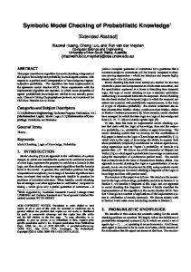
with S initialized to S init . If Top(α) = k, Bot(α) = l, and i ∈ S, then, for any j ∈ Nα (i) we have j = (iK , ..., ik+1 , jk , ..., jl , il−1 , ...i1 ). Thus, we descend from the root of the MDD encoding the current S and, only when encountering a node hk|pi we call the recursive function Fire(α, hk|pi) to compute the resulting node at the same level k using the information encoded by Wα,k ; furthermore, after processing a node hl|qi, with l = Bot(α), the recursive Fire calls stop. In [8], we gained further efficiency by performing in-place updates of (some) MDD nodes. This is based on the observation that, for any other i0 ∈ S whose last k components coincide with those of i and whose first K − k components (i0K , ..., i0k+1 ) lead to the same node hk|pi as (iK , ..., ik+1 ), we can immediately conclude that j0 = (i0K , ..., i0k+1 , jk , ..., jl , il−1 , ...i1 ) is also reachable. Thus, we performed an iteration of the form (let Ek = {α : Top(α) = k}) repeat for k = 1 to K do for each node hk|pi do for each α ∈ Ek do S ← S ∪ A(hk|pi) × Fire(α, hk|pi) until S does not change where the “A(hk|pi)×” operation comes at no cost, since it is implied by starting the firing of α “in the middle of the MDD” and directly updating node hk|pi. The memory and time savings due to in-place updates are compounded to those due to locality. Especially when studying asynchronous systems with “tall” MDDs (large K), this results in orders-of-magnitude improvements with respect to traditional symbolic approaches. However, even greater savings are achieved by saturation [9], a new iteration control strategy made possible by the use of structural model information. A node hk|pi is saturated if it is a fixed point with respect to firing any event that is independent of all levels above k: ∀l, k ≥ l ≥ 1, ∀α ∈ El , A(hk|pi)×B(hk|pi) ⊇ Nα ( A(hk|pi)×B(hk|pi) ). With saturation, the traditional global fixed-point iteration for the overall MDD disappears. Instead, we start saturating the node at level 1 (assuming |S init | = 1, the initial MDD contains one node per level), move up in the MDD saturating nodes, and end the process when we have saturated the root. To saturate a node hk|pi, we exhaustively fire each event α ∈ Ek in it, using in-place updates at level k. Each required Fire(α, hk|pi) call may create nodes at lower levels, which are recursively saturated before completing the Fire call itself (see Fig. 1). Saturation has numerous advantages over traditional methods, resulting in enormous memory and time savings. Once hk|pi is saturated, we never fire an event α ∈ Ek in it again. Only saturated nodes appear in the unique table and operation caches. Finally, most of these nodes will still be present in the final MDD (non-saturated nodes are guaranteed not to be part of it). In fact, the peak and final number of nodes differ by a mere constant in some models [9].

3

Structural-based CTL model checking

After having summarized the distinguishing features of the data structures and algorithms we employ for state-space generation, we now consider how to apply

Wa,3 =

Wb,3 =

I

Wa,2 =

I 

Wb,2 

010 Wa,1 =  0 0 1  Wb,1 100 firing chain new node or arc saturated node

a

e

0

0 0

01

01 a

012

1

1

0

0

e 012 1

2

b

01 012 1

c c

a

1 e

0

e

01 012

e

12

e

 0 0  Wd,2 = 0 0 0  Wd,1 = 0 0

00 10



01

I

We,2

I

We,1

012

1

1



0

01

c

 01  00  001 = 0 0 0 0 0 0 010 = 0 0 0 000

We,3 =

0 c

012

01

012

a

0

012

1

1 0

0

01

01

01

01

012

a

1

12

a

1 d

01 01

012

12

012 012

a

e e

012

1

e

1 01

01 012 01

a

01

0

1 e

1 0 0 0 0 0



0

1 e

Wd,3 =

b

0

012

1

I

0

0 a

01

1

012

0

0 a

0

e 01

  0 010 =  0 0 0  Wc,2 =  0 010 0 0 = I Wc,1 =  1 0 

0

0

012

Wc,3 =

I

12

012

12

012

012

012

1

1

1

Fig. 1: Encoding of N and generation of S using saturation: K = 3, E = {a, b, c, d, e}. Arrows between frames indicate the event being fired (a darker shade is used for the event label on the “active” level in the firing chain). The firing sequence is: a (3 times), b, c (at level 1), a (interrupting c, 3 times to saturate a new node), c (resumed, at level 2), e (at level 1) a (interrupting e, 3 times to saturate a new node) e (resumed, at level 2), b (interrupting e), e (resumed, at level 3), and finally d (the union of 0 1 2 and 0 1 2 at level 2, i.e., 0 1 2 , is saturated by definition). There is at most one unsaturated node per level, and the one at the lowest level is being saturated.

them to symbolic model checking. CTL [12] is widely used due to its simple yet expressive syntax and to the existence of efficient algorithms for its analysis [6]. In CTL, operators occur in pairs: the path quantifier, either A (on all paths) or E (there exists a path), is followed by the tense operator, one of X (next), F (future, or finally), G (globally, or generally), and U (until). Of the eight possible pairings, only a generator (sub)set needs to be implemented in a model checker, as the remaining operators can be expressed in terms of those in the set [13]. {EX, EU, EG} is such a set, but the following discusses also EF for clarity. 3.1 The EX operator Semantics: i0 |= EXp iff ∃i1 ∈ N (i0 ) s.t. i1 |= p. (“|=” means “satisfies”) In our notation, EX corresponds to the inverse function of N , the previousstate function, N −1 . With our Kronecker matrix encoding, the inverse of Nα is

simply obtained by transposing the matrices Wα,k in the Kronecker W incidence N T . product, thus N −1 is encoded as α∈E K≥k≥1 Wα,k To compute the set of states where EXp is satisfied, we can follow the same idea used to fire events in an MDD node during our state-space generation: given the set P of states satisfying formula p, we can accumulate the effect of “firing backward” each event by taking advantage of locality and in-place updates. This results in an efficient calculation of EX. Computing its reflexive and transitive closure, that is, the backward reachability operator EF , is a much more difficult challenge, which we consider next. 3.2 The EF operator Semantics: i0 |= EF p iff ∃n ≥ 0, ∃i1 ∈ N (i0 ), ..., ∃in ∈ N (in−1 ) s.t. in |= p. In our approach, the construction of the set of states satisfying EF p is analogous to the saturation algorithm for state-space generation, with two differences. T Besides using the transposed incidence matrices Wα,k , the execution starts with the set P, not a single state. These differences do not affect the applicability of saturation, which retains all its substantial time and memory benefits. 3.3 The EU operator Semantics: i0 |= E[p U q] iff ∃n ≥ 0, ∃i1 ∈ N (i0 ), ..., ∃in ∈ N (in−1 ) s.t. in |= q and im |= p for all m < n. (in particular, i |= q implies i |= E[p U q]) The traditional computation of the set of states satisfying E[p U q] uses a least fixed point algorithm. Starting with the set Q of states satisfying q, it iteratively adds all the states that reach them on paths where property p holds (see Algorithm EUtrad  in Fig. 2). The number of iterations to reach the fixed point
is maxi∈Sb min n | ∃ i0 ∈ Q ∧ ∀ 0 < m ≤ n, ∃ im ∈ N −1 (im−1 ) ∩ P ∧ i = in . EUtrad (in P, Q : set of state) : set of state 1. declare X , Y : set of state; 2. X ← Q; • initialize X with all states in Q 3. repeat 4. Y ← X; 5. X ← X ∪ (N −1 (X ) ∩ P); • add predecessors of states in X that are in P 6. until Y = X ; 7. return X ; Fig. 2: Traditional algorithm to compute the set of states satisfying E[p U q].

Applying saturation to EU. As the main contribution of this paper, we propose a new approach to computing EU based on saturation. The challenge in applying saturation arises from the need to “filter out” states not in P (line 5 of Algorithm EUtrad ): as soon as a new predecessor of the working set X is obtained, it must be intersected with P. Failure to do so can result in paths to Q that stray, even temporarily, out of P. However, saturation works in a highly localized manner, adding states out of breadth-first-search (BFS) order.

ClassifyEvents(in X : set of state, out EU , ES : set of event) 1. ES ← ∅; EU ← ∅; • initialize safe and unsafe sets of events 2. for each event α ∈ E • determine safe and unsafe events, the rest are dead 3. if (∅ ⊂ Nα−1 (X ) ⊆ X ) 4. ES ← ES ∪ {α}; • safe event w.r.t. X 5. else if (Nα−1 (X ) ∩ X 6= ∅) 6. EU ← EU ∪ {α}; • unsafe event w.r.t. X EUsat(in P, Q : set of state) : set of state 1. declare X , Y : set of state; 2. declare EU , ES : set of event; 3. ClassifyEvents(P ∪ Q, EU , ES ); 4. X ← Q; 5. Saturate(X , ES ); • initialize X with all states at unsafe distance 0 from Q 6. repeat 7. Y ← X; 8. X ← X ∪ (NU−1 (X ) ∩ (P ∪ Q)); • perform one unsafe backward BFS step 9. if X 6= Y then 10. Saturate(X , ES ); • perform one safe backward saturation step 11. until Y = X ; 12. return X ; Fig. 3: Saturation-based algorithm to compute the set of states satisfying E[p U q].

Performing an expensive intersection after each firing would add enormous overhead, since our firings are very lightweight operations. To cope with this problem, we propose a “partial” saturation that is applied to a subset of events for which no filtering is needed. These are the events whose firing is guaranteed to preserve the validity of the formula p. For the remaining events, BFS with filtration must be used. The resulting global fixed point iteration interleaves these two phases (see Fig. 3). The following classification of events is analogous to, but different from, the visible vs. invisible one proposed for partial order reduction [1]. b S init , E, N ), an event α is dead with Definition 1 In a discrete state model (S, respect to a set of states X if there is no state in X from which its firing leads to a state in X , i.e., Nα−1 (X ) ∩ X = ∅ (this includes the case where α is always disabled in X ); it is safe if it is not dead and its firing cannot lead from a state not in X to a state in X , i.e., ∅ ⊂ Nα−1 (X ) ⊆ X ; it is unsafe otherwise, i.e., Nα−1 (X ) \ X 6= ∅ ∧ Nα−1 (X ) ∩ X 6= ∅. 2 Given a formula E[p U q], we first classify the safety of events through static analysis. Then, each EU fixed point iteration consists of two backward steps: BFS on unsafe events followed by saturation on safe events. Since saturation is in turn a fixed point computation, the resulting algorithm computes a nested fixed point. Note that the operators used in both steps are monotonic (the working set X is increasing), a condition for applying saturation and in-place updates. Note 1 Dead events can be ignored altogether by our EUsat algorithm, since the working set X is always a subset of P ∪ Q.

Note 2 The Saturate procedure in line 10 of EUsat is analogous to the one we use for EF , except that it is restricted to a subset ES of events. Note 3 ClassifyEvents has the same time complexity as one EX step and is called only once prior to the fixed point iterations. Note 4 To simplify the description of EUsat, we call ClassifyEvents with the filter P ∪ Q, i.e., ES = {α : ∅ ⊂ Nα−1 (P ∪ Q) ⊆ P ∪ Q}. With a slightly more complex initialization in EUsat, we could use instead the smaller filter P, i.e., ES = {α : ∅ ⊂ Nα−1 (P) ⊆ P}. In practice, both sets of events could be computed. Then, if one is a strict superset of the other, it should be used, since the larger ES is, the more EUsat behaves like our efficient EF saturation; otherwise, some heuristic must be used to choose between the two. Note 5 The number of EUsat iterations is 1 plus the “unsafe distance from P to 0 Q”, maxi∈P (min{n|∃i ∈ R∗S (Q)∧∀0 < m ≤ n, ∃im S ∈ R∗S (RU (im−1 )∩P)∧i = in }), S −1 where RS (X ) = α∈ES Nα (X ) and RU (X ) = α∈EU Nα−1 (X ) are the sets of “safe predecessors” and “unsafe predecessors” of X , respectively. Lemma 1 Iteration d of EUsat finds all states i at unsafe distance d from Q. Proof. By induction on d. Base: d = 0 ⇒ i ∈ R∗S (Q) which is a subset of X (lines 4,5). Inductive step: suppose all states at unsafe distance m ≤ d are added to X in the mth iteration. By definition, a state i at unsafe distance d+1 satisfies: ∃i0 ∈ R∗S (Q) ∧ ∀0 < m ≤ d + 1, ∃jm ∈ RU (im−1 ) ∩ P, ∃im ∈ R∗S (jm ), and i = id+1 . Then, im and jm are at unsafe distance m. By the induction hypothesis, they are added to X in iteration m. In particular, id is a new state found in iteration d. This implies that the algorithm must execute another iteration, which finds j d+1 as an unsafe predecessor of id (line 8). Since i is either jd+1 or can reach it through safe events alone, it is added to X (line 10). 2 Theorem 1 Algorithm EUsat returns the set X of states satisfying E[p U q]. Proof. It is immediate to see that EUsat terminates, since its working set is a b which is finite. Let Y be the set of states monotonically increasing subset of S, satisfying E[p U q]. We have (i) Q ⊆ X (line 4) (ii) every state in X can reach a state in Q through a path in X , and (iii) X ⊆ P ∪ Q (lines 8,10). This implies X ⊆ Y. Since any state in Y is at some finite unsafe distance d from Q, by Lemma 1 we conclude that Y ⊆ X . The two set inclusions imply X = Y. 2 Figure 4 illustrates the way our exploration differs from BFS. Solid and dashed arcs represent unsafe and safe transitions, respectively. The shaded areas encircle the explored regions after each iteration of EUsat, four in this case. EUtrad would instead require seven iterations to explore the entire graph (states are aligned vertically according to their BFS depth). Note 6 Our approach exhibits “graceful degradation”. In the best case, all events are safe, and EUsat performs just one saturation step and stops. This happens for example when p∨q ≡ true, which includes the special case p ≡ true. As E[true U q] ≡ EF q, we simply perform backward reachability from Q using saturation on the entire set of events. In the worst case, all events are unsafe, and EUsat performs the same steps as EUtrad . But even then, locality and our Kronecker encoding can still substantially improve the efficiency of the algorithm.

unsafe distance: 0

distance:

0

1

1

2

2

3

3

4

5

6

Fig. 4: Comparing BFS and saturation order: distance vs. unsafe distance.

3.4 The EG operator Semantics: i0 |= EGp iff ∀n > 0 , ∃in ∈ N (in−1 ) s.t. in |= p. In graph terms, consider the reachability subgraph obtained by restricting the transition relation to states in P. Then, EGp holds in any state belonging to, or reaching, a nontrivial strongly connected component (SCC) of this subgraph. Algorithm EGtrad in Fig. 5 shows the traditional greatest fixed point iteration. It initializes the working set X with all states in P and gradually eliminates states that have no successor in X until only the SCCs of P and their incoming paths along states in P are left. The number of iterations equals the maximum length of any path over P that does not lead to such an SCC. Applying saturation to EG. EGtrad is a greatest fixed point, so to speed it up we must eliminate unwanted states faster. The criterion for a state i is a conjunction: i should be eliminated if all its successors are not in P. Since it considers a single event at a time and makes local decisions that must be globally correct, it would appear that saturation cannot be used to improve EGtrad . However, Fig. 5 shows an algorithm for EG which, like [2, 20], enumerates the SCCs by finding forward and backward reachable sets from a state. However, it uses saturation, instead of breadth-first search. In line 2, Algorithm EGsat disposes of selfloop states in P and of the states reaching them through paths in P (selfloops can be found by performing EX using a modified set of matrices Wα,k where off-diagonal entries are set to zero). Then, it chooses a single state i ∈ P and builds the backward and forward reachable sets from i restricted to P, using EUsat and ESsat (ES is the dual in the past of EU ; it differs from EUsat only in that it does not transpose the matrices Wα,k ). If X and Y have more than just i in common, i belongs to a nontrivial SCC and all of X is part of our answer C. Otherwise, we add i to the set T of trivial SCCs (i might nevertheless reach a nontrivial SCC, in Y, but we have no easy way to tell). The process ends when P has been partitioned into C, containing nontrivial SCCs and states reaching them over P, and T , containing trivial SCCs. EGsat is more efficient than our EGtrad only in special cases. An example is when the EUsat and ESsat calls in EGsat find each next state on a long path of trivial SCCs through a single lightweight firing, while EGtrad always attempts firing each event at each iteration. In the worst case, however, EGsat

EGtrad (in P : set of state) : set of state 1. declare X , Y : set of state; 2. X ← P; 3. repeat 4. Y ← X; 5. X ← N −1 (X ) ∩ P; 6. until Y = X ; 7. return X ;

EGsat(in P : set of state) : set of state 1. declare X , Y, C, T : set of state; 2. C ← EUsat(P, {i ∈ P : i ∈ N (i)}); 3. T ← ∅; 4. while ∃i ∈ P \ (C ∪ T ) do 5. X ← EUsat(P \ C, {i}); 6. Y ← ESsat(P \ C, {i}); 7. if |X ∩ Y| > 1 then 8. C ← C ∪ X; 9. else 10. T ← T ∪ {i}; 11. return C;

Fig. 5: Traditional and saturation-based EG algorithms.

can be much worse than not only EGtrad , but even an explicit approach. For this reason, the next section discusses only EGtrad , which is guaranteed to benefit from locality and the Kronecker encoding.

4

Results

We implemented our algorithms in SmArT [7] and compared them with NuSMV (version 2.1.2), on a 2.2 GHz Pentium IV Linux workstation with 1GB of RAM. Our examples are chosen from the world of distributed systems and protocols. Each system is modeled in the SmArT and NuSMV input languages. We verified that the two models are equivalent, by checking that they have the same sets of potential and reachable states and the same transition relation. We briefly describe the chosen models and their characteristics. Detailed descriptions can be found in [7]. The randomized asynchronous leader election protocol solves the problem of designating a unique leader among N participants by sending messages along a unidirectional ring. The dining philosophers and the round robin protocol models solve a specific type of mutual exclusion problem among N processes. The slotted ring models a communication protocol in a network of N nodes. The flexible manufacturing system model describes a factory with three production units where N parts of each of three different types move around on pallets (for compatibility with NuSMV, we had to change immediate events in the original SmArT model [7] into timed ones). This is the only model where the number of levels in the MDD is fixed, not depending on N (of course, the size of the local state spaces Sk , depends instead on N ). All of these models are characterized by loose connectivity between components, i.e., they are examples of globally-asynchronous locally-synchronous systems. We used the best known variable ordering for SmArT and NuSMV (they coincide in all models except round robin, where, for best performance, NuSMV uses the reverse of the one for SmArT). The time to build the encoding of N is not included in the table; while this time is negligible for our Kronecker encoding, it can be quite substantial for NuSMV, at times exceeding the reported runtimes.

State-space generation NuSMV SmArT N

|S|

time mem time mem Leader: K = 2N , |E| = N 2 + 13N 3 8.49×102 0.1 2 0.04