the motion manifold and learning a decomposable generative model. We use nonlinear ...... [15] Qiang Wang, Guangyou Xu, and Haizhou Ai. Learning object ...
Style Adaptive Bayesian Tracking Using Explicit Manifold Learning Chan-Su Lee and Ahmed Elgammal Computer Science Department Rutgers, The State University of New Jersey Piscataway, NJ 08854, USA Email:{chansu, elgammal}@cs.rutgers.edu Abstract
Characteristics of the 2D contour shape deformation in human motion contain rich information and can be useful for human identification, gender classification, 3D pose reconstruction and so on. In this paper we introduce a new approach for contour tracking for human motion using an explicit modeling of the motion manifold and learning a decomposable generative model. We use nonlinear dimensionality reduction to embed the motion manifold in a low dimensional configuration space utilizing the constraints imposed by the human motion. Given such embedding, we learn an explicit representation of the manifold, which reduces the problem to a one-dimensional tracking problem and also facilitates linear dynamics on the manifold. We also utilize a generative model through learning a nonlinear mapping between the embedding space and the visual input space, which facilitates capturing global deformation characteristics. The contour tracking problem is formulated as states estimation in the decomposed generative model parameter within a Bayesian tracking framework. The result is a robust, adaptive gait tracking with shape style estimation.
1 Introduction Vision-based human motion tracking and analysis systems have promising potentials for many applications such as visual surveillance in public area, activity recognition, and sport analysis. Human motion involves not only geometric transformations but also deformations in shape and appearance. Characteristics of the shape deformation in a person motion contain rich information such as body configuration, person identity, gender information, and even emotional states of the person. Human identification [4] and gender classification [5] are examples of the applications. There have been a lot of work on contour tracking such as active shape models (ASM) [3], active contours [10], and exemplar-based tracking [14]. It is still hard to get robust contour tracking and in the same time be able to adapt to different people being tracked with automatic initialization. Modeling dynamics of shape and appearance is essential for tracking human motion. The observed human shape and appearance in video sequences goes through complicated global nonlinear deformation between frames. If we consider the global shape, there are two factors affecting the shape of the body contour through the motion: global dynamics factor and
person shape style factor, The dynamic factor is constrained because of dynamics of the motion and the physical characteristics of human body configuration [12, 1]. The person shape style is time-invariant factor characterizing distinguishable features in each person shape depending on body built(big, small, short, tall, etc.). These two factors can summarize rich characteristics of human motion and identity. Our objective is to achieve trackers that can track global deformation in contours and can adapt to different people shapes automatically . There are several challenges to achieve this goal. First, modeling the human body shape space is hard, considering both the dynamics and the shape style. Such shapes lie on a nonlinear manifold. Also, in some cases there are topological changes in contour shapes through motion which makes establishing correspondences between contour points unfeasible. Second, how to simplify the dynamics of the global deformation. Can we learn a dynamic model for body configuration that is low in dimensionality and exhibits linear dynamics? For certain classes of motion like gait, facial expression and gestures, the deformation might lie on a low dimensional manifold if we consider a single person. Our previous work [7] introduced a framework to separate the motion from the style in a generative fashion where the motion is represented in a low dimensional representation. In this paper we utilize a similar generative model within a Bayesian tracking formulation that is able to track contours in cluttered environment where the tracking is performed in three conceptually independent spaces: body configuration space, shape style space and geometric transformation space. Therefore, object state combines heterogeneous representations. The challenge will be how to represent and handle multiple spaces without falling into exponential increase of the state space dimensionality. Also, how to do tracking in a shape space which can be high dimensional? We present a new approach for tracking nonlinear global deformation in human motion based on Bayesian tracking with emphasis on the the gait motion. Our contributions are as follows: First, by applying explicit nonlinear manifold learning and its parametric representation, we can find compact, low dimensional representation of body configuration which reduces the complexity of the dynamics of the motion into a linear system for tracking gait. Second, by utilizing conceptually independent decomposed state representation, we can achieve approximation of state posterior estimation in a marginalized way. Third, the adaptive tracking of person shape allows not only tracking of any new person contour but also shows potential for identification of the person during tracking. As a result, we achieve robust, adaptive gait tracking with style estimation from cluttered environment. The paper organization is as follows. Section 2 summarizes the framework. Section 3 describes the state representation and learning. Section 4 describes the the tracking framework. Section 5 shows some experimental results.
2 Framework We can think of the shape of a dynamic object as instances driven from a generative model. Let zt ∈ Rd be the shape of the object at time instance t represented as a point in a ddimensional space. This instance of the shape is driven from a model in the form zt = Tαt γ (bt ; st ),
(1)
where the γ (·) is a nonlinear mapping function that maps from a representation of the body configuration bt into the observation space given a mapping parameter st that characterizes the person shape in a way independent from the configuration and specific for the person
st
st−1 bt
bt−1
yt
yt−1 αt−1
αt zt
zt−1
Figure 1: Graphic model for decomposed generative model
being tracked. Tαt represents a geometric transformation on the shape instance. Given this generative model, we can fully describe observation instance zt by state parameters αt ,bt , and st . Figure 1 shows a graphical model illustrating the relation between these variables where yt is a contour instance generated from model given body configuration bt and shape style st and transformed in the image space through Tαt to form the observed contour. The mapping γ (bt ; st ) is a nonlinear mapping from the body configuration state bt as yt = A × st × ψ (bt ),
(2)
where ψ (bt ) is a kernel induced space, A is a third order tensor, sk is a shape style vector and × is appropriate tensor product as defined in [11]. The tracking problem is then an inference problem where at time t we need to infer the body configuration representation bt and the person specific parameter st and the geometric transformation Tαt given the observation zt . The Bayesian tracking framework enables a recursive update of the posterior P(Xt |Z t ) over the object state Xt given all observation Z t = Z1 , Z2 , .., Zt up to time t: Z t
P(Xt |Z ) ∝ P(Zt |Xt )
Xt−1
P(Xt |Xt−1 )P(Xt−1 |Z t−1 )
(3)
In our generative model, the state Xt is [αt , bt , st ], which uniquely describes the state of the tracking object. Observation Zt is the captured image instance at time t. The state Xt is decomposed into three sub-states αt , bt , st . These three random variables are conceptually independent since we can combine any body configuration with any person shape style with any geometrical transformation to synthesize a new contour. However, they are dependent given the observation Zt . It is hard to estimate joint posterior distribution P(αt , bt , st |Zt ) for its high dimensionality. The objective of the density estimation is to estimate states αt , bt , st for a given observation. The decomposable feature of our generative model enables us to estimate each state by a marginal density distribution P(αt |Z t ), P(bt |Z t ), and P(st |Z t ). We approximate marginal density estimation of one state variable along representative values of the other state variables. For example, in order to estimate marginal density of P(bt |Z t ), we estimate P(bt |αt∗ , st∗ , Z t ), where αt∗ , st∗ are representative values such as maximum posteriori estimates.
(b) a unified manifold (c) generated sequences
(a) individual manifolds 2 2
1.5
1.5
1.5
2
1
1.5
0.5
1
0
0.5
1
1
0.5
0.5
0
0
−0.5
−0.5
−0.5
0
−1
−0.5
−1 −2
−1
−1.5
2
−1.5 −2 2 1.5
0
−2 −2
1 0
−1 1 0.5
0 −0.5 −1 −1.5 2 −2
0 1
−1 2 −2
−1.5 2
−1 1
−1.5 −2
0 −1 −2 −2
−1
0
1
2
−1 0 1 2
2
1
0
−1
−2
Figure 2: Individual manifolds and their unified manifold
3 Learning Generative Model Our objective is to establish generative models for the shape in the form of equation 2 where the intrinsic body configuration is decoupled from the shape style. Such model was introduced in [7] and applied to gait data and facial expression data. Given training sequences of different people performing the same motion (gait in our case), Locally Linear Embedding (LLE) [13] is applied to find low dimensional representation of body configuration for each person manifold. As a result of nonlinear dimensionality reduction, an embedding of the gait manifold can be obtained in a low dimensional Euclidean space where three is the least dimensional space where the two halves of the walking cycles can be discriminated. Figure 2-a shows low dimensional representation of side-view walking sequences for different people. Generally, the walking cycle evolves along a closed curve in the embedded space, i.e., only one degree of freedom controls the walking cycle which corresponds to the constrained body pose as a function of the time. Such manifold can be used as intrinsic representation of the body configuration. The use of LLE to obtain intrinsic configuration for tracking was previously reported in [15]. Modeling body configuration space: Body configuration manifold is parameterized using a spline fitted to the embedded manifold representation. First, cycles are detected given an origin point on the manifold by computing geodesics along the manifold. Second, a meanmanifold for each person is obtained by averaging difference cycles. Obviously, each person will have a different manifold based on his spatio-temporal characteristics. Third, non-rigid transformation using an approach similar to [2] is performed to find a unified manifold representation as in Fig. 2-b . Correspondences between different subjects are accomplished by selecting a certain body pose as the origin point in different manifolds and equal sampling in the parameterized representation. Finally, we parameterized the unified mean manifold by spline fitting. The unified mean-manifold can be parameterized by a one-dimensional parameter βt ∈ R and a spline fitting function f : R → R3 that satisfies bt = f (βt ) is used to map from the parameter space into the three dimensional embedding space. Fig. 2-c shows three sequences generated using the same equidistant body configuration parameter [β1 , β2 , · · · , β16 ] along the unified mean manifold with different style. As a result of one dimensional representation of each cycle in unified manifold, aligned body pose can be generated in different shape style. Modeling style shape space: Shape style space is parameterized by a linear combination of basis of the style space. First, RBF nonlinear mappings [7] are learned between the embedded body configuration bt on the unified manifold and corresponding shape observations ytk for each person k. The mapping has the form ytk = γk (bt ) = Ck · ψ (bt ), where Ck is the mapping coefficients which depend on particular person shape and ψ (·) is a nonlinear mapping with N
RBF kernel functions to model the manifold in the embedding space. Given learned nonlinear mapping coefficients C1 ,C2 , · · · ,CK , for training people 1, · · · , K, the shape style parameters are decomposed by fitting an asymmetric bilinear to the coefficient space. As a result, we can generate contour instance ytk for particular person k at any body configuration bt as ytk = A × sk × ψ (bt ),
(4)
where A is a third order tensor, sk is a shape style vector for person k. Ultimately the style parameter s should be independent of the configuration and therefore should be time invariant and can be estimated at initialization. However, we don’t know the person style initially and , therefore, the style needs to fit to the correct person style gradually during the tracking. So, we formulated style as time variant factor that should stabilize after some frames from initialization. The dimension of the style vector depends on the number of people used for training and can be high dimensional. We represent new style as a linear combination of style classes learned from the training data. The tracking of the high dimensional style vector st itself will be hard as it can fit local minima easily. A new style vector s is represented by linear weighting of each of the style classes sk , k = 1, · · · , K using linear weight λ k : K
s=
∑ λ k sk ,
k=1
K
∑ λ k = 1,
(5)
k=1
where K is the number of style classes used to represent new styles. Modeling geometric transformation space: Geometric transformation in human motion has constraints. We parameterize the geometric transformation by scaling Sx , Sy and translation Tx , Ty . New representation of any contour point can be found using homogeneous transformation α with paramters [Tx , Ty , Sx, Sy] as global transformation parameters. The overall generative model can be expressed as # ! Ã " K
zt = Tαt
A×
∑ λtk sk
× ψ ( f (βt )) .
(6)
k=1
Tracking problem using this generative model is the estimation of parameter αt , βt , and λt at each new frame given the observation zt .
4
Bayesian Tracking
4.1 Marginalized Density Representation Since it is hard to estimate joint distribution of high dimensional data, we represent each of the sub-state densities by marginalized ones. We approximate the marginal density of each sub-state using maximum a posteriori (MAP) of the other sub-states, i.e., P(αt |Zt ) ∝ P(αt |bt ∗ , st ∗ , Zt ), P(bt |Zt ) ∝ P(bt |αt ∗ , st ∗ , Zt ), P(st |Zt ) ∝ P(st |αt ∗ , bt ∗ , Zt ), (7) where αt ∗ , bt ∗ , and st ∗ are maximum a posteriori estimate of each approximated marginal density. Maximum a posteriori of the joint density Xt∗ = [αt∗ , bt∗ , st∗ ] = arg maxXt P(Xt |Z t ) will maximize the posterior marginal densities αt∗ = arg maxαt P(αt |Z t ), bt∗ = arg maxbt P(bt |Z t ), and st∗ = arg maxst P(st |Z t ) because of our decomposable generative model.
Dynamic Models
P(αt |αt−1 ) = N(H αt−1 , σα
2)
P(bt |bt−1 ) ∝ P(βt |βt−1 ) = N(βt + v, ˜ σb 2 ) P(st |st−1 ) ∝ P(λt |λt−1 ) = N(st−1 , σs t2 )
Predicted States (i) αˆ t ∝ P(αt |αt−1 ) ( j) βˆt ∝ P(βt |βt−1 ) (k) λˆ t ∝ P(λt |λt−1 ) ∝ P(st |st−1 )
Table 1: Dynamic models and predicted density of states
4.2 Dynamic Model The dynamic model P(Xt |Xt−1 ) = P(αt , bt , st |αt−1 , bt−1 , st−1 ) predicts the state Xt at time t given the previous state Xt−1 . In our generative model, the states are decomposed into three different factors. In the Bayesian network shown in Fig. 1, the transitions of each of the substates are independent. Therefore, we can describe whole state dynamic model by dynamic models of individual sub-states as P(αt , bt , st |αt−1 , bt−1 , st−1 ) = P(αt |αt−1 )P(bt |bt−1 )P(st |st−1 ).
(8)
In case of body configuration, the manifold spline parameter βt will change in a constant speed if the subject walks in a constant speed (because it corresponds to constant frame rate used in the learning). However, the resulting manifold point representing body configuration bt = f (βt ) will move along the manifold in different step sizes. Therefore, we use βt to model the dynamics since it results in a one dimensional linear dynamic system. In general, the walking speed can change gradually. So, the body configuration in each new state will move from the current state with a filtered speed that is adaptively estimated during the tracking. Dynamic model of style is approximated by a random walk as the style may change smoothly around specific person style. The global transformation αt captures global contour motion in the image space. The left column in table 1 shows the dynamic models, where v˜ is filtered estimated body configuration manifold velocity, and H is a transition matrix of the geometric transformation state which is learned from the training data. A new sub-state densities can be predicted using each sub-state dynamic models as in table 1 right column .
4.3
Tracking Algorithm using Particle Filter
We represent state densities using particle filters since such densities can be non-Gaussian and the observation is nonlinear. In particle filter, the density of posterior P(Xt |Z t ) is approx(i) (i) (i) (i) imated by a set of N weighted samples {Xt , πt }, where πt is the weight for particle Xt . Using the generative model in Eq. 6, the tracking problem is to estimate αt , λt , and βt for given observation Z t . The marginalized posterior densities for αt , βt , and λt are approximated by particles. (i) (i) α ( j) ( j) Nb (k) (k) s {αt , α πt }Ni=1 , {βt , b πt } j=1 , {λt , s πt }Nk=1 , (9) where Nα ,Nb , and Ns are the numbers of particles used for each of the sub-states. Density representation P(β |Z t ) is interchangeable with P(bt |Z t ) as it has one to one correspondence ( j) ( j) between βt and bt . The same holds between λt and st for the style state. We estimate states by sequential update of the marginalized sub-densities utilizing the predicted densities of the other sub-states. These densities are updated with current observation Zt by updating weighting values of each sub-state particles approximation using the
observation. We estimate global transformation αt using predicted density s`t , b` t . Then body configuration bt is estimated using estimate global transformation αt , and predicted density s`t . Finally style st is estimated with given estimated αt , and bt . The following table summarizes the state estimation procedure using time t − 1 estimation. 1. Importance-sampling with resampling: (i) (i) Nα ( j) ( j) (k) (k) b s , {βt−1 , b πt−1 }Nj=1 t − 1 state density estimation: {αt−1 , α πt−1 }i=1 , {λt−1 , s πt−1 }N k=1 . (i) ( j) (k) Resampling: {α` t−1 , 1/Nα }, {β`t−1 , 1/Nb }, and {λ` t−1 , 1/Ns }. 2. Predictive update of state densities: (i) (i) αt = H α` t−1 + N(0, σα2 ) ( j) ( j) ( j) ( j) β = β` + v˜t + N(0, σb 2 ), b = f (β ) t (k)
λt
t (k)
t−1
(k) 2 ), = λ` t−1 + N(0, σs t−1
λt
t
(k)
λt
=
N
(k)
,
(k)
s λ ∑i=1 i
st
t
(k)
s = ∑N i=1 λi
t si
3. Sequential update of state weights using current observation: Global transformation αt with bˆ t , sˆt : (i) (i) (i) P(αt |bˆ t∗ , sˆt∗ , Zt ) ∝ P(Zt |αt , bˆ t∗ , sˆt∗ )P(αt ) α (i) (i) (i) (i) πt α π = P(Z |α , b ˆ t∗ , sˆt∗ ), α πt = t t ( j) t N
α απ ∑ j=1 t
Body pose bt with αt , sˆt : (i∗ ) (i) αt∗ = αt , where i∗ = arg maxi α πt ( j)
( j)
( j)
( j)
P(bt |αt∗ , sˆt∗ , Zt ) ∝ P(Zt |αt∗ , bt , sˆt∗ )P(bt ) b πt Style st with αt , bt : ( j∗ ) ( j) bt∗ = bt , where j∗ = arg max j b πt (k)
(k)
( j)
= P(Zt |αt∗ , bt , sˆt∗ ),
b π ( j) t
=
b ( j) πt
N
(i)
b bπ ∑i=1 t
(k)
P(st |αt∗ , bt∗ , Zt ) ∝ P(Zt |αt∗ , bt∗ , st )P(st ) s π (k) t
(k) = P(Zt |αt∗ , bt∗ , st ),
s π (k) t
=
s (k) πt Ns s (i) πt ∑i=1
4.4 Observation Model (i)
( j)
(k)
In our multi-state representation, we update weights α πt , b πt , and s πt by marginal(i) ( j) (k) ized likelihood P(Zt |αt , bt , st∗ ), P(Zt |αt∗ , bt , st∗ ), and P(Zt |αt∗ , bt∗ , st ) given observation Zt . Each sub state captures different characteristics in the dynamic motion and affects different variations in the observation. For example, body poses are changed according to body configuration state. Different body configurations show significant changes in edge direction in the legs. However, in case of style, the variation is subtle and changes along the global contours. (i) Observation model measures state Xt by updating the weights πt in the particle filter by (i) measuring the observation likelihood P(Zt |Xt ). We can estimate the likelihood by µ ¶ µ ¶ d(Zt , zt ) d(Zt , Tαt A × st × ψ (bt )) P(Zt |Xt ) = P(Zt |αt , bt , st ) ∝ exp − = exp − , (10) σt2 σt2 where d(·) is distance measure, zt is the contour from the generative model using αt , bt , st . It is very important to use proper distance measurement d(·) in order to get accurate update of weights and density for new observation. We use three distance measures: Chamfer distance, weighted Chamfer distance, and oriented Chamfer distance. Representation: We represent shape contour by an implicit function similar to [6] where the contour is the zero level of such function. From each new frame Zt , we extracted edge using Canny edge detector algorithm.
Weighted Chamfer Distance for Geometric Transformation Estimation: For geometric transformation estimation, the predicted body configuration, and style estimate from the previous frame are used. Therefore, we need to find similarity measurement which is robust to the deviation of body pose and style estimation and sensitive to global transformation. Typically the shape or the silhouette of upper body part in walking sequence are relatively invariant to the body pose and style. By giving different weight to different contour points in Chamfer matching, we can emphasize upper body part and de-emphasize lower body part in the distance measurement. Weighted chamfer distance can be computed as Dw (T, F,W ) =
1 N min ρ (ti , fi )wi , N∑ i fi ∈F
(11)
where ti is i’th feature location, fi template feature and wi i’th feature weight. Practically, weighted chamfer distance achieved more robust estimation of the geometric transformation. Oriented Chamfer Distance for Body Pose: Different body poses can be characterized by the orientation of legs. Therefore, oriented edge based similarity measurement is useful in case of the body configuration estimation. Oriented chamfer distance matching was used in [8]. We use a linear filter [9] to detect oriented edge efficiently after edge detection. After applying the linear filter to the contour and the observation, we applied chamfer matching for each oriented distance transform and oriented contour template. The final result is the sum of each of the oriented chamfer distance. For style estimation, simple Chamfer distance is used.
5
Experimental Result
We used CMU Mobo data set for learning the generative model, the dynamics, and for testing the tracker. Six subjects are used in learning the model. The tracking performance is evaluated for people used in training and for unknown people, which were not used in the learning. We initialize the tracker by giving a rough estimate of initial global transformation parameter. The body configuration is initialized by random particles along the manifold. In case of style, as we don’t know the subject style from the initial frame, we initialize style by mean style, which means equal weights are applied for every style class. Tracking for trained subjects : For the training subjects, the tracker shows very good tracking results. It shows accurate tracking of body configuration parameter βt and correct estimation of shape style st . Fig. 3 (a) shows several frames during tracking known subject. The left column shows tracking contours. The middle column shows the posterior body configuration density. The right column is the estimated style weights in each frame. Fig. 3 (b) shows tracking results for style weights. The figure shows that the style estimate converges to the subject’s correct style and it becomes the major weighting factor after about 10 frames. The style weighting shows accurate identification of the subject as a result of tracking and it has many potential for human identification and others. Fig. 3 (c) shows estimated body configuration β value. Even though the two strides making each gait cycle are very similar and hard to differentiate in visual space, the body configuration parameter accurately find out the correct configuration. The figure shows that the body configuration correctly exhibits linear dynamics. As we have one to one mapping between body configuration on the manifold and 3D body pose, we can directly recover 3D body configuration using the estimated β or using manifold points bt similar to [6]. Tracking for unknown subjects: Tracking for new subjects can be hard as we used small number of people for learning style in the generative model. It takes more frames to converge
(a) tracking of subject 2
16th frame:
4th frame:
64th frame:
1
1
1
1
1
1
0.9
0.9
0.9
0.9
0.9
0.9
0.8
0.8
0.8
0.8
0.8
0.8
0.7
0.7
0.4
0.4
0.4
0.4
0.3
0.3
0.3
0.3
0.3
0.3
0.2
0.2
0.2
0.2
0.2
0.2
0.1
0.1
0.1
0.1
0.1
0.1
0 0
0.5 1 Body Configuration: βt
0.5
0.5
0.4
0.4
0
0.6
0.6
0.5
0.5
0.7
0.7
0.6
0.6
0.5
0.5
0.7
0.7
0.6
0.6
0 1
2 3 4 5 Shape style
0
6
0
0.5 1 Body Configuration: βt
(b) style weights
0 1
2 3 4 5 Shape style
0
6
0
0.5 1 Body Configuration: βt
1
2 3 4 5 Shape style
6
(c) body configuration βt 1
0.9 0.9
0.8 0.8
0.7 style style style sytle sytle style
0.5 0.4
0.7
1 2 3 4 5 6
Body configuration βt
Style weights
0.6
0.3
0.5 0.4 0.3
0.2 0.1
0.2
0 −0.1 0
0.6
0.1
20
40
60
80 100 120 Frame number
140
160
180
0 0
200
20
40
60
80 100 120 Frame number
140
160
180
200
Figure 3: Tracking for known person (a) tracking of unknown subject
16th frame:
4th frame:
64th frame:
1
1
1
1
1
1
0.9
0.9
0.9
0.9
0.9
0.9
0.8
0.8
0.8
0.8
0.8
0.8
0.7
0.7
0.7
0.7
0.7
0.7
0.6
0.6
0.5
0.5
0.6
0.6
0.5
0.5
0.4
0.4
0.4
0.4
0.3
0.3
0.3
0.3
0.3
0.3
0.2
0.2
0.2
0.2
0.2
0.2
0.1
0.1
0.1
0.1
0.1
0.1
0 0
0.5 1 Body Configuration: β
0 1
t
0.5
0.5
0.4
0.4
0
0.6
0.6
2 3 4 5 Shape style
0
6
0
0.5 1 Body Configuration: β t
(b) style weights
0 1
2 3 4 5 Shape style
0
6
0
0.5 1 Body Configuration: β
1
t
2 3 4 5 Shape style
6
(c) body configuration βt style style style sytle sytle style
0.9 0.8
1 2 3 4 5 6
1 0.9 0.8
0.7 0.7
Body configuration βt
Style weights
0.6 0.5 0.4 0.3
0.1
0.5 0.4
0.2
0 −0.1 0
0.6
0.3
0.2
0.1
20
40
60
80 100 120 Frame number
140
160
180
200
0 0
20
40
60
80 100 120 Frame number
140
160
180
200
Figure 4: Tracking for unknown person to accurate contour fitting as shown in Fig. 4 (b). However, after some frames it accurately fit to the subject contour even though we did not do any local deformation to fit the model to the subject. There is no one dominant style class weight during the tracking and sometimes the highest weight are switched depend on the observation. In case of the body configuration βt , you can see sometimes it jumps about half cycle due to the similarity in the observation since the style is not accurate enough. Still, the result shows accurate estimation of body pose. We also, applied tracking in normal walking situation using M. Black straight walking person image sequence even though we learned the generative model from treadmill walking data. Fig. 5 shows contour tracking results for 40 frames. Fig. 5 (c) shows estimated body configuration parameters. It confused in some intervals at the beginning but it recovers within the cycle.
6 Conclusion We presented new framework for human motion tracking using a decomposable generative model. As a result of our tracking, we not only find accurate contour from cluttered envi-
10th frame:
40th frame:
style weights:
body configuration βt : 1
style 1 style 2 style 3 sytle 4 sytle 5 style 6
0.9 0.8
0.9 0.8
0.7 0.7
0.6 0.6
0.5 0.5
0.4
0.4
0.3
0.3
0.2
0.2
0.1
0.1
0 −0.1 0
5
10
15
20
25
30
35
40
0 0
5
10
15
20
25
30
35
40
Figure 5: Tracking straight walking ronment without background learning or appearance model, but also get parameters for body configuration and shape style. In current work, we assumed fixed view in learning the generative model and tracking human motion. We plan to extend the model to view variant situations. We used marginalized density approximation instead of full joint distribution of the state. Sampling based on Markov Chain Monte Carlo (MCMC) can be used for more accurate estimation of the marginal density. In our current system, we tried to overcome the problem in marginalization by finding robust distance measure in the observation and sequential estimation using predicted density.
References [1] Richard Bowden. Learning statistical models of human motion. In Proc. IEEE Workshop on Human Modeling, Analysis and Synthesis, pages 10–17, 2000. [2] H. Chui and A. Rangarajan. A new algorithm for non-rigid point matching. In Proc. IEEE CVPR, pages 44–51, 2000. [3] T.F. Cootes, D. Cooper, C.J. Taylor, and J. Graham. Active shape models - their training and application. Computer Vision and Image Understanding, 61(1):38–59, 1995. [4] David Cunado, Mark S. Nixon, and John Carter. Automatic extraction and description of human gait models for recognition purposes. Computer Vision and Image Understanding, 90:1–41, 2003. [5] James W. Davis and Hui Gao. An expressive three-mode principal components model for gender recognition. Journal of Vision, 4(5):362–377, 2004. [6] Ahmed Elgammal and Chan-Su Lee. Inferring 3d body pose from silhouettes using activity manifold learning. In Proc. IEEE CVPR, pages 681–688, 2004. [7] Ahmed Elgammal and Chan-Su Lee. Separating style and content on a nonlinear manifold. In Proc. IEEE CVPR, pages 478–485, 2004. [8] D.M. Gavrila. Multi-feature hierarchical template matching using distance transforms. In Proc. IEEE ICPR, pages 439–444, 1998. [9] Rafael C. Gonzalez and Richard E. Woods. Digital Image Processing. Addison Wesley, 1992. [10] Michael Isard and Andrew Blake. Condensation–conditional density propagation for visual tracking. Int.J.Computer Vision, 29(1):5–28, 1998. [11] Lieven De Lathauwer, Bart de Moor, and Joos Vandewalle. A multilinear singular value decomposition. SIAM Journal On Matrix Analysis and Applications, 21(4):1253–1278, 2000. [12] D. Ormoneit, H. Sidenbladh, M. J. Black, T. Hastie, and D. J. Fleet. Learning and tracking human motion using functional analysis. In Proc. IEEE Workshop on Human Modeling, Analysis and Synthesis, pages 2–9, 2000. [13] Sam Roweis and Lawrence Saul. Nonlinear dimensionality reduction by locally linear embedding. Science, 290(5500):2323–2326, 2000. [14] Kentaro Toyama and Andrew Blake. Probabilistic tracking in a metric space. In Proc. IEEE ICCV, pages 50–57, 2001. [15] Qiang Wang, Guangyou Xu, and Haizhou Ai. Learning object intrinsic structure for robust visual tracking. In Proc. of CVPR, pages 227–233, 2003.