multiple-access decoding problem, for which we apply superposition coding. ..... of random codes with a rate that is greater than 1 â h(W), we ensure that the ...
Superposition Coding for Side-Information Channels∗ Amir Bennatan†
David Burshtein†
Tel-Aviv University, Israel
Tel-Aviv University, Israel
Giuseppe Caire‡ Formerly with Eurecom Institute, France. Currently with the University of Southern California
Shlomo Shamai‡ Technion, Israel
Abstract We present simple, practical codes designed for the binary and Gaussian dirty-paper channels. We show that the dirty paper decoding problem can be transformed into an equivalent multiple-access decoding problem, for which we apply superposition coding. Our concept is a generalization of the nested lattices approach of Zamir, Shamai and Erez. In a theoretical setting, our constructions are capable of achieving capacity using random component codes and maximum-likelihood decoding. We also present practical implementations of the constructions, and simulation results for both dirty-paper channels. Our results for the Gaussian dirty-paper channel are on par with the best known results for nested-lattices. We discuss the binary dirty-tape channel, for which we present a simple, effective coding technique. Finally, we propose a framework for extending our approach to general Gel’fand-Pinsker channels.
Index Terms - dirty paper, dirty tape, multiple-access channel, side information, superposition coding. ∗ †
IEEE Transactions on Information Theory, volume 52, no. 5, pp. 1872-1889, May 2006. The first two authors were supported by the Israel Science Foundation, grant no. 22/01-1, by an equipment
grant from the Israel Science Foundation to the school of Computer Science in Tel Aviv University and by a fellowship from The Yitzhak and Chaya Weinstein Research Institute for Signal Processing at Tel Aviv University. ‡ The last two authors were supported by the EU 6th framework programme, via the NEWCOM network of excellence.
1
I
Introduction
Side-information channels were first considered by Shannon [43]. Such channels are characterized by an input X, output Y and state-dependent transition probability p(y|x, s) where the channel state S is i.i.d., known to the transmitter and unknown to the receiver. Shannon [43] considered the case of state sequence known causally. Kusnetsov and Tsybakov [32] were the first to consider the case of state sequence known non-causally, and Gel’fand and Pinsker [29] obtained the capacity formula for this case. The binary and Gaussian side-information channels are given by Y =X +S+Z
(1)
With binary side-information channels, addition is over the binary field F2 . The random variable S is referred to as interference (following [21]) and constitutes the channel state, which is known to the encoder. In this paper we assume S to be i.i.d. with uniform probability P (S = 0) = P (S = 1) = 1/2. Z is binary symmetric noise, distributed as Bernoulli(p), and X is the channel input, subject to an input constraint 1/n · dH (x, 0) ≤ W , where dH (x, y) denotes Hamming distance between two n-vectors x and y. With Gaussian side-information channels, addition in (1) is over the real number field. The channel input X is subject to a power constraint PX , i.e. 1/n · kxk2 ≤ PX , where kxk2 denotes the square-distance norm of x. The noise Z is distributed as a zero-mean Gaussian variable with variance PZ . S is the known interference. We make no assumptions on the distribution of S. Following Costa’s “Writing on Dirty Paper” famous title [17], when the interference S is known non-causally, these channels are referred to as “dirty paper” channels. By analogy, the case of causally known interference is called “dirty tape” (see e.g. [9]). Costa was the first to examine the Gaussian dirty paper problem. He obtained the remarkable result that the interference, known only to the encoder, incurs no loss of capacity in comparison with the standard interference-free channel. Costa assumed that S is Gaussian i.i.d distributed. This result was extended in [16] and [21] to arbitrarily distributed interference. Pradhan et al. [39] and Barron et al. [3] obtained the capacity of the binary dirty paper channel. Unlike the Gaussian dirty paper channel, here a penalty is paid for the interference known only to the transmitter. Applications for side-information problems include data-hiding (see [14, 19, 36, 25]), where a host signal is modelled as interference, and a watermark is modelled as an additive transmitted signal X subject to a maximum distortion constraint. In the binary case, the host signal is typically a black and white image, or the least-significant bit-layer of a gray-scale image, and the 2
signal is received through some memoryless transformation modelled as a BSC. In the Gaussian case the signals are allowed to be continuous, and the memoryless transformation is modelled as AWGN. Other applications of dirty tape include precoding for channels with ISI [21], where ISI is modelled as interference known causally at the encoder. Transmission over broadcast channels is an important application of dirty paper coding [11]. This application is particularly pronounced in the case of the MIMO Gaussian broadcast channel, see [52]. The achievability of capacity in dirty paper channels is proven by means of a random construction of codes and a random partition of their codewords into “bins”. This method typically produces unstructured codes, which are infeasible for practical implementation. Zamir, Shamai and Erez [54] suggested a framework for introducing structure into the above “random binning” method. Their technique involves nested codes (and nested lattices). That is, they use a fine code C and a coarse code C0 such that C0 ⊂ C. Their construction requires that the fine code C be designed as a good channel-code, while the coarse code C0 must be designed to be a good source-code. LDPC codes are likely candidates for codes C and C0 . However, although LDPC codes are well suited for channel coding, the problem of finding a good source-coding algorithm for them remains open. Unless such an algorithm is found, the codes in their current form are unsuitable for selection as C0 . We would like to select C as an LDPC code, but the nested structure of C and C0 means that the codes are entangled in a way that restricts the independent selection of C. One approach for challenging this problem was considered by Philosof et al. [38, 37] and Erez and ten Brink [23] using coset dilution. In this paper we present an alternative to the nested lattices method of [54] using superposition of codes, which enables independent selection of a quantization and an information-bearing code. We begin in Section II by presenting superposition-coding for the binary dirty-paper channel. We define the codes used and discuss encoding and decoding. We also show that in a randomcoding setting, using minimum-distance encoding and maximum-likelihood decoding, our codes are capable of achieving capacity. Such constructions are not realizable in practice, but provide motivation and insight for the design of practical codes, as discussed later. Of particular importance is the insight provided by the analogy between our scheme’s decoding problem and the problem of decoding over a multiple-access channel (MAC). In Section III, we extend our scheme to the Gaussian dirty-paper channel. Our development follows closely in the lines of the binary dirty-paper case. In Section IV we briefly discuss codes for dirty-tape channels. These codes serve as an important benchmark for the performance of
3
more complex codes for dirty-paper channels. In Section V we show how the constructions of Sections II and III can be transformed to produce powerful codes for practical implementation. We discuss the selection of the component codes of our scheme, and the design of encoders and decoders. We also provide simulation results that confirm the effectiveness of our scheme. In Section VI we propose a framework for the extension of superposition-coding to the general Gel’fand-Pinsker (noncausal side-information) problem. Our discussion is designed primarily to generate interest, while further research is required to produce practical results. Section VII concludes the paper.
II
Superposition Coding for Binary Dirty Paper
II.1
Definition
Like the nested-lattices approach of [54], our approach begins with two codes: C0 and C1 , referred to as the quantization code and the information-bearing code, respectively. The superposition code C is defined as C = C0 + C1 , i.e., C = {c = c0 + c1 : c0 ∈ C0 , c1 ∈ C1 }
(2)
In a random-coding setting (as will be discussed in Section II.2), we construct the quantization code C0 by random i.i.d selection according to a Bernoulli(1/2) distribution. The informationbearing code C1 is constructed by random i.i.d selection according to a Bernoulli(q) distribution, where q is a parameter that will be discussed later. The codes are constructed at rates R0 and R1 , respectively, and block length n. In the practical application of the scheme (Section V.1), the codes will be selected differently, relying on insight provided by the random-coding discussion. Encoding and decoding for the binary dirty-paper channel proceed as follows. Encoder: The encoder selects a codeword c1 ∈ C1 , and sends the sequence x = [c1 + s]C0 where s is the interference vector, and [y]C = y + QC (y). For any y ∈ Fn2 , QC (y) is defined by ∆
∆
QC (y) = arg minc∈C dH (y, c). ∆
Defining c0 = QC0 (c1 + s), we may also write, x = c1 + s + QC0 (c1 + s) = c0 + c1 + s
4
The channel outputs the signal y = x + s + z = c0 + c1 + z
(3)
ˆ1 ) such that c ˆ0 +ˆ ˆ1 is announced Decoder: The decoder computes the pair (ˆ c0 , c c1 is closest to y. c as the decoded codeword. Note that the encoder begins by selecting a codeword c1 ∈ C1 , and decoding terminates by ˆ1 . Thus the effective rate of the transmission scheme is the rate R1 of C1 . producing c The operation of the decoder is identical to that of a decoder for the additive multiple-access (MAC) channel where two virtual users with codebooks C0 and C1 send independently selected codewords c0 and c1 , respectively. This choice of decoder is motivated by the observation that since s is uniformly distributed over Fn2 and is independent of c1 , the codeword c0 is independent of c1 . The analogy with the MAC channel has an important function in the design of practical decoders, that will be discussed in Section V. It is instructive to consider the above superposition scheme in terms of the random-binning achievability scheme of Gel’fand and Pinsker [29]. In [29], a random codebook C is constructed, and its codewords are randomly partitioned into bins (subsets) {Cm : m = 1, . . . , M }, where M is the number of distinct messages that may be transmitted. Each message is associated with a bin, and encoding begins by selecting a bin Cm to match with the transmitted message m. The encoder proceeds to search within Cm for a codeword c that is “nearest” (in terms of joint-typicality) to the interference vector s. The transmitted vector x is a function of s and c. ˆ that is “nearest” (again, in terms The decoder searches the entire code C for the codeword c ˆ and of joint-typicality) to the received y. It then determines the unique bin Cˆm that contains c declares the decoded message m ˆ to be the one matching the bin. With superposition coding, the codebook C is given by the superposition code C0 + C1 . For each codeword c1 ∈ C1 , the coset code c1 + C0 = {c1 + c0 : c0 ∈ C0 } is equivalent to a bin of [29]. Encoding begins by selecting a codeword c1 ∈ C1 . This selection is equivalent to the selection of the bin c1 + C0 . The operation of evaluating QC0 (c1 + s) can equivalently be presented as a search, over the coset code c1 + C0 , for the word c = c1 + c0 that is nearest to s. The transmitted vector is x = c − s (subtraction being evaluated over F2 , and is identical to addition). Assuming the code C0 is dense “enough” (a precise analysis of which will be provided in Section II.2 below), the nearest codeword c will be close to s, and the transmitted difference x between the two vectors will not violate the Hamming input constraint. The channel adds s to x, and thus the result is equivalent to the transmission of c = c0 + c1 . 5
The channel also adds the unknown noise z, so the resulting output is y = c + z = c0 + c1 + z. ˆ=c ˆ0 + c ˆ1 that is nearest to y. The decoder searches the superposition code C for the codeword c ˆ=c ˆ0 + c ˆ1 , Assuming that C is not “too” dense, the correct codeword c will be recovered. Given c ˆ1 identifies the bin c ˆ1 + C0 to which c ˆ belongs. c It is interesting to note on the case of nonuniform interference S, i.e. S here is distributed as Bernoulli(s) where s 6= 1/2. This is an instance of the general noncausal side-information channel whose capacity was evaluated by Gel’fand and Pinsker [29] and is given by C = sup {I(U ; Y ) − I(U ; S)}
(4)
p(u|s)
where U is an auxiliary random variable with conditional distribution p(u|s) and X is a deterministic function of S and U , X = f (S, U ). In our case of nonuniform binary dirty paper, the capacity achieving p(u|s) and f (s, u) are unknown. However, consider the case U = S + X, where X is distributed as Bernoulli(W ). This choice of U is interesting because it produces an achievable rate I(U ; Y )−I(U ; S) that is greater than the capacity in the uniform interference case (the expression for which will be given in Section II.2). But with this choice, U is not uniformly distributed in {0, 1}. Thus, the capacity-achieving scheme prescribes bins that are different to the ones constructed in this section. This problem of generating codewords according to nonuniform distributions was considered in various contexts (see e.g. [7] which discusses the Slepian-Wolf problem, [51] which discusses binning in a theoretical context and [35] in the context of wideband Gel’fand-Pinsker channels). An approach that is based on superposition coding is proposed in Section VI.
II.2
Random Coding Analysis
We now provide a precise analysis of superposition coding using randomly generated codes. In this section we assume an encoder-decoder pair that uses minimum-distance quantization and maximum-likelihood decoding. As noted in Section I, when unstructured codes (like the above discussed random codes) are applied, such an encoder-decoder pair is not realizable in practice. The same applies to our development in Section III.2, where we will discuss superposition coding for the Gaussian dirty-paper channel in a random-coding setting. In Section V we will discuss the implementation of our approach in a practical setting. Our analysis in this section parallels that of Erez, Shamai and Zamir [21, 54] with nested lattices. They proved that the nested-lattices approach can be used to enable reliable transmission at rates arbitrarily close to the dirty-paper capacity. However, their analysis, like ours, assumed 6
optimal lattices and an encoder-decoder pair that are not realizable in practice, at rates approaching channel capacity. The main purpose of their discussion was to motivate the interest in the nested-lattices approach. Similarly, an important objective of the developments in this section and in Section III.2, is to show that there is no loss of optimality that is necessarily incurred by parting with the highly structured lattice constructions of [54]. The developments thus provides motivation for the development of Section V, where codes that are unsuitable for constructing lattices are successfully applied to the dirty-paper problem1 . An important additional objective is to provide important insight that will guide the practical design of codes in Section V. We construct C0 and C1 as discussed in Section II.1. We define an encoder error as the event that the transmitted x violates the codeword constraint, i.e. dH (x, 0) > nW . A decoder error b1 6= c1 . The error probability of the scheme is the probability of the union of these two occurs if c
events. We begin with an analysis of the probability of an encoder error: Lemma 1 The probability of an encoder error approaches zero with n, if R0 satisfies R0 > 1 − h(W )
(5)
where h(·) denotes the binary entropy function2 . The proof of this lemma relies on the following observation: Since s is uniformly distributed over
Fn2 and independent of c1 , then also c1 + s is uniformly distributed over Fn2 . R(W ) = 1 − h(W ) is the binary Hamming-weight rate-distortion function [18]. Hence, by choosing C0 in the ensemble of random codes with a rate that is greater than 1 − h(W ), we ensure that the encoder will find a codeword at distance at most nW from c1 + s with an ensemble average probability that approaches 1 as n → ∞. Now consider the probability of a decoder error. Given the formal analogy with the MAC (Section II.1), we can conclude that the probability of a decoder error vanishes with n if the rate pair (R0 , R1 ) lies within the capacity region of the MAC. This condition is sufficient, i.e., it yields an achievability result. In fact, the decoder is only interested in reliable decoding of C1 , while in the MAC both C1 and C0 must be reliably decoded. However, as we shall see in the following, for an appropriate choice of the parameter q governing the ensemble of C1 , the additional condition 1 2
This point is further explained in Section III.3. Note that throughout this paper, we measure rate in bits, and hence the base of the log function is always 2,
including in the expression for h(·).
7
of decoding reliably also C0 incurs no loss of optimality. We therefore proceed to the following lemma, Lemma 2 Consider the MAC Y = X0 + X1 + Z
(6)
where all variables are over F2 , where Z is binary noise distributed as Bernoulli(p), and where user 1 is subject to a Hamming weight input constraint q. The capacity region is given by all pairs (R0 , R1 ) ∈ R2+ satisfying R1 ≤ h(p ⊗ q) − h(p) R1 + R0 ≤ 1 − h(p)
(7)
∆
where p ⊗ q = p(1 − q) + q(1 − p). The proof of this lemma is provided in Appendix A. Finally, we combine Lemmas 1 and 2 to obtain: Theorem 1 If R0 and R1 satisfy (5) and (7) then the average probability of error approaches zero with the block length n. Note that the code C0 has dual requirements to be both a good quantization code (to enable effective encoding) and a good channel code (for effective decoding). Since the averaged probabilities of encoder and decoder errors both approach zero with n, we are ensured that most codes in the random-coding ensemble are good in both senses. Fig. 1 presents the capacity region prescribed by Theorem 1. A dashed line marks the constraint imposed by (5). Transmission is possible at any point that is within the MAC capacity region and is above the dashed line. This is the achievable region of superposition coding. The MAC capacity region is a function of parameters q and p. To show that superposition coding can achieve capacity, we must show that we can select q such that this region contains a point (R0 , R1 ) where R1 (the effective rate) equals the capacity C of the dirty-paper channel, (1). The expression for C (see Pradhan et al. [39] and Barron et al. [3]) is given by, C=
h(W ) − h(p)
for Wc ≤ W ≤ 1/2
αW
for 0 ≤ W ≤ Wc
(8)
where Wc = 1 − 2−h(p) and α = log((1 − Wc )/Wc ). Note that in the range 0 ≤ W ≤ Wc , capacity is achieved by time-sharing, with a duty-cycle θ = W/Wc , of the standard random-binning scheme 8
for Hamming distortion equal to Wc and “silence” (zero rate and zero Hamming distortion)3 . We select q such that q ⊗ p ≥ W . For any W ≤ 1/2 there exists q ? ∈ [0, 1/2] such that this condition holds for all q ≥ q ? . With this selection of q, we obtain that the rate pair R0 = 1 − h(W ), R1 = h(W ) − h(p) falls within the MAC capacity region. Thus, pairs of quantization and information-bearing codes C0 and C1 can be found such that the resulting scheme achieves rates arbitrarily close to h(W ) − h(p), as desired (capacity in the range 0 < W < Wc is again obtained by time-sharing).
R0 1 − h(p)
Achievable Region
R1 = h(W ) − h(p)
1 − h(W )
h(p ⊗ q) − h(p)
R1
Figure 1: Capacity region of the corresponding binary MAC channel.
III III.1
Superposition Coding for Gaussian Dirty Paper Definition
We now extend superposition coding to the Gaussian dirty paper problem. We again consider two codes, a quantization code C0 and an information-bearing code C1 . The superposition code is defined as C = C0 + C1 mod A (addition being the standard addition over the real-number field), ∆
where the operation mod A is applied componentwise as follows: Given a scalar x, x mod A = x − QA (x) such that QA (x) is the nearest multiple of A to x. The dynamic range of x is thus reduced to [−A/2, A/2]. 3
Unlike the case of Gaussian channel studied by Costa [17] and examined in Section III, the binary dirty paper
capacity is strictly less than the capacity if interference was not present, which is given by C = h(p ⊗ W ) − h(p).
9
The modulo-A operation is borrowed from the construction-A approach to generating lattices from linear codes. Its effect can be equivalently modelled as the tessellation of the entire space
Rn with replicas of the n-dimensional cube [−A/2, A/2]n . Note that it must not be confused with the modulo-lattice operation of nested lattices scheme of [54], which serves a different purpose. In a random-coding setting (as will be discussed in Section III.2), we construct the quantization code C0 by random i.i.d selection according to a uniform distribution in the range [−A/2, A/2]. The information-bearing code C1 is constructed by random i.i.d selection according to a zeromean distribution with a variance Q (Q is a parameter that will be determined later). The exact distribution will be discussed in Appendix B and approaches a Gaussian distribution as A → ∞. C0 and C1 have rates R0 and R1 , respectively, and block length n. Encoder: The encoder selects a codeword c1 ∈ C1 , and sends the sequence: x = [αs + d − c1 mod A]C0 mod A A and α are arbitrary constants that will be discussed later. d is a randomly selected dither signal, borrowed from the nested lattices approach of [54]. However, unlike [54], the elements of the dither are defined to be uniformly i.i.d in the range [−A/2, A/2]. This dither corresponds to the dither of Philosof et al. [38]. ∆
[ξ]C0 = QC0 (ξ) − ξ, QC0 (ξ) being the codeword of C0 that is closest to ξ assuming a modulo A distance metric. The mod A distance between two vectors x and y is given by ky − xk2A = ∆
n X
(yi − xi mod A)2
i=1
We thus obtain, x = [QC0 (αs + d − c1 mod A) − (αs + d − c1 )] mod A = c0 + c1 − αs − d mod A ∆
where c0 = QC0 (αs + d − c1 mod A). Our choice of C0 will be shown in Section III.2 to be capable of quantization with a mean square distortion PX , assuming mod A distance. Thus x is guaranteed to satisfy the power constraint, 1/n ·
Pn
2 i=1 xi
≤ PX .
The received signal is y =x+s+z Decoder: The decoder computes 10
ˆ y
=
∆
αy + d mod A
=
c0 + c1 − (1 − α)x + αz mod A
=
ˆ mod A c0 + c1 + z
(9)
ˆ is z ˆ = −(1 − α)x + αz. The decoder evaluates the pair (ˆ ˆ1 ) such where the effective noise z c0 , c ˆ0 + c ˆ1 is closest to y ˆ , assuming mod A distance. c ˆ1 is announced as the decoded codeword. that c ¿From the above construction, it is clear that c0 and c1 are independent, implying the analogy ˆ contains a “self-noise” element x that, for to the MAC channel. However, the effective noise z particular choices of the codes C0 and C1 , is not independent of c0 and c1 , undermining an assumption of the Gaussian MAC model. In Section III.2 we show that under a random-coding assumption, the MAC model is valid and a decoder designed for the MAC channel is capable of achieving capacity. In section V we show that the analogy is valuable in a practical setting as well.
III.2
Random Coding Analysis
As in our analysis of superposition coding for binary dirty-paper, we now analyze the scheme for the Gaussian channel using randomly generated codes. The purpose of this section is once again to provide motivation and guidelines to a construction using practical codes, which is discussed in Section V. We assume that C0 and C1 are constructed as in Section III.1. In Theorem 2 (below) we consider the probability of error. The proof, which is provided in Appendix B, employs an encoder/decoder pair that rely on joint-typicality instead of the minimum-distance metrics that were used in Section III.1. However, it is important to note that the decoder is similar to the MAC decoder that is used in information-theoretic proofs [18] (the only difference being that it ∆
ˆ = αy and decodes tests for strong-typicality instead of weak-typicality). The decoder evaluates y ˆ0 and c ˆ1 assuming a virtual MAC channel c Yˆ = U0 + U1 + Zˆ mod A
(10)
where U0 and U1 are virtual, independent users and Zˆ is independent zero-mean Gaussian noise with variance PZˆ = (1 − α)2 PX + α2 PZ . Thus, the theorem reinforces the analogy to the MAC channel. In the sequel, we further assume that the MAC channel is characterized by a power constraint Q on user 1, paralleling our development in Section II.2.
11
Theorem 2 Given the above selection of C0 and C1 , an encoder/decoder pair can be designed such that the following holds: 1. The probability of an encoder error (i.e., a violation of the power constraint) approaches zero with the block length n, if R0 satisfies R0 > log A −
1 log(2πePX ) + δ1 2
(11)
where δ1 → 0 as A → ∞. 2. The probability of a decoder error approaches zero with n if the pair (R0 , R1 ) lies in the interior of the capacity region of the MAC channel, whose transition probabilities are determined by (10), and where user 1 is subject to the power constraint Q. This capacity region is given by, 1 log(2πePZˆ ) + δ2 ! Ã 2 1 Q + δ3 log 1 + 2 PZˆ
(12)
R0 + R1 ≤ log A − R1 ≤
(13)
where δ2 , δ3 → 0 as A → ∞.
R0
log A − 21 log(2πePZˆ )
log A − 12 log(2πePX )
Achievable Region
X R1 = 21 log( P PZˆ )
1 log(1 + Q ) 2 PZˆ
R1
Figure 2: Capacity region of the corresponding AWGN MAC channel.
The proof of the theorem is provided in Appendix B. Fig. 2 is similar to Fig. 1 and presents the capacity region prescribed by Theorem 2. A dashed line marks the constraint imposed by equation (11) (neglecting elements δ1 ,δ2 and δ3 ). Transmission is possible at any point that is within the MAC capacity region and is above the dashed line. 12
In a manner similar to the binary dirty paper case, the MAC capacity region is a function not only of the power constraint PX and the noise variance PZ but also of parameters α and Q. As in Section II.2, our desire is to select α and Q such that a point (R0 , R1 ) where R1 = 1/2 log(1 + PX /PZ ) falls within the achievable region. Combining equations (11) and (12), we obtain, R1
I(U ; S)
(18)
2. The probability of a decoder error approaches zero with n if the pair (R0 , R1 ) lies in the interior of the following achievable region for the MAC channel whose transition probabilities are determined by (17). R0 + R1 ≤ I(U ; Y ) R1 ≤ I(U ; Y ) − I(V0 ; Y )
(19) (20)
where I(V0 ; Y ) is a term that depends on p(v1 ), whose precise definition is provided in Appendix F.1. An outline of the proof of the theorem is provided in Appendix F.1. Note that the bounds in the theorem are similar to the bounds in Theorems 1 and 2. The MAC achievable region is a function of the term I(V0 ; Y ). This term is affected by the choice of p(v1 ), which determined the random generation of C1 . It is our objective to design p(v1 ) 24
such that the point R1 = I(U ; Y ) − I(U ; S) (the achievable rate of the Gel’fand-Pinsker channel for a given choice of U ) and R0 = I(U ; S) lies within this achievable region. To avoid being bounded away from capacity by (20), we must select p(v1 ) such that I(V0 ; Y ) ≤ I(U ; S). Several such choices for p(v1 ) are discussed in Appendix F.2. So far, our discussion assumed randomly constructed codes. In a practical setting, we would typically select the code C0 as a convolutional code or trellis code, and C1 to be an LDPC code. Using the Viterbi algorithm, the encoder would seek the codeword c0 that maximizes Pr[s | δ(c1 + c0 )] =
Qn
i=1 Pr[S
= si | U = δ(c1,i + c0,i )], where we have applied the above defined relation
p(s | u). The decoder, using joint BCJR and LDPC belief-propagation decoding, would seek a pair of codewords c0 and c1 such that Pr[y | δ(c0 + c1 )] =
VII
Qn
i=1 Pr[yi
| δ(c1,i + c0,i )] is maximized.
Conclusion
Superposition coding provides a simple approach to constructing codes for the binary and Gaussian dirty-paper problems. This simplicity produces several advantages. For example, the component codes are not required to be building-blocks of a lattice, and hence are allowed to be nonlinear, adding an extra degree of freedom to their design. The simple structure of superposition-codes also lends itself to the simple design of codes and decoders, as demonstrated in Section V. An important element of our analysis has been the analogy between our scheme’s decoding problem and the decoding problem over a MAC channel. This analogy has enabled the utilization, in Section V, of a wide body of research that exists for the design of practical decoders for the MAC channel. In Section V we have presented promising simulation results for the binary and Gaussian dirty paper channels. In particular, the results for the Gaussian dirty-paper channel indicate reliable transmission within 1.2 dB of the Shannon limit, at a rate of 0.25 bits per real dimension, and within 1 dB of the Shannon limit at a rate of 0.5 bits per real dimension. These results are the same as the best reported results with nested lattices [23]. Superposition coding was recently applied by Sun et al. [45] (using a stronger trellis code and a different design approach for the decoder) to obtain codes capable of reliable transmission within 0.88 dB of the Shannon limit at 0.25 bits per real dimension. The approach presented in this paper assumes scalar interference channels. However, the approach may easily be applied to a vector MIMO setting by decomposing the vector channel into an array of scalar channels, exactly as performed by Telatar [46][Section 3.1] in the context
25
of the no-interference channel13 . A different method for extending our approach to the vector MIMO setting was recently suggested by Lin et al. [34]. Superposition-coding relies on a close relation between the dirty-paper channel and the multipleaccess channel. Interestingly, a relationship between these two problems has recently been observed by Vishwanath et al. [50] who obtained a duality between the MIMO broadcast dirty-paper achievable region and the MIMO MAC capacity region.
Appendix A
Proof of Lemma 2
For any input product distribution p(x0 , x1 ) = p(x0 )p(x1 ), define the region R(p(x0 )p(x1 )) given by R0 ≤ I(X0 ; Y |X1 ) R1 ≤ I(X1 ; Y |X0 ) R0 + R1 ≤ I(X0 , X1 ; Y )
(21)
The capacity region of the MAC (6) is given by the closure of the convex hull of the union of all regions R(p(x0 )p(x1 )), for all p(x0 )p(x1 ) satisfying the input constraint, i.e., for which p(x1 ) satisfies
E[dH (X1 , 0)] ≤ q We observe that I(X1 ; Y |X0 ) ≤ h(p ⊗ q) − h(p)
(22)
since the RHS in (22) is the capacity of the input-constrained BSC Y = X1 +Z (under conditioning with respect to X0 , the contribution of user 0 can be removed from the received signal). We observe also that I(X0 ; Y |X1 ) ≤ 1 − h(p)
(23)
since the RHS in (23) is the capacity of the BSC Y = X0 + Z. Finally, we observe that I(X0 , X1 ; Y ) = H(Y ) − h(p) ≤ 1 − h(p) 13
(24)
The decomposition, as well as the allocation of power to the individual scalar channels, is performed as though
no interference was present. After the decomposition, dirty-paper coding proceeds using a modified interference, resulting from a multiplication of the vector of interference components by a fixed unitary matrix.
26
By letting p(x1 ) be Bernoulli(q) and p(x0 ) be Bernoulli(1/2), the upper bounds (22), (23) and (24) are simultaneously achieved. Since the resulting region is closed and convex, no closure and convex hull operations are needed.
B
2
Proof of Theorem 2
In this proof, we consider the following channel model: Y = X + S + Z mod A/α
(25)
Y in this model corresponds to the channel output as in (9) after the modulo operation was performed, but without multiplication by α. Hence the argument to the modulo operation is A/α instead of A. For simplicity of our model, we encapsulate the random known dither into the interference S, and assume that the interference is uniformly distributed in the range [−A/(2α), A/(2α)]. We begin by defining the following set of random variables. X is Gaussian with variance PX . The distribution of U1 will be defined later in this section. The variables S, X and U1 are independent. We also define U0 to satisfy the equation: U0 = αS + X − U1 mod A
(26)
Hence, U0 is uniformly distributed in the range [−A/2, A/2] and is dependent on S, X and U1 . Note that X is identical to a similar definition by Costa [17]. U0 and U1 replace Costa’s auxiliary U . The code C0 , as defined in Section III.1, corresponds to random i.i.d selection according to the distribution of U0 . The exact distribution for the random i.i.d generation of C1 in Section III.1 was left unspecified. We now define it to equal the distribution of U1 , which in turn will be specified later in this section. To simplify our analysis, we consider an encoder/decoder pair that employs joint-typicality rather than a minimum-distance metric. We begin with the encoder. Encoder: The encoder selects a codeword c1 ∈ C1 , and seeks a word c0 ∈ C0 such that the pair c0 and (αs − c1 mod A) are jointly strongly ²-typical with respect to the distribution of the random variables U0 and (αS − U1 mod A) (² will be determined later). If no such c0 is found, the encoder declares an error. Otherwise, it transmits the sequence x = c0 + c1 − αs mod A. Note that the encoder requires strong typicality. The justification for this is similar to the one in the theoretical analysis of Gel’fand and Pinsker [29] and will be clarified later. 27
To bound the probability of an encoder error, we apply Lemma 13.6.2 of [18]. The probability of an encoder error approaches zero with n if R0 satisfies R0 > I(U0 ; αS − U1 mod A) + ²1
(27)
where ²1 is some value, dependent on ² that approaches 0 with ². I(U0 ; αS − U1 mod A) = h(U0 ) − h(U0 | αS − U1 mod A) = log A − h(X mod A) The distribution of Xmod A approaches the distribution of X as A approaches infinity. Hence, I(U0 ; αS − U1 mod A) = log A −
1 log(2πePX ) + δ1 2
where δ1 → 0 as A → ∞. Thus, if (11) is satisfied, then for large enough A and small enough ², (27) is satisfied. This completes the proof of Part 1 of the theorem. We now define Yˆ = αY and combine (25) and (26) to obtain, Yˆ
= U0 + U1 − (1 − α)X + αZ mod A = U0 + U1 + Zˆ mod A
(28)
∆ ∆ where Zˆ = − (1 − α)X + αZ. Zˆ is distributed as a Gaussian variable with variance PZˆ = (1 −
α)2 PX + α2 PZ . X and Z are independent of U0 and U1 , and hence Zˆ is also independent of U0 and U1 , thus overcoming the obstacle in (9). Since C0 and C1 were constructed according to U0 and U1 , we would expect the probability of error to approach zero if (R0 , R1 ) lie within the capacity region of the MAC channel as defined in Lemma 14.3.1 of [18]. The proof, however, is slightly more involved than the proof of [18]. This is because the ˆ was not generated according to the true MAC channel model (28). Specifically, channel output y ˆ was not generated by random selection according to X. We begin by the self-noise element x of z replacing the decoder of [18] with a decoder that requires strong (rather than weak) typicality. ˆ0 ∈ C0 and c ˆ1 ∈ C1 such that the triplet (ˆ ˆ1 , y) are jointly Decoder: The decoder seeks c c0 , c strongly ²-typical with respect to the distribution of (U0 , U1 , Y ). We now consider the probability of a decoder error. 1. We start by examining the probability that the channel output y is not strongly ²-typical with the transmitted c0 and c1 . To determine the probability of this event, we examine some intermediate values. 28
We first examine the probability that the triplet (c0 , c1 , αs − c1 ) are not jointly strongly ²-typical. The random variable U1 is independent of (αS − U1 mod A) and U0 by the fact that αS is uniformly distributed in the range [−A/2, A/2]. Similarly, c1 is independent of (αs − c1 mod A). The codebook C0 was generated independently of c1 , and the selected codeword c0 is a function of (αs − c1 mod A). Hence the codeword c1 is also independent of the pair c0 and (αs − c1 mod A). Thus, by the weak law of large numbers, we obtain that the probability that c0 , c1 and (αs − c1 mod A) are jointly strongly ²-typical approaches one with n. If the triplet (c0 , c1 , αs − c1 mod A) are jointly strongly ²-typical, then so are the sequences (x, s, c0 , c1 ), because x and s are obtained from the original triplet by applying deterministic operations. Finally, in a manner similar to the analysis of Gel’fand and Pinsker [29], we observe that (U0 , U1 ), (X, S) and Y form a Markov chain and hence by the Markov lemma (see e.g. [18][Lemma 14.8.1]), y is jointly strongly ²-typical with c0 and c1 with probability that approaches 1 with n. 2. We now examine the event that there exist codewords c00 ∈ C0 and c01 ∈ C1 , other than the transmitted c0 and c1 , that are jointly strongly ²-typical with the channel output y. Lemma 4, which is provided in Appendix C extends the achievability proof of the MAC ˆ has been shown above to capacity region from [18] to our setting using the fact that y be strongly typical (with probability approaching 1) to the MAC model (28)14 . All that remains is therefore to evaluate the MAC capacity region. We replace Y of Lemma 4 by Yˆ of our discussion, as defined in (28). I(U0 ; Yˆ | U1 ) = h(Yˆ | U1 ) − h(Yˆ | U0 , U1 ) = h(U0 + Zˆ mod A) − h(Zˆ mod A) The first element of the sum is maximized by U0 that is uniformly distributed in the range [−A/2, A/2], matching our choice above. Hence h(U0 + Zˆ mod A) = log A. As A approaches ˆ Hence infinity, Zˆ mod A approaches the distribution of Z. 1 I(U0 ; Yˆ | U1 ) = log A − log 2πePZˆ + δ2 2
(29)
where δ2 → 0 as A → ∞. We proceed to examine, I(U1 ; Yˆ | U0 ) = h(U1 + Zˆ mod A) − h(Zˆ mod A) 14
ˆ is obtained from y using a deterministic invertible operation, strong typicality with y is Note that since y
ˆ. equivalent to strong typicality with y
29
For large A, the distribution for U1 that maximizes the first element of the above sum, under the restriction that the variance does not exceed Q, approaches a Gaussian random variable N (0, Q). We now define the distribution of U1 to match this maximizing distribution. Thus, I(U1 ; Yˆ | U0 ) = =
1 1 log 2πe(Q + PZˆ ) − log 2πePZˆ + δ3 2 2 Ã ! 1 Q log 1 + + δ3 2 PZˆ
(30)
where δ3 → 0 as A → ∞. Using similar arguments, ˆ I(U0 , U1 ; Yˆ ) = h(U0 + U1 + Zˆ mod A) − h(Zmod A) 1 = log A − log 2πePZˆ + δ2 2
(31)
Finally, combining (29), (30), and (31), recalling Lemma 4, we obtain the capacity region of (11) and (12), thus completing the proof of the theorem. 2
C
Statement and Proof of Lemma 4
The following lemma extends achievability proof of the MAC capacity region from [18]. It differs from the achievability proof of Theorem 14.3.1 of [18] in that it only assumes that the channel output y is typical to the MAC, and does not require that the output be truly generated by the MAC. Also, it assumes that the MAC decoder tests for strong-typicality, as in Appendices B and F.1 rather than weak-typicality as in [18]. Lemma 4 Let p(y | u0 , u1 ) be the transition probabilities of a MAC. Let U0 and U1 be two random codes generated by i.i.d selection according to distributions p(u0 ) and p(u1 ), at rates R0 and R1 (respectively). Let u0 and u1 be the transmitted codewords and y the corresponding channel output. Assume a MAC decoder that tests for joint strong ²-typicality. If (u0 , u1 , y) are jointly strongly ²-typical, then for small enough ², the ensemble probability of decoding error approaches zero with the block length n if the following inequalities hold: R0 < I(U0 ; Y | U1 ) R1 < I(U1 ; Y | U0 ) R0 + R1 < I(U0 , U1 ; Y )
30
(32)
Proof. An error occurs if there exists any other pair of codewords (u00 , u01 ) 6= (u0 , u1 ) such that (u00 , u01 , y) are jointly strongly ²-typical. We first examine the probability of a codeword u00 6= u0 being jointly strongly ²-typical with (u1 , y). Let U0 denote a random sequence, generated by i.i.d selection according to p(u0 ), independently of u1 and y. Invoking Lemma 13.6.2 of [18] we obtain, P r[(U0 , u1 , y) ∈ A∗² ] < 2−n[I(U0 ;U1 ,Y )−²1 ] where A∗² denotes the set of strongly ²-typical sequences and ²1 approaches zero as ² → 0 and n → ∞. Examining I(U0 ; U1 , Y ) we have, I(U0 ; U1 , Y ) = h(U1 , Y ) − h(U1 , Y | U0 ) = h(Y | U1 ) + h(U1 ) − [h(Y | U0 , U1 ) + h(U1 | U0 )] = h(Y | U1 ) − h(Y | U1 , U0 )] = I(U0 ; Y | U1 ) The third equality follows from the fact that U0 and U1 are independent, and hence h(U1 | U0 ) = h(U1 ). Using a union bound, we obtain, Pr[∃u00 ∈ U0 : u00 6= u0 , (u00 , u1 , y) ∈ A∗² ] < 2nR0 · 2−n[I(U0 ;Y
| U1 )−²1 ]
= 2n[R0 −I(U0 ;Y
| U1 )+²1 ]
For small enough ², the probability of this error event approaches zero with n if the first inequality in (32) is satisfied. Similarly, the probability of a codeword u01 6= u1 being jointly strongly ²-typical with (u0 , y) approaches zero if the second inequality in (32) is satisfied. Finally we have, P r[(U0 , U1 , y) ∈ A∗² ] < 2−n[I(U0 ,U1 ;Y )−²1 ] and hence the probability of two codewords u00 6= u1 and u01 6= u1 being jointly strongly ²-typical with y approaches zero if the last inequality in (32) is satisfied.
2
The application of Lemma 4 in our context of side-information channels requires a discussion of the following fine point. An underlying assumption of the lemma is that the codewords of C0 and C1 , except for the transmitted c0 and c1 , have been generated by a random selection process independently of y. This assumption is true in the context of the regular MAC channel. The reasoning is that the production of the transmitted codewords c0 and c1 and subsequently the generation of y, has no relation to the random events that produced the other codewords (2)
(M0 )
c0 , ..., c0
(2)
(M1 )
and c1 , ..., c1
of both codes.
In our case, we assume that the encoder examines the codewords of C0 by some order, and stops at the ith codeword if it is strongly typical with c1 and s. Hence, given that the encoder 31
(i)
(1)
(i−1)
selected c0 , it cannot be argued that the production of codewords c0 , ..., c0
is independent
of s and c1 . Each of the codewords is known to be not typical with s and c1 . Consequently, they are not in general independent of y. The solution to this problem is simple: Our random-coding analysis holds for codewords (i+1)
c0
(M0 )
, ..., c0
(1)
(i−1)
, since they were produced independently of y. Codewords c0 , ..., c0
are ran-
domly selected among words that are not typical with c1 and s. For large enough n, the probability that they are jointly typical with y is bounded by a multiplicative constant factor times the probability assuming independent selection. Examining the proof of Lemma 4, it is easy to verify this is sufficient for our needs. To see this, let U0 be a randomly selected sequence distributed i.i.d as p(u0 ). We first examine the probability that U0 would be jointly typical with the transmitted c1 and y, given that it was not typical with s and c1 . Pr[(U0 , c1 , y) ∈ A∗² | (U0 , c1 , s) ∈ / A∗² ] = ≤
Pr[(U0 , c1 , y) ∈ A∗² , (U0 , c1 , s) ∈ / A∗² ] Pr[(U0 , c1 , s) ∈ / A∗² ] Pr[(U0 , c1 , y) ∈ A∗² ] (1 − 2−n(I(U0 ;U1 ,S)−²1 ) )
For large enough n, the denominator is greater than 1/2. Hence we obtain, Pr[(U0 , c1 , y) ∈ A∗² | (U0 , c1 , s) ∈ / A∗² ] ≤ 2 · Pr[(U0 , c1 , y) ∈ A∗² ] Let U1 be randomly i.i.d distributed as p(u1 ), we can analyze the probability that U0 would be jointly typical with some other codeword U1 of C1 and y, given that it was not typical with s and the transmitted c1 . This case is handled in exactly the same manner as the previous one we have just examined, and is therefore omitted. The last error event of the MAC channel involves the probability that a codeword c01 , other than the transmitted c1 , would be jointly typical with c0 and y. Unlike the case of C0 , the independence of c1 from the other codewords of its codebook does carry over from the MAC model. Hence, this case does not require any special attention.
D
Joint Iterative Decoding for Superposition Codes
The joint iterative decoder used in this paper is based on the concepts of Boutros and Caire [8]. We use the terminology of factor graphs, which was introduced by Kschischang et al. [31]. Fig. 3 is a schematic diagram of the factor graph which forms the basis of the decoding process. The gray-filled circles represent channel observation nodes. The black squares are MAC factor 32
Channel observation nodes 1
1
2
2
3
3
.. .
.. .
.. . n
n
check nodes code bits
MAC factor nodes
variable nodes
Factor graph of C0
Factor graph of C1
Figure 3: Factor graph for joint iterative decoding for binary dirty-paper.
33
nodes that process the channel observations and the information obtained from one code and communicate them to the other code. The left hand side of the graph contains the factor graph of C0 . For simplicity, we have only drawn nodes corresponding to bits of the convolutional code (with binary dirty-paper) or symbols of the trellis code (with Gaussian dirty-paper). The right hand side of the graph contains the factor (Tanner) graph of C1 .
D.1
Binary Dirty-Paper
We first consider the binary dirty-paper problem. For this problem, C1 is designed to be a GQCLDPC code. As mentioned in Section V.1, GQC-LDPC codes are obtained from LDPC codes defined over Galois fields15 Fq where q ≥ 2. The non-binary symbols of the code are mapped to a binary channel alphabet using a mapping function, δ : Fq → {0, 1}. The C1 portion of the factorgraph is involved in recovering the nonbinary codeword of the Fq -LDPC code (from which the GQC-LDPC code was constructed). Thus, the nodes of this portion of the factor graph exchange vector messages among themselves and with the MAC factor nodes. C0 , on the other hand, is a binary convolutional codes. Its nodes therefore exchange scalar messages. The MAC factor nodes perform the translation between the two types of message. For example, given a vector message v = [v0 , ..., vq−1 ] from an LDPC variable node (with some abuse of notation, we let the indices 0, ..., q − 1 represent the elements of Fq ), the following scalar message s is transferred to the convolutional code: Pq−1
s = Pq−1 i=0
i=0
Pr[y | δ(i) + 1] · vi
Pr[y | δ(i) + 1] · vi +
Pq−1 i=0
Pr[y | δ(i)] · vi
(33)
where y denotes the channel output observed by the MAC factor node, δ(i) + 1 is computed over
F2 (the channel alphabet), and Pr[y | δ(i) + 1] is evaluated using the virtual MAC model, (6). When decoding begins, the variable nodes of the LDPC factor-graph transmit messages v = [1/q, ..., 1/q] to the MAC factor node, indicating zero knowledge. The factor nodes apply (33) to obtain scalar messages that are transferred to the factor graph of C0 . It is important to observe that by applying (33), the MAC factor nodes implicitly benefit from the knowledge of the mapping δ(·) and through it, of the expected weight of GQC-LDPC codewords. The convolutional code uses the scalar messages from the MAC factor nodes to perform a BCJR iteration. The BCJR algorithm is applied using the approach developed by Berrou and 15
In the definition of [4], GQC-LDPC codes are obtained from coset-Fq -LDPC codes rather than Fq -LDPC codes.
For simplicity of our discussion, we neglect the addition of a coset vector to the LDPC code. This addition can easily be accounted for by modifying expressions (33),(34), (35) and (36).
34
Glavieux [6]
16 .
With this approach, the message produced at each of the convolutional bit
nodes, and directed to a MAC factor node, does not rely on the information that was previously obtained from that factor node. Note that unlike the algorithm of [6], no distinction is made between systematic and non-systematic bits, and outgoing messages are computed for all. The MAC factor nodes translate each scalar message s into a vector message v using the following expression: vi = α · (Pr[y | δ(i) + 1] · s + Pr[y | δ(i)] · (1 − s))
(34)
where α is a normalization constant selected so that the sum of the v elements is one. Decoding proceeds by performing decoding GQC-LDPC iterations, replacing the initial messages with the ones obtained from the MAC factor nodes. Typically, a number of LDPC decoding iterations are performed before information is transferred leftward toward the MAC factor nodes (this will be elaborated shortly). When the last such decoding iteration is performed, each variable-node computes a message to the corresponding MAC factor node in the following way. The expression for rightbound LDPC messages is applied, using all incoming leftbound messages, and excluding the initial message. The MAC factor nodes transfer the information leftward toward the factor graph of the convolutional code. After a BCJR iteration, new information is send rightward through the MAC factor nodes and to the LDPC code. The subsequent LDPC iterations proceed as before. At the first such rightbound iteration, the leftbound messages that were generated prior to the BCJR iteration are employed. Note that BCJR iterations are more costly (in terms of execution time) than LDPC decoding iterations. In our experiments, we have found that a more cost-effective approach executes approximately 10 LDPC decoding iterations before executing a BCJR iteration.
D.2
Gaussian Dirty-Paper
Now consider decoding for the Gaussian dirty-paper problem. The decoding process is similar to the one described above for binary dirty-paper. We focus only on the differences between the two. With Gaussian dirty-paper, C1 is designed to be a standard binary LDPC code (assuming low SNR as discussed in Section V.2), while C0 is a nonbinary trellis code. Thus the messages exchanged between the MAC factor nodes and C1 nodes are scalar, and the messages exchanged with the nodes of C0 are vectors (the exact opposite of the situation with binary dirty-paper). 16
In our work, we have found it more convenient to use plain-likelihood messages rather than log-likelihood (LLR)
messages as in [6]. The translation one from to the other is immediate
35
Expression (33) is replaced by, ³
vi = α · fσ ((y − δ(i) −
p
Q) mod A) · s + fσ ((y − δ(i) +
´
p
Q) mod A) · (1 − s)
(35)
where s is the incoming scalar message from the LDPC code, v = [v0 , ..., v2b −1 ], is the outgoing vector message. The indices i = 0, ..., 2b − 1 represent binary subsequences that are produced at each encoding step of the trellis code, and δ(i) is their mapping to channel signals. fσ is the density function of a Gaussian random variable N (0, σ 2 ), where σ 2 is the variance of the effective √ noise Zˆ in (10). ± Q are the BPSK symbols of the LDPC code C1 , as discussed in Section V.2. Similarly, (34) is replaced by, P2b −1
s = P2b −1 i=0
i=0
fσ ((y − δ(i) −
fσ ((y − δ(i) −
√ Q) mod A) · vi
√ √ P b −1 Q) mod A) · vi + 2i=0 fσ ((y − δ(i) + Q) mod A) · vi
(36)
where v is the incoming message from the trellis code, and s is the outgoing scalar message to the LDPC code. The BCJR algorithm is easily extended from binary convolutional codes to nonbinary trellis codes (see e.g. [41]). We use the extended BCJR algorithm for the portion of the decoding that involved C0 . Since C1 is a standard binary LDPC code, we use standard LDPC decoding iterations for its portion of the decoding process.
D.3
Non-Random Construction of C1
A significant improvement in the decoder’s performance was obtained by applying the following design rule. Consider the construction of C1 according to a given edge distributions λ and ρ and at a block length of n. For each left degree i, the parameters λ, ρ and n prescribe the number ni of variable-nodes of degree i. They do not specify the identity of the variable-nodes. One option is to design nodes at consecutive indices to have the same degree. For example, in Fig. 3, nodes 1, 2, 3,...,n2 would have degree 2, nodes n2 + 1, ..., n2 + n3 would have degree 3, and so forth. An alternative option would spread same-degree variable-nodes randomly among the indices. Typically, in a standard point-to-point channel, the random construction of edges means that both options produce similar performance. In the context of our decoder for the MAC channel, we have found that a non-random assignment produces superior performance. The explanation for this begins with the observation that the higher the degree of a variable node, the greater the reliability of the information it transmits (via the MAC factor node) to its corresponding C0 bit node. At the following BCJR iteration, the reliability of the message produced at each bit node, is a function of the reliability of the messages at the other bitnodes (this is the result of the “extrinsic information” rule). Furthermore, the BCJR decoder is 36
characterized by a “window” phenomenon, by which the value produced at a bit node is influenced mainly by bits at nearby indices, and is weakly affected by bits that are far away. In Fig. 3, C0 bit nodes of consecutive indices are connected, via the MAC factor-nodes, to C1 variable nodes at consecutive indices. In a random assignment of LDPC variable-node degrees, neighboring C0 bit-nodes would receive information of a varying degree of reliability from the corresponding C1 variable-nodes. In a non-random assignment, neighboring bit nodes would typically receive similarly reliable information from their neighbors. Fortunate bit nodes would receive consistently better information from their neighbors than unfortunate ones. This would result in irregularity in the BCJR decoder (a desirable quality in iterative soft-decoders), thus significantly improving the performance of the joint decoder.
E
Decoding by Successive Cancellation for the Binary DirtyPaper Channel
In this section we describe our simulations for the binary dirty-paper channel, using a decoder based on successive cancellation, instead of iterative multiuser detection as in Section V.1. The channel parameters W = 0.3 and p = 0.1 were the same as the ones used in Section V.1. For the quantization code C0 , we used the same convolutional code as in Section V.1. As noted in that section, this code has excellent quantization capabilities. Its channel coding abilities, however, are less favorable. Simulation results indicate that the code is able to correct a bit error rate of approximately 0.25, instead of 0.295 as would be expected of a random code of the same rate. Moreover, it produces a bit error of approximately 0.008. This has two implications for the design of the information-bearing code C1 . First, the code’s weight constraint q 0 must satisfy q 0 ⊗ p = 0.25, in order that the level of noise at the input to the convolutional decoder does not exceed 0.25. This yields q 0 = 0.1875 = 3/16. Second, the noise level at the input to the auxiliary code must account for the noise produced by the convolutional code, i.e. p0 = 0.1⊗0.008 = 0.1064. The information-bearing code was thus designed for a BSC channel with error p0 and the codeword weight constraint q 0 . We selected a GQC-LDPC code as discussed in Section V.1, but over an enlarged alphabet F16 instead of F4 . We mapped 3 elements of the F16 alphabet to the binary digit 1 and the rest to 0. Thus, the normalized weight of each resulting GQC-LDPC codeword was approximately 3/16, as desired. The random coding capacity of the above BSC (q, p0 ) channel is 0.32. Using the methods of [4] and [5], we obtained a GQCLDPC code at rate 0.25. The edge distributions for this code are given by λ(2, 3, 4, 5, 9, 10, 21) =
37
(0.55253, 0.17636, 0.03867, 0.07163, 0.092431, 0.017174, 0.051208) and ρ(2, 3) = (0.1, 0.9). Finally, simulation results for the above dirty paper scheme of rate 0.25 indicate a bit error rate of 10−5 at a block length of 5 · 104 (100 simulations).
F
Results for Section VI
F.1
Outline of Proof for Theorem 3 ∆
Let V0 be uniformly distributed in the range [−A/2, A/2], V1 distributed as p(v1 ), V =V0 +V1 modA ∆
and U =δ(V ). U is thus distributed as p(u). The side information S is related to U by p(s|u). The transmitted signal X is related to S and U by X = f (S, U ) (f having been defined above). The channel output Y , is related to S and X by the channel transition function, p(y |s, x). The relation between the random variables is given by the Markov chain V0 , V1 ←→ V ←→ U ←→ S, X ←→ Y . We first examine the probability of an encoder error. As in the Gaussian dirty paper case, with probability that approaches 1 with n, (c0 , c1 , s) are jointly strongly ²-typical if R0 > I(V0 ; V1 , S) + ²1
(37)
It can be shown that I(V0 ; V1 , S) = I(U, S) (using the fact that V0 and V are identically distributed so that h(V ) = h(V0 ), the fact that V and S are independent of V1 , so that h(V | V1 , S) = h(V | S), and using the Markov relation V ←→ U ←→ S and the relation I(S; U | V ) ≤ h(U | V ) = 0) Thus, given (18), for small enough ², (37) is satisfied and the probability of an encoder error approaches zero. We now examine the probability of a decoder error. 1. As in the Gaussian dirty paper case, with a probability that approaches 1 with n, y will be jointly strongly ²-typical with c0 and c1 . 2. We proceed to examine the event that there exist codewords c00 ∈ C0 and c01 ∈ C1 , other than the transmitted c0 and c1 , that are jointly strongly ²-typical with the channel output y. As in the Gaussian case, we are faced with a multiple access channel from V0 , V1 to Y . We can again apply Lemma 4 and obtain that for small enough ², the probability of a decoder error approaches 0 with n if (R0 , R1 ) fall within the achievable region specified by the inequalities (32) (replacing U0 and U1 with V0 and V1 ). It can be shown that, I(V0 ; Y | V1 ) = I(U ; Y ),
I(V1 ; Y | V0 ) = I(U ; Y ) − I(V0 ; Y ), 38
I(V0 , V1 ; Y ) = I(U ; Y ) (38)
(to derive the first equality we use the fact that Y is independent of V1 , and therefore h(Y | V1 ) = h(Y )). Thus the achievable region coincides with (19) and (20).
F.2
2
Review of Choices for p(v1 ) that render I(V0 ; Y ) ≤ I(U ; S)
One option that renders I(V0 ; Y ) ≤ I(U ; S) is to make V1 uniformly distributed in [−A/2, A/2]. With this choice, I(V0 ; Y ) = 0 < I(U ; S) as desired. Another option is to make V1 Gaussian distributed with variance Q, such that I(V0 ; Y ) = I(U ; S). To see that this is possible, observe that if Q = 0 then V1 is deterministic and hence independent of V0 and Y . Therefore, I(V0 ; Y ) = I(V0 ; Y | V1 ) = I(U ; Y ) The last equality follows from (38). The Gel’fand-Pinsker capacity is given by I(U ; Y ) − I(U ; S). We assume this capacity to be positive, and hence we have I(V0 ; Y ) = I(U ; Y ) > I(U ; S) under the assumption of Q = 0. As Q → ∞, we approach the above uniformly distributed case, i.e. I(V0 ; Y ) < I(U ; S). Therefore, by a continuity argument there must exist some Q such that I(V0 ; Y ) = I(U ; S). Such a selection would produce a MAC achievable region where the Gel’fandPinsker capacity is achieved at a vertex point.
Acknowledgment The authors would like to thank the anonymous reviewers and the associate editor for their comments and help.
References [1] A. Amraoui, S. Dusad and R. Urbanke, “Achieving general points in the 2-user gaussian mac without time-sharing or rate-splitting by means of iterative coding,” In Proc. Int. Symp. Information Theory, Lausanne, Switzerland, June 30–July 5 2002, pp. 334. [2] L. R. Bahl, J. Cocke, F. Jelinek, and J. Raviv, “Optimal Decoding of Linear Codes for Minimizing Symbol Error Rate,” IEEE Trans. on Inform. Theory, Vol. 20, No. 2, March, 1974. [3] R. J. Barron, B. Chen, and G. W. Wornell, “On the duality between information embedding and source coding with side information and some applications,” in Proc. Int. Symp. Information Theory,Washington DC, June 2001, pp. 300. [4] A. Bennatan and D. Burshtein, “On the Application of LDPC Codes to Arbitrary Discrete-Memoryless Channels”, IEEE Trans. on Inform. Theory, Vol. 50, No. 3, March, 2004.
39
[5] A. Bennatan and D. Burshtein, “Design and Analysis of Nonbinary LDPC Codes for Arbitrary Discrete-Memoryless Channels”, to appear in IEEE Trans. on Inform. Theory, February 2006. [6] C. Berrou, A. Glavieux and P. Thitimajshima, “Near Shannon limit error-correcting coding and decoding: Turbo-codes,” IEEE Intern. Conf. on Commun. ICC ’93, pp. 1064-1070, Geneva, Switzerland, May 1993. [7] R.S. Blum, Z. Tu and J. Li, “How Optimal is Algebraic Binning Approach: A Case Study of the TurboBinning Scheme With Uniform and Nonuniform Sources,” 38th Annual Conference on Information Sciences and System (CISS 2004), March 14–19, 2004, Princeton, N.J., USA. [8] J. Boutros and G. Caire “Iterative Multiuser Joint Decoding: United Framework and Asymptotic Analysis,” IEEE Trans. on Inform. Theory, Vol. 48, No. 7, July 2002. [9] G. Caire, D. Burshtein and S. Shamai, “LDPC Coding for Interference Mitigation at the Transmitter”, in 40th Annual Allerton Conf. on Commun., Cont. and Comp., Monticello, IL, October 2002. [10] G. Caire, R. M¨ uller and T. Tanaka, “Iterative multiuser joint decoding: Optimal power allocation and low-complexity implementation,” IEEE Trans. on Inform. Theory, September 2004. [11] G. Caire, S. Shamai, “On the achievable throughput of a multiantenna Gaussian broadcast channel,” IEEE Trans. Inform, Theory, Vol. 49, No. 7, pp. 1691–1706, July 2003. [12] G. Caire, A. Bennatan, D. Burshtein and S. Shamai, “Coding Schemes for the Binary-Symmertic Channel with Known Interference”, The 41st Annual Allerton Conference on Commun., Control and Computing, Monticello, IL, Oct. 1-3, 2003. [13] N. Chayat, S. Shamai, “Convergence properties of iterative soft onion peeling” Proc. IEE Information Theory and Communications Workshop, 1999. [14] B. Chen, G. W. Wornell, “Achievable performance of digital watermarking systems,” In Proc. of the IEEE Intl. Conference on Multimedia Computing and Systems (ICMCS 99), vol. 1, pp. 13-18, Florence, Italy, June 1999. [15] S.-Y. Chung, J. G. D. Forney, T. Richardson and R. Urbanke, “On the design of low-density paritycheck codes within 0.0045 dB of the Shannon limit”, IEEE Commun. Lett., vol. 5, pp. 58–60, February 2001. [16] A. S. Cohen and A. Lapidoth, “The Gaussian Watermarking Game” IEEE Trans. on Inform. Theory vol. 48, no. 6, June 2002. [17] M. Costa, “Writing on dirty paper,” IEEE Trans. on Inform. Theory, vol. 29, no. 3, pp. 439–441, May 1983. [18] T.M. Cover and J.A. Thomas, Elements of Information Theory, John Wiley and Sons, 1991.
40
[19] I. J. Cox, M. L. Miller, A. L. McKellips, “Watermarking as Communications with Side Information,” In Proc. of the IEEE, Special Issue on Identification and Protection of Multimedia Information, pp. 1127-1141, July 1999. [20] R. Dobrushin, “Asymptotic optimality of group and systematic codes for some channels,” Theor. Probab. Appl., Vol. 8, pp. 52-66, 1963. [21] U. Erez, S. Shamai and R. Zamir, “Capacity and Lattice-Strategies for Cancelling Known Interference”, IEEE Trans. on Inform. Theory, November 2005. [22] U. Erez, S. Litsyn and R. Zamir, “Lattices which are good for (almost) everything”, submitted for publication IEEE Trans. on Inform. Theory, October 2005. [23] U. Erez and S. ten Brink, “A close-to-capacity dirty paper coding scheme,” IEEE Trans. on Inform. Theory, October 2005. [24] U. Erez and R. Zamir, “Lattice Decoding Can Achieve 1/2 log(1 + SNR) on the AWGN Channel Using Nested Codes,” ISIT’01, p. 125, Washington, DC., June 24–29, 2001. [25] R.F.H. Fischer, R. Tzschoppe and R. Bauml, ”Lattice Costa Scheme using Subspace Projection for Digital Watermarking,” European Transactions on Telecommunications (ETT), Vol. 15, No. 4, pp. 351-361, July/August 2004. [26] G. D. Forney, Jr. and G. Ungerboeck, “Modulation and Coding for Linear Gaussian Channels”, IEEE Trans. on Inform. Theory, vol. 44, pp. 2384–2415, October 1998. [27] C. Fragouli, R. D. Wesel, D. Sommer, and G. Fettweis, “Turbo codes with non-uniform QAM constellations”. In Proc. IEEE ICC, vol. 1, pp. 70–73. Helsinki, Finland, June 2001. [28] P. Frenger, P. Orten, T. Ottosson, and A. Svensson, ”Multirate convolutional codes,” Tech. Rep. 21, Dept. of Signals and Systems, Communication Systems Group, Chalmers University of Technology, Goteborg, Sweden, Apr. 1998. [29] S. Gel’fand and M. Pinsker, “Coding for channel with random parameters,” Problems of Control and Information Theory, vol. 9, no. 1, pp. 19–31, January 1980. [30] D. Hoesli, “On the Capacity per Unit Cost of the Dirty Tape Channel,” Winter School on coding and Information Theory, Monte Verita, Switzerland, Feb. 24-27, 2003. [31] F. R. Kschischang, B. J. Frey and H.-A. Loeliger, “Factor graphs and the sum-product algorithm”, IEEE Trans. on Inform. Theory, vol. 47, pp. 498–519, February 2001. [32] A. Kusnetsov and B. Tsybakov, “Coding in a memory with defective cells,” Probl. Pered. Inform., vol. 10, no. 2, pp. 52–60, 1974. [33] A. Lapidoth, “Mismatched Encoding in Rate Distortion Theory,” 1994 IEEE-IMS Workshop on Information Theory and Statistics, 27–29, October 1994, p. 67.
41
[34] S-C Lin and H-J Su, “Vector Superposition Dirty Paper Coding for MIMO Gaussian Braodcast Channels”, 2005 Conference on Information Sciences and Systems (CISS 2005), The Johns Hopkins University, March 16-18, 2005. [35] T. Liu and P. Viswanath, “Opportunistic Orthogonal Writing on Dirty Paper,” submitted to IEEE Trans. on Inform. Theory. [36] P. Moulin, J. A. O’Sullivan, “Information-theoretic analysis of information hiding,” in IEEE Transactions on Information Theory, vol. 49, pp. 563-593, March 2003. [37] T. Philosof, “Precoding for Interference Cancellation at Low SNR” , MSc. dissertation, Jan 2003. [38] T. Philosof, U. Erez and R. Zamir “Combined Shaping and Precoding for Interference Cancellation at Low SNR” Proc. 2003 IEEE International Symposium on Information Theory, July 2003. [39] S. Pradhan, J. Chou and K. Ramchandran, “Duality between source coding and channel coding and its extension to the side information case,” IEEE Trans. on Inform. Theory, vol.49, No. 5, pp. 1181–1203, May 2003. [40] T. Richardson, A. Shokrollahi and R. Urbanke, “Design of capacity-approaching irregular low-density parity-check codes,” IEEE Trans. on Inform. Theory, vol. 47, pp. 619–637, February 2001. [41] P. Robertson and T. W¨orts, “Bandwidth-efficient Turbo trellis-coded modulation using punctured component codes”, IEEE J. Select. Areas Commun. , vol. 16, pp. 206–218, February 1998. [42] A. Sanderovich, M. Peleg and S. Shamai, “LDPC Coded MIMO Multiple Access Communications,” The 2004 International Zurich Seminar on Communications (IZS) ETH Zurich, Switzerland, February 18–20, 2004, pp. 106–110. [43] C. Shannon, “Channels with side information at the transmitter,” IBM J. Res. & Dev., pp. 289–293, 1958. [44] F-W. Sun and H. C. A. van Tilborg, “Approaching Capacity by Equiprobable Signaling on the Gaussian Channel,” IEEE Trans. Inform. Theory, vol. IT-39, pp. 1714-1716, September 1993. [45] Y. Sun, A.D. Liveris, V. Stankovic and Z. Xiong, “Near-Capacity Dirty-Paper Code Design: A SourceChannel Coding Approach,” 2005 Conference on Information Sciences and Systems, (CISS2005), The John Hopkins University, March 16-18, 2005. [46] E. Telatar, “Capacity of multi-antenna Gaussian channels,” Eur. Trans. Telecomm. ETT, vol. 10, no. 6, pp. 585-596, Nov. 1999. [47] S. ten Brink, G. Kramer, and A. Ashikhmin,, “Design of Low-Density Parity-Check Codes for Modulation and Detection,” IEEE Trans. Communications, vol. 52, pp. 670-678, April 2004. [48] G. Ungerboeck, “Channel coding with multilevel/phase signals,” IEEE Trans. on Inform. Theory, vol. 28, no. 1, pp. 55–67, January 1982 .
42
[49] S. Verd´ u, “On Channel Capacity per Unit Cost,” IEEE Trans. on Inform. Theory, Vol. 36, No. 5, pp. 1019–1030, September 1990. [50] S. Vishwanath, N. Jindal, A. Goldsmith, “Duality, achievable rates, and sum-rate capacity of Gaussian MIMO broadcast channels,” IEEE Trans. on Inform. Theory, vol. 49, pp. 2658–2668 Oct. 2003. [51] H. Wang and P. Viswanath, “Fixed Binning Schemes for Channel and Source Coding Problems An Operational Duality,” 38th Annual Conference on Information Sciences and System (CISS 2004), March 14–19, 2004, Princeton, N.J., USA. [52] H. Weingarten, Y. Steinberg and S. Shamai (Shitz), “The Capacity Region of the Gaussian MIMO Broadcast Channel,” 38th Annual Conference on Information Sciences and System (CISS 2004), March 14–19, 2004, Princeton, N.J., USA. [53] A. D. Wyner, “Recent results in the Shannon theory,” IEEE Trans. Inform. Theory, vol. IT-20, pp. 2-10, Jan. 1974. [54] R. Zamir, S. Shamai, and U. Erez, “Nested linear/lattice codes for structured multiterminal binning,” IEEE Trans. on Inform. Theory, vol. 48, no. 6, pp. 1250–1276, June 2002.
43