Journal of Pattern Recognition Research 1 (2007) 27-60
Supervised Learning of Fuzzy ARTMAP Neural Networks Through Particle Swarm Optimization Eric Granger
[email protected]
Ecole de technologie superieure, 1100 Notre-Dame Quest Montreal, Quebec, H3C 1K3, Canada
Philippe Henniges
[email protected]
Ecole de technologie superieure Montreal, Quebec, H3C 1K3, Canada
Robert Sabourin
[email protected]
Ecole de technologie superieure Montreal, Quebec, H3C 1K3, Canada
Luiz S. Oliveira
[email protected]
Pontifıcia Universidade Catolica do Parana, Curitiba, Parana, Brazil Received: 6 September 2006 Accepted: 2 March 2007 Published online: 25 July 2007
Abstract In this paper, the impact on fuzzy ARTMAP performance of decisions taken for batch supervised learning is assessed through computer simulation. By learning different realworld and synthetic data, using different learning strategies, training set sizes, and hyperparameter values, the generalization error and resources requirements of this neural network are compared. In particular, the degradation of fuzzy ARTMAP performance due to overtraining is shown to depend on factors such as the training set size and the number of training epochs, and occur for pattern recognition problems in which class distributions overlap. Although the hold-out learning strategy is commonly employed to avoid overtraining, results indicate that it is not necessarily justified. As an alternative, a new Particle Swarm Optimization (PSO) learning strategy, based on the concept of neural network evolution, has been introduced. It co-jointly determines the weights, architecture and hyper-parameters such that generalization error is minimized. Through a comprehensive set of simulations, it has been shown that when fuzzy ARTMAP uses this strategy, it produces a significantly lower generalization error, and mitigates the degradation of error due to overtraining. Overall, the results reveal the importance of optimizing all fuzzy ARTMAP parameters for a given problem, using a consistent objective function. Keywords: Pattern Classification, Supervised Learning, Neural Networks, Adaptive Resonance Theory, Fuzzy ARTMAP, Particle Swarm Optimization, NIST SD19.
1. Introduction The fuzzy ARTMAP neural network architecture [6, 7] is capable of self-organizing stable recognition categories in response to arbitrary sequences of analog or binary input patterns. It provides a unique solution to the stability-plasticity dilemma faced by autonomous learning systems. Since fuzzy ARTMAP can perform fast, stable, on-line, unsupervised or supervised, incremental learning, it can learn from novel events encountered in the field, yet overcome the problem of catastrophic forgetting associated with many popular neural networks classifiers. Neural network classifiers such as the Multilayer Perceptron (MLP) [46] and Radial Basis
© 2007 JPRR. All rights reserved.
GRANGER ET AL. Function (RBF) [14] require off-line retraining on the whole data set, through a potentially lengthy iterative optimization procedure, to learn new patterns from either known or unknown recognition classes. In batch supervised learning mode, fuzzy ARTMAP may also be efficient in that its asymptotical generalization error can be achieved for a moderate time and space complexity [20]. As such, they have been successfully applied in complex real-world pattern recognition tasks such as the recognition of radar signals [22, 44], multi-sensor image fusion, remote sensing and data mining [10, 43, 50, 53], recognition of handwritten characters [2, 18, 37], and signature verification [40]. Nonetheless, a drawback of fuzzy ARTMAP is its ability to learn decision boundaries between class distributions that consistently yield low generalization error for a wide variety of pattern recognition problems. Following batch supervised learning of a finite training data set, the capacity to generalize for unknown input patterns is a function of the network’s internal dynamics, which depend on mechanisms such as its prototype choice and class prediction functions, its learning rules, and its representation of categories. The main factors that can limit fuzzy ARTMAP’s capacity to generalize are poor discrimination (due to the choice and prediction functions, and to the representation of categories with hyper-rectangle) and sequential gradient-based learning. Several ARTMAP networks have been proposed, e.g., [1, 9, 12, 19, 52, 56], using variations of these mechanisms, to refine decision boundaries created by fuzzy ARTMAP. Beyond the network’s internal dynamics, decisions taken as to the supervised learning process of a data set may significantly affect fuzzy ARTMAP’s capacity to generalize. Performance will degrade with a poor choice of user-defined hyper-parameter values and manipulation of training data. For instance, fuzzy ARTMAP neural networks are known to suffer from overtraining, or overfitting, which is directly connected to a category proliferation problem. Overtraining generally occurs when a neural network has learned not only the basic mapping associated training subset patterns, but also the subtle nuances and even the errors specific to the training subset. If too much learning occurs, the network tends to memorize the training subset and loses its ability to generalize on unknown patterns. The impact of overtraining on fuzzy ARTMAP performance is two fold – an increase in the generalization error, and in the resources requirements (i.e., the number of internal category prototypes, thus memory space and computational complexity). The issue of overtraining may stem from decisions taken for supervised batch learning [27, 33]. During the fuzzy ARTMAP supervised learning process, one can manipulate neural network inputs at his disposal – data set and user-defined hyper-parameter values – to achieve a high level of performance. In this context, the user’s decisions include choosing the supervised learning strategy (and thus, the number of training epochs), the proportion of patterns in the training subset to those in validation and test subsets, the parameter values, the data normalization technique, and the data presentation order. The impact of these decisions on generalization error are necessarily a function of the data set structure (overlap and dispersion of patterns, etc.), and therefore of the type of decision boundary among patterns belonging to different recognition classes. Some authors in literature have examined the impact of supervised learning strategy on fuzzy ARTMAP performance. The hold-out validation strategy, where learning continues on blocks of training patterns until generalization error has been minimized on a validation set, is often used to circumvent overtraining. For instance, Koufakou et al. [33] confirm the occurrence of overtraining on large synthetic and real data sets, and claim that hold-out validation yields better generalization with significantly fewer category prototypes. Furthermore, fuzzy ARTMAP can
28
SUPERVISED LEARNING OF FUZZY ARTMAP NN’S THROUGH PSO overtrain after as little as one training epoch of a large training set. In contrast, Lerner and Vigdor [36] state that training until convergence of network weights produces better test set generalization on real cytogenetic data than training with hold-out validation, although both learning strategies lead to overtraining. Experimental results presented by Henniges et al. [27] indicate a significant degradation in fuzzy ARTMAP performance due to overtraining for data with overlapping class distributions. Only modest improvements in performance are observed by using hold-out strategy between training epochs on different synthetic pattern recognition problems. Although fuzzy ARTMAP performance depends on a set of user-defined hyper-parameters, and these parameters should normally be fine-tuned to each specific problem [8], the influence of hyper-parameter values is rarely addressed in ARTMAP literature. Moreover, the few techniques found in this literature for automated hyper-parameter optimization, e.g., [3, 15, 17, 35], focus mostly on the vigilance parameter, even though there are four inter-dependent parameters (vigilance, learning, choice, and match tracking). A popular choice consists in setting hyperparameter values such that network resources (the number of internal category neurons, the number of training epochs, etc.) are minimized [11]. This choice of parameters may however lead to overtraining, and significantly degrade the capacity to generalize. An effective supervised learning strategy could involve co-jointly optimizing both network (weights and architecture) and all its hyper-parameter values for a given problem, based on a consistent performance objective. This paper introduces an alternate learning strategy for batch supervised learning of fuzzy ARTMAP neural networks. This approach is based on the concept of neural network evolution in that, during learning, weights, architecture and parameters evolve simultaneously. With this strategy, Particle Swarm Optimization (PSO) [30] is employed to optimize fuzzy ARTMAP hyper-parameter values such that the network’s generalization error is minimized. Weights, architecture (the number of category neurons) and parameters of fuzzy ARTMAP are in effect fine-tuned to minimize the same cost function. An experimental protocol has been defined such that the impact on fuzzy ARTMAP performance of decisions related to data set manipulations and to hyper-parameter settings may be observed for different types of pattern recognition problems. The first type of problem consists of synthetic data with overlapping class distributions, whereas the second type involves synthetic data with complex decision boundaries but no overlap [27]. The last type of problem consists of real-world data – handwritten numerical characters extracted from NIST Special Database 19 (SD19) [25]. The impact of data set manipulations is characterized for different learning strategies, and training subset sizes (with respect to those of test subsets), whereas the impact of hyper-parameter values is characterized through the PSO learning strategy. This characterization allows to assess the extent to which performance degradation and overtraining are linked to the above decisions, and to show the merits of the new PSO learning strategy. In the next section, fuzzy ARTMAP is briefly reviewed, along with common learning strategies for batch supervised learning. Then, the PSO learning strategy is introduced in Section 3. The experimental protocol, performance measures, and data sets used for proof-of-concept computer simulations are described in Section 4. In Sections 5 and 6, the results of simulations for synthetic data sets are presented and discussed. These sections respectively explore the impact on fuzzy ARTMAP performance of data set manipulations, and of hyper-parameter optimization. Finally, Section 7 presents simulation results obtained with the NIST SD19 data base.
29
GRANGER ET AL. t1
Fab ART network W y F2
1
W F1
2
2
.
.
A1
A2
...
2
1
tL
t2
L
ab
...
match tracking
N reset _ |x|
x
1
yab
... ...
M .
+
|A|
AM
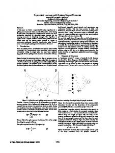
Figure 1: An ARTMAP neural network architecture specialized for pattern classification [22].
2. Supervised Training of Fuzzy ARTMAP 2.1 The Fuzzy ARTMAP Neural Network ARTMAP refers to a family of neural network architectures based on Adaptive Resonance Theory (ART) [4] that is capable of fast, stable, on-line, unsupervised or supervised, incremental learning, classification, and prediction [6, 7]. ARTMAP is often applied using the simplified version shown in Figure 1. It is obtained by combining an ART unsupervised neural network [4] with a map field. The ARTMAP architecture called fuzzy ARTMAP [7] can process both analog and binary-valued input patterns by employing fuzzy ART [5] as the ART network. The fuzzy ART neural network consists of two fully connected layers of nodes: an M node input layer, F 1 , and an N node competitive layer, F 2 . A set of real-valued weights W ={wij ∈[ 0,1]:i=1,2,... , M ; j =1,2,. .. , N } is associated with the F 1 -to- F 2 layer connections. Each F 2 node j represents a recognition category that learns a prototype vector w j =w1j ,w 2j ,... , w Mj . The F 2 layer of fuzzy ART is connected, through learned associative links, to an L node map field F ab , where L is the number of classes in the output space. A set ab ab of binary weights W ={w jk ∈[0,1]: j=1,2,... , N ;k =1,2,... , L } is associated with the F 2 -toab ab ab ab F ab connections. The vector w j =w j1 , w j2 ,... ,w jL links F 2 node j to one of the L output classes. In batch supervised training mode, ARTMAP classifiers learn an arbitrary mapping between training set patterns a =a 1 ,a 2 ,... ,a m and their corresponding binary supervision patterns t=t 1 ,t 2 , ... ,t L . These patterns are coded to have unit value t K =1 if K is the target class label for a , and zero elsewhere. Algorithm 1 describes fuzzy ARTMAP learning. Algorithm 1 Fuzzy ARTMAP learning. 1. InitializationAll the F 2 nodes are uncommitted, all weight values w ij are initialized to 1, ab and all weight values w jk are set to 0. An F 2 node becomes committed when it is selected to code an input vector a , and is then linked to an F ab node. Values of the learning rate ∈[ 0,1] , the choice 0 , the match tracking 0≪1 , and the baseline vigilance ∈[ 0,1] parameters are set. 2. Input pattern codingWhen a training pair a , t is presented to the network, a undergoes a transformation called complement coding, which doubles its number of components. The complement-coded input pattern has M =2m dimensions and is defined by 30
SUPERVISED LEARNING OF FUZZY ARTMAP NN’S THROUGH PSO A=a , a c =a1 ,a 2 ,... ,a m ; a c1 ,a c2 ,... ,a cm , where a ci =1−a i , and a i ∈[0,1 ] . The vigilance parameter is reset to its baseline value . 3. Prototype selectionPattern A activates layer F 1 and is propagated through weighted connections W to layer F 2 . Activation of each node j in the F 2 layer is determined by the Weber law choice function: T j A=
∣A∧w j∣ , ∣w j∣
(1) M
where ∣⋅∣ is the L1 norm operator defined by ∣w j∣≡∑i=1 ∣w ij∣ , ∧ is the fuzzy AND operator, A∧w j i ≡min A i ,w ij , and is the user-defined choice parameter. The F 2 layer produces a binary, winner-take-all pattern of activity y= y1 , y 2 ,... , y N such that only the node j=J with the greatest activation value J =argmax {T j : j=1,2,... , N } remains active; thus y J =1 and y j =0, j≠ J . If more than one T j is maximal, the node j with the smallest index is chosen. Node J propagates its top-down expectation, or prototype vector w J , back onto F 1 and the vigilance test is performed. This test compares the degree of match between w J and A against the dimensionless vigilance parameter ∈[ 0,1] :
∣A∧w J∣ ∣ A∧w J∣ =
∣A∣
M
≥ .
(2)
If the test is passed, then node J remains active and resonance is said to occur. Otherwise, the network inhibits the active F 2 node (i.e., T J is set to 0 until the network is presented with the next training pair a , t ) and searches for another node J that passes the vigilance test. If such a node does not exist, an uncommitted F 2 node becomes active and undergoes learning (Step 5). The depth of search attained before an uncommitted node is selected is determined by the choice parameter . 4. Class predictionPattern t is fed directly to the map field F ab , while the F 2 category y learns to activate the map field via associative weights W ab . The F ab layer produces a ab ab ab ab ab binary pattern of activity y = y1 , y 2 ,... , y L =t ∧w J in which the most active F ab node K =argmax {y ab yields the class prediction ( K =k J ). If node K k : k =1,2,... , L } constitutes an incorrect class prediction, then a match tracking signal raises the vigilance parameter just enough:
∣A∧w J∣
=
M
,
(3)
where =0 , to induce another search among F 2 nodes in Step 3. This search continues until either an uncommitted F 2 node becomes active (and learning directly ensues in Step 5), or a node J that has previously learned the correct class prediction K becomes active. 5. LearningLearning input a involves updating prototype vector w J , and, if J corresponds to a newly-committed node, creating an associative link to F ab . The prototype vector of F 2 node J is updated according to: w ' J = A∧w J 1− w J ,
(4)
where is a fixed learning rate parameter. The algorithm can be set to slow learning with 01 , or to fast learning with =1 . With complement coding and fast learning, fuzzy ARTMAP represents category j as an m -dimensional hyperrectangle R j that is just large 31
GRANGER ET AL. enough to enclose the cluster of training set patterns a to which it has been assigned. That is, an M -dimensional prototype vector w j records the largest and smallest component values of training subset patterns a assigned to category j . The vigilance test limits the growth of hyperrectangles – a close to 1 yields small hyperrectangles, while a close to 0 allows large hyperrectangles. A new association between F 2 node J and F ab node K k J =K is learned by setting w ab Jk =1 for k =K , where K is the target class label for a , and 0 otherwise. The next training subset pair a , t is presented to the network in Step 2. Batch supervised training ends in accordance with some learning strategy, following one or more epochs. An epoch is defined as one complete presentation of all the patterns of a finite training data set. Once the weights W and W ab have been found through this process, ARTMAP can predict a class label for an input pattern by performing Steps 2, 3 and 4 without any vigilance or match tests. During testing, a pattern a that activates node J is predicted to belong to class K =k J . The time complexity required to process one input pattern, during either a training or testing phase, is OMN . 2.2 Typical Batch Supervised Learning Strategies Given a large training data set, one of the following four learning strategies are typically used to select e , the total number of epochs needed to end batch supervised learning by fuzzy ARTMAP: One epoch (1EP): The learning phase ends after one epoch ( e=1 ) of the training data set. (This learning strategy is mainly used for reference during simulations.) Convergence based on training set classifications (CONVp): The learning phase ends after the epoch e for which all patterns of the training data set have ab been correctly classified by the network. Convergence occurs when ∑l t l − yl , e =0 over all patterns l in the training set. Note that this strategy is prone to convergence problems for data with overlapping class distributions, as some training patterns in the overlap region may never be correctly classified. Convergence based on weight values (CONVw): The learning phase ends after the epoch e for which the weight values have converged. Convergence occurs when the sum-squared-fractional-change (SSFC) of weights W for a e−1 e, two successive epochs, and is less than 0.001, 2 SSFC=∑ j ∑i w ji e−w ji e−1 0.001 . Hold-out validation (HV): The learning phase ends after the epoch e for which the generalization error is minimized on an independent validation subset. Learning is performed using a holdout validation technique [49], with network training halted for validation after each epoch. In practice, the number of epochs that achieves the lowest generalization error should be selected by observing several epochs after e to avoid falling into local minimums. With large data sets considered in this paper, the HV an is appropriate learning strategy. If data was limited, kfold cross-validation would be a more suitable validation strategy, at the expense of some estimation bias due to crossing.
32
SUPERVISED LEARNING OF FUZZY ARTMAP NN’S THROUGH PSO
3. Supervised Learning with Particle Swarm Optimization 3.1 Evolving neural networks According to Yao [57], the concept of evolution has been introduced into neural networks at three different levels: connection weights, architectures, and learning rules. Weight training in neural networks is usually formulated as minimization of an error function by iteratively adjusting the connection weights. Several training methods are based on gradient descent, which has been successfully applied in several domains of application. However, its drawback is that it can get trapped in a local minima of the error function. To overcome this problem, several researchers have formulated the training as the evolution of connection weights, using for that genetic algorithms [29, 55]. The first level of evolution assumes that the architecture of the network is fixed, i.e., that the network topology is pre-defined and does not change during the evolution of connection weights. However, architecture design is crucial for neural networks since it has a significant impact on the generalization capabilities of a neural network. In light of this, several authors have formulated the design of the architecture as a search problem [41, 55]. One major problem with the evolution of architectures without connection weights is noise fitness evaluation [58]. In other words, the evolution of the connection weights depends on the architecture. This has led researchers to develop approaches where architectures and connection weights evolve simultaneously [34, 39, 59]. Finally, the last level takes into account the evolution of user-defined hyper-parameter values and the weight learning rule. The first attempts in this level considered the adjustment of some parameters of the backpropagation algorithm, such as learning rate and momentum [32]. Harp et al. proposed the simultaneous evolution of both hyper-parameters and architecture [28]. The idea is that it facilitates exploration of interactions between the learning algorithm and architectures such that a near-optimal combination of the parameters with an architecture can be found. As one could observe, most of the approaches reviewed here exploit genetic algorithms or other evolutionary strategies to evolve a neural network. After the development of Particle Swarm Optimization in 1995 [30], several comparisons between genetic algorithms and PSO have been published in literature [16, 26, 48]. Most of them point out the advantages of PSO over genetic algorithms, and stress the fact that the basic PSO algorithm is quite simple and easy to understand. Based on all these, researchers have applied PSO to evolve neural networks at all the aforementioned levels with considerable success [13, 23, 24, 60]. However, to the best of our knowledge, no research has been published on evolving Fuzzy ARTMAP with PSO. The rest of this section introduces an alternative to typical learning strategies – called the PSO learning strategy – for batch supervised learning of fuzzy ARTMAP neural networks. It is based on PSO, and allows to optimize weight and hyper-parameter values such that the network’s generalization error is minimized. The architecture, weights, and parameters are in effect selected to minimize generalization error by virtue of ARTMAP training, which allows to grow the network architecture (i.e., the number of F 2 nodes) based on the complexity of the problem. 3.2 The PSO learning strategy PSO is a population-based stochastic optimization technique that was inspired by social behavior of bird flocking or fish schooling [30]. It shares many similarities with evolutionary computation techniques such as genetic algorithms (GAs), yet has no evolution operators such as crossover and mutation. PSO belongs to the class of evolutionary algorithm techniques that does not utilize the “survival of the fittest” concept, nor a direct selection function. A solution with lower fitness values can therefore survive during the optimization and potentially visit any point of the search 33
GRANGER ET AL.
y
sq+1
vq+1 vq
pgq
Global Best (gBest)
q
pi
sq
Particle's Best (pBest)
x Figure 2: PSO update of a particle’s position s q to s q1 in a 2-dimensional space during iteration q1 .
space [16]. Finally, while GAs were conceived to deal with binary coding, PSO was designed, and proved very effective, in solving real valued global optimization problems, which makes it suitable for this large scale study. With PSO, each particle corresponds to a single solution in the search space, and the population of particles is called a swarm. All particles are assigned position values which are evaluated according to the fitness function being optimized, and velocities values which direct their movement. Particles move through the search space by following the particles with the best fitness. Assuming a d-dimensional search space, the position of particle i in an P-particle swarm is represented by a d-dimensional vector si =si1 , si2 ,... , sid , for i=1,2,... , P . The velocity of this particle is denoted by vector v i =v i1 , v i2 ,... ,v id , while the best previously-visited position of this particle is denoted as pi = p i1 , p i2 ,... , pid . For each new iteration q1 , the velocity and position of particle i are updated according to: v q1 =wq v qi c 1 r 1 p qi −sqi c2 r 2 pqg −sqi i
(5)
sq1 =sqi v iq1 i
(6)
where p g represents the global best particle position in the swarm, w q is the particle inertia weight, c 1 and c 2 are two positive constants called cognitive and social parameters, respectively, and r 1 and r 2 are random numbers uniformly distributed in the range [0,1] . The role of w q in Equation 5 is to regulate the trade-off between exploration and exploitation. A large inertia weight facilitates global search (exploration), while a small one tends to facilitate fine-tuning the current search area (exploitation). This is why inertia weight values are defined by some monotonically decreasing function of q . Proper fine-tuning of c 1 and c 2 may result in faster convergence of the algorithm and alleviation of the local minima. Kennedy and Eberhart propose that the cognitive and social scaling parameters be selected such that c 1 =c 2 =2 [31]. Finally, the parameters r 1 and r 2 are used to maintain the diversity of the q q1 population. Figure 2 depicts the update by PSO of a particle’s position from si to si . Algorithm 2 shows the pseudo-code of the PSO learning strategy applied to supervised training of fuzzy ARTMAP neural networks. It seeks to minimize fuzzy ARTMAP generalization q error E si in the 4-dimensional space of user-defined hyper-parameter values, q q q si =i ,i , qi ,qi . Measurement of any fitness values E sqi in this algorithm involves computing the generalization error on a validation subset for the fuzzy ARTMAP network which 34
SUPERVISED LEARNING OF FUZZY ARTMAP NN’S THROUGH PSO q has been learned using a training subset and using the parameter values at particle position si . q q When selecting pi or p g , if the two fitness values being compared are equal, then the particle requiring fewer resources. Following the last iteration of Algorithm 2, overall generalization q error is computed on a test set for the network corresponding to particle position p g . For enhanced computational throughput and global search capabilities, Algorithm 2 is inspired by the synchronous parallel version of PSO [47]. It utilizes a basic type of neighborhood called global best or gbest, which is based on a sociometric principle that conceptually connects all the members of the swarm to one another. Accordingly, each particle is influenced by the very best performance of any member of the entire swarm. Exchange of information only takes place q among the particle’s own experience (the location of its personal best pi , lbest), and the q experience of the best particle in the swarm (the location of the global best p g , gbest), instead of being carried from fitness dependent selected parents to descendants as in GAs. Note that this strategy is somewhat similar to HV in that a validation subset is used to converge on the best solutions. At the same time, any one of the typical learning strategies (1EP, CONVp, CONVw, HV) may be embedded into the PSO strategy, to train fuzzy ARTMAP based q on si . If the HV strategy is embedded, the same validation subset can be used to select the number of epochs the minimizes generalization error as to compute fitness values. The basic PSO learning strategy is equivalent to embedding 1EP.
Algorithm 2 PSO Learning Strategy for Fuzzy ARTMAP. A. InitializationSelect the internal learning strategy: 1EP, CONVp, CONVw or HV Set the maximum number of iteration q max and/or fitness objective E∗ Set PSO parameters P , vmax , w 0 , c 1 , c 2 , r 1 and r 2 0 0 d Initialize particle positions at random such that si and pi ∈[0,1] , for i=1,2,... , P 0 Initialize particle velocities at random such that 0≤v i ≤v max , for i=1,2,... , P
B. Iterative processSet iteration counter q=0 q ∗ while q≤q max or E p g ≥E do
for i=1,2,. .. , P do q Train fuzzy ARTMAP according to internal learning strategy, using si q Compute fitness value E si of resulting network q q q q if E si E pi then Update particle’s best personal position: pi =si
end q Select the particle with best global fitness: g=argmin {E si :i=1,2,... P }
for i=1,2,... , P do q1 q q q q q q Update velocity: v i =w v i c 1 r 1 p i −si c2 r 2 p g −si q1 q q1 Update position: si =si v i
end q=q1
Update particle inertia w q end
35
GRANGER ET AL.
4. Experimental Methodology In order to observe the influence on fuzzy ARTMAP performance of data set manipulations and parameter settings from a perspective of different data structures, several data sets were selected for computer simulations. Four synthetic data sets are representative of pattern recognition problems that involve either (1) simple decision boundaries with overlapping class distributions, or (2) complex decision boundaries, were class distributions do not overlap on decision boundaries. A set of handwritten numerical characters from the NIST SD19 database is representative of complex real-world pattern recognition problems. Prior to a simulation trial, these data sets were normalized according to the minmax technique [45], and partitioned into three parts – the training subset, the validation subset, and the test subset. Previous results have shown that no significant differences in performance were achieved by fuzzy ARTMAP as a result of using the Gaussian normalization technique on the same synthetic data sets as this paper [27]. In addition, Gaussian normalization is not applicable to the NIST SD19 data, as the features extracted from isolated numbers have multi-modal distribution, and some modes are not Gaussian. During each simulation trial, the performance of fuzzy ARTMAP is compared from a perspective of different training subset size, learning strategies, and parameter settings. In order to assess the effect on performance of training subset size, the number of training subset patterns used for supervised learning was progressively increased, while corresponding validation and test subsets were held fixed. To assess the impact of typical learning strategies, the performance was compared for fuzzy ARTMAP neural networks where supervised learning was ended (1) after one complete epoch (1EP), (2) once no training set patterns are misclassified during an epoch (CONVp), (3) once weight values remain constant for two successive epochs (CONVw), and (4) once performance is maximized on a validation set, through holdout validation based on the number of epochs (HV). In either case, the number of epochs was limited to 1000, and pattern presentation orders were always randomized from one epoch to the next. Since the HV strategy does not suffer from overtraining due to the number of training epochs, the impact of the number of training epochs on performance may also be assessed. Finally, to assess the impact of hyperparameter settings, fuzzy ARTMAP performance was first measured when using parameter settings that yield minimum network resources (internal categories, epochs, etc.): =1 , =0.001 , =0 , and either =−0.001 or =0.001 . It is worth noting that a convergence problem occurs when learning inconsistent cases, whenever the training subset contains identical patterns that belong to different classes. The consequence is a failure to converge, as identical prototypes linked to inconsistent cases proliferate. This problem may be circumvented by using the feature of ARTMAP-IC [11] called negative match tracking (denoted MT-), with ≤0 . Both the original MT+ ( =0.001 ) and MT( =−0.001 ) were considered during simulations. Then, performance was compared to fuzzy ARTMAP using the PSO learning strategy, when parameter values were selected to minimize generalization error. In all simulations involving the PSO learning strategy, the 4-dimensional search space was set to the following range of fuzzy ARTMAP hyper-parameters: ∈[ 0,1] , ∈[0.00001,1 ] , ∈[ 0,1] , and ∈[−1,1 ] . Each simulation trial was performed with P=15 particles, and ended after q max =100 iterations (although none of our simulations has ever attained this limit). A q fitness objective E∗ was not considered to end training, but a trial was also ended if E p g is constant for 10 consecutive iterations. All but one of the particle vectors were initialized 0 randomly, according to a uniform distribution in the search space. The initial position s1 of one particle was set with the hyper-parameters that yield minimum resources ( =1 , =0.001 , 36
SUPERVISED LEARNING OF FUZZY ARTMAP NN’S THROUGH PSO =0 , and =0.001 ). During preliminary simulations with the PSO strategy, the authors have observed very little sensitivity of results to fuzzy ARTMAP’s initial parameter values. However, restraining the PSO search space to useful ranges of parameter values limits the resource (number of PSO iterations and number of particles) needed to minimize PSO’s cost function. The PSO parameters were set as follows: c 1 =c 2 =2 ; r 1 and r 2 were random numbers uniformly distributed in [0,1]; w q was decreased linearly from 0.9 to 0.4 over the q max iterations; the components of v max were set to 0.1 for , , and , and to 0.2 for . At the end of a trial, q the fuzzy ARTMAP network with the best global fitness value p g was retained. Independently trials were repeated 4 times with different initializations of particle vectors, and the network with q greatest p g of the four was retained. From previous study with our data sets, it was determined that performing 4 independent trials of the PSO learning strategy with only 15 particles leads to better optimization results than performing 1 trial with 60 particles. Since fuzzy ARTMAP performance is sensitive to the presentation order of the training data, each simulation trial was repeated 10 times with either 10 different randomly generated data sets (synthetic data), or 10 different randomly selected data presentation orders (NIST SD19 data). The average performance of fuzzy ARTMAP was assessed in terms of resources required during training, and its generalization error on the test sets. The amount of resources required during training is measured by compression and convergence time. Compression refers to the average number of training patterns per category prototype created in the F 2 layer. Convergence time is the number of epochs required to complete learning for a learning strategy. It does not include presentations of the validation subset used to perform hold-out validation. Generalization error is estimated as the ratio of incorrectly classified test subset patterns over all test set patterns. Given that compression indicates the number of F 2 nodes, the combination of compression and convergence time provides useful insight into the amount of processing required by fuzzy ARTMAP during training to produce its best asymptotic generalization error. Average results, with corresponding standard error, are always obtained, as a result of the 10 independent simulation trials. The Quadratic Bayes and k-Nearest-Neighbor with Euclidean distance (k-NN) classifiers were included for reference with generalization error results. These are classic parametric and non-parametric classification techniques from statistical pattern recognition, which are immune to the effects of overtraining. For each computer simulation, the value of k employed with k-NN was selected among k = 1, 3, 5, 7, and 9, using hold-out validation. The rest of this section gives some additional details on the synthetic and real data sets and data normalization technique employed during computer simulations.
4.1 Synthetic data sets All four synthetic data sets described below are composed of a total of 30,000 randomlygenerated patterns, with 10,000 patterns for the training, validation, and test subsets. They correspond to 2 class problems, with a 2 dimensional input feature space. Each data subset is composed of an equal number of 5,000 patterns per class. In addition, the area occupied by each class is equal. During simulation trials, the number of training subset patterns used for supervised learning was progressively increased from 10 to 10,000 patterns according to a logarithmic rule: 5, 6, 8, 10, 12, 16, 20, 26, 33, 42, 54, 68, 87, 110, 140, 178, 226, 286, 363, 461, 586, 743, 943, 1197, 1519, 1928, 2446, 3105, 3940, 5000 patterns per class. This corresponds to 30 different simulation trials over the entire 10,000 pattern training subset. The four synthetic data sets have been selected to facilitate the observation of fuzzy ARTMAP behavior on different tractable problems. Of the four sets, two have simple linear decision boundaries with overlapping class distributions, D tot and D tot , and two have 37
GRANGER ET AL.
(b) Dσ (ξtot )
(a) Dµ (ξtot )
(d) DP2
(c) DCIS
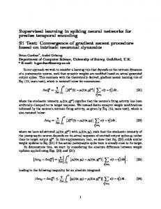
Figure 3: Representation of the synthetic data sets used for computer simulations.
complex non-linear decision boundaries without overlap, DCIS and D P2 . The total theoretical probability of error associated with D and D is denoted by tot . Note that with D CIS and D P2 , the length of decision boundaries between class distributions is longer, and fewer training patterns are available in the neighborhood of these boundaries than with D tot and D tot . In addition, note that the total theoretical probability of error with D CIS and D P2 is 0, since class distributions do not overlap on decision boundaries. The four synthetic data sets are now described: D tot : As represented in Figure 3(a), this data consists of two classes, each one defined by a multivariate normal distribution in a two dimensional input feature space. It is assumed that data is randomly generated by sources with the same Gaussian noise. Both sources are 2 described by variables that are independent and have equal variance , therefore distributions are hyperspherical. In fact, D tot refers to 13 data sets, where the degree of overlap, and thus the total probability of error between classes differs for each set. The degree of overlap is varied from a total probability of error, tot =1% to tot =25% , with
38
SUPERVISED LEARNING OF FUZZY ARTMAP NN’S THROUGH PSO 2% increments, by adjusting the mean vector 2 of class 2. The reader is referred to Table 3 (Appendix A) for the specific parameters employed to create the 13 data sets of D tot . D tot : As represented in Figure 3(b), this data is identical to D tot , except that the degree 2 of overlap between classes is varied by adjusting the variance 2 of both classes. The parameters employed to create the 13 data sets of D tot are presented in Table 4 (Appendix A). Note that for a same degree of overlap, D tot data sets have a larger overlap boundary than D tot yet they are not as dense. D CIS : As represented in Figure 3(c), the Circle-in-Square problem [6] requires a classifier to identify the points of a square that lie inside a circle, and those that lie outside a circle. The circle’s area equals half of the square. It consists of one non-linear decision boundary where classes do not overlap. D P2 : As represented in Figure 3(d), each decision region of the D P2 problem is delimited by one or more of the four following polynomial and trigonometric functions: f 1 x =2 sin x 5
(7)
f 2 x = x−22 1
(8)
f 3 x =−0.1 x 2 0.6 sin 4 x 8
(9)
f 4 x =0.5 x −102 7.902
(10)
and belongs to one of the two classes, indicated by the Roman numbers I and II [51]. It consists of four non-linear boundaries, and class definitions do not overlap. Note that equation f 4 x was slightly modified from the original equation such that the area occupied by each class is approximately equal. 4.2 NIST Special Database 19 The NIST Special Database 19 (SD19) [25] data set has been selected due to the great variability and difficulty of such handwriting recognition problems (see Figure 4). It consists of images of
Figure 4: Some images of handwritten digits extracted from the NIST SD19 data set.
39
GRANGER ET AL. handwritten sample forms (hsf) organized into eight series, hsf-{0,1,2,3,4,6,7,8}. SD19 is divided in 3 sections which contains samples representing isolated handwritten digits (’0’, ’1’, ..., ’9’) extracted from hsf-{0123}, hsf-7 and hsf-4. Table 5 (Appendix A) shows the distribution of samples among the 10 digit classes according to this division. For our simulations, the data in hsf-{0123} has been further divided into training subset (150,000 samples), validation subset 1 (15,000 samples), validation subset 2 (15,000 samples) and validation subset 3 (15,000 samples). The training and validation subsets contain an equal number of samples per class. Data in hsf-7 and hsf-4 have been used as a standard test subset (all 60,089 samples) and a noisy test subset (all 58,647 samples), respectively. The distribution of samples per class in test sets is approximately equal. The set features extracted for samples is a mixture of concavity, contour, and surface characteristics [42]. Accordingly, 78 features are used to describe concavity, 48 features are used to describe contour, and 6 features are used to describe surface. Each sample is therefore composed of 132 features that are normalized between 0 and 1 by summing up their respective feature values, and then dividing each one by its summation. With this feature set, the NIST SD19 data base exhibits complex decision boundaries, with moderate overlap between digit classes. Table 2 reports some experimental results obtained with Multi-Layer Perceptron (MLP), Support Vector Machine (SVM), and k-NN classifiers. During simulations, the number of training subset patterns used for supervised learning was progressively increased as from 100 to 150,000 patterns, according to a logarithmic rule. The 16 different training subset consist of the first 10, 16, 28, 47, 80, 136, 229, 387, 652, 1100, 1856, 3129, 5276, 8896, and all 15000 patterns per class.
5. Impact of Data Set Manipulations with Synthetic Data Figures 5-7 show the average performance achieved by fuzzy ARTMAP as a function of the training subset size for D tot =9 % . The error bars on these and other figures are standard error of the sample mean. Parameter values were set to minimize resources, with =0 , =1 , =0.001 and either =0.001 (MT+) or =−0.001 (MT-). These results are shown for the 1EP, CONVw, CONVp, and HV learning strategies. The generalization errors for the Quadratic Bayes and k-NN classifiers, as well as the theoretical probability of error ( tot ), are also shown for reference. ε theorical
26
QBC
24
k−NN
Estimate of Generalization Error (%)
FAM 1EP w/ MT+ FAM CONVp w/ MT+
22
FAM CONVw w/ MT+ FAM HV w/ MT+
20 FAM HV w/ MT−
18
16
14
12
10
1
10
2
10 Number of Training Patterns per Class
3
10
Figure 5: Average generalization error of fuzzy ARTMAP (with the 1EP, CONVw, CONVp, and HV) versus training subset size for D tot =9% using =1 , =0.001 , =0 , and =±0.001 .
40
SUPERVISED LEARNING OF FUZZY ARTMAP NN’S THROUGH PSO 45 1
FAM 1EP w/ MT+ FAM CONVp w/ MT+ FAM CONVw w/ MT+ FAM HV w/ MT+ FAM HV w/ MT−
10
FAM 1EP w/ MT+ FAM CONVp w/ MT+ FAM CONVw w/ MT+ FAM HV w/ MT+ FAM HV w/ MT−
35 Convergence Time (Number of Epochs)
Compression (Number Training Tatterns per F2 Node)
40
30
25
20
15
10
5
0
0
1
10
2
10 Number of Training Patterns per Class
10
3
Figure 6: Average compression of fuzzy ARTMAP (with the 1EP, CONVw, CONVp, and HV) versus training subset size for D tot =9% using =1 , =0.001 , =0 , and =±0.001 .
1
10
10
2
10 Number of Training Patterns per Class
3
10
Figure 7: Average convergence time of fuzzy ARTMAP (with the 1EP, CONVw, CONVp, and HV) versus training subset size for D tot =9% using =1 , =0.001 , =0 , and =±0.001 .
These results on these figures clearly show the impact on performance of the number of epochs and of the training subset size. Fuzzy ARTMAP achieves a slightly lower average generalization error if it is trained with HV (using MT+ or MT-) rather than with CONVw or CONVp. The lowest average generalization error (about 12%) is achieved when training fuzzy ARTMAP with HV (MT+) and 10 training patterns per class. In this case, compression is on average about 6.5 patterns per F 2 node, amounting to about 3.1 F 2 nodes total, and an average convergence time of about 1 epoch. This advantage over CONVw and CONVp tends to diminish as the training set size grows. In addition, HV yields an average compression and convergence time between that obtained by 1EP and by CONVw or CONVp learning strategies. Since the HV strategy is immune to the effects of overtraining from the number of epochs, the relatively higher generalization error and lower compression obtained with CONVw and CONVp are an indication that these learning strategies can in fact lead to overtraining based on the number of epochs. The larger the training data set, the lower the impact of overtraining due to the number of training epochs. However, beyond a training set size of as little as 40 patterns per class, significant degradation in performance occurs, regardless of the learning strategy – the compression tends to stabilize or decrease, while the generalization error and convergence time tend to increase significantly. (Compression and convergence time do not degrade for 1EP.) Although the compression and convergence time does not degrade as sharply when fuzzy ARTMAP uses MT-, generalization error grows progressively beyond 20% with the training set size. Meanwhile, the generalization error of reference classifiers tend asymptotically towards their minimum value. Fuzzy ARTMAP’s behavior highlights the significant effect of overtraining related to the training set size. For data with overlapping class distributions, increasing the amount of training data beyond a certain point requires significantly more resources, while yielding a higher generalization error. Very similar tendencies are found in simulation results where fuzzy ARTMAP is trained using the other D tot and D tot data sets. However, as tot increases, the performance degradation due to training subset size tends to become more pronounced, and occurs for fewer training set patterns. As a result, the generalization error attained by fuzzy ARTMAP on these data sets may only approach those obtained by reference classifiers for very small training subset. 41
GRANGER ET AL. 16
35
FAM 1EP w/ MT+
k−NN FAM 1EP w/ MT+ FAM CONVp w/ MT+ FAM CONVw w/ MT+ FAM HV w/ MT+ FAM HV w/ MT−
FAM CONVp w/ MT+ FAM CONVw w/ MT+
30
FAM HV w/ MT+ FAM HV w/ MT−
12
Estimate of Generalization Error (%)
Overtraining Error from the Training Set Size (%)
14
FAM w/ PSO(1EP)
10
8
6
4
2
20
15
10
5
0
0
0
5
10
15 Degree of Overlap
20
25
Figure 8: Average overtraining error from the training set size as a function tot on all D tot data sets, using =1 , =0.001 , =0 , and =±0.001 .
200
1
10
2
10 Number of Training Patterns per Class
3
10
Figure 9: Average generalization error of fuzzy ARTMAP (with the 1EP, CONVw, CONVp, and HV strategies) versus training subset size for D CIS using =1 , =0.001 , =0 , and =±0.001 . FAM 1EP w/ MT+ FAM CONVp w/ MT+ FAM CONVw w/ MT+ FAM HV w/ MT+ FAM HV w/ MT−
FAM 1EP w/ MT+ FAM CONVp w/ MT+ FAM CONVw w/ MT+ FAM HV w/ MT+ FAM HV w/ MT− 1
10 Convergence Time (Number of Epochs)
Compression (Number Training Tatterns per F2 Node)
25
150
100
50
0
0
1
10
2
10 Number of Training Patterns per Class
10
3
10
1
10
2
10 Number of Training Patterns per Class
3
10
Figure 10: Average compression of fuzzy ARTMAP (with Figure 11: Average convergence time of fuzzy ARTMAP the 1EP, CONVw, CONVp, and HV strategies) versus (with the 1EP, CONVw, CONVp, and HV) versus training training subset size for D CIS using =1 , =0.001 , subset size for DCIS using =1 , =0.001 , =0 , and =0 , and =±0.001 . =±0.001 .
Recall that in this paper, HV has been applied such that training is halted based on validation after each training epoch. This eliminates the generalization error due to overtraining caused by the number of training epochs. Note that applying HV within epochs (by halting network training for fewer patterns than in one epoch) could reduce overtraining from training set size, but the computational overhead would become very costly. Let us define the overtraining error from training subset size as the difference between the maximum generalization error obtained by using all the training data (5,000 patterns per class) and the minimum generalization error obtained for some training subset size. Figure 8 displays the average trial-by-trial overtraining error from the training subset size for D tot as a function of tot for the 1EP, CONVw, CONVp, and HV strategies. For instance, with the D tot =9 % data set, the size of the training subset increases generalization error by about 4.5% for CONVp. The impact of training subset size on generalization error grows with tot , and is about twice as great for HV with Mtas with MT+.
42
SUPERVISED LEARNING OF FUZZY ARTMAP NN’S THROUGH PSO Figures 9-11 present the average performance achieved by fuzzy ARTMAP as a function of the training subset size for DCIS . Here again, parameter values were set to minimize resources, with =0 , =1 , =0.001 and either =0.001 (MT+) or =−0.001 (MT-). These results are displayed for the 1EP, CONVw, CONVp, and HV learning strategies. The generalization error for the k-NN classifier is also shown for reference. For segmented data sets with complex decision bounds like D CIS and D P2 , k-NN generally has the lowest generalization error when k =1 . The tot =0 % with DCIS and D P2 . A degradation of performance indicative of the effects of overtraining are not apparent from results on these figures. As would be expected, when training set size increases, the compression and convergence time also increase. Meanwhile, the generalization error of fuzzy ARTMAP decreases asymptotically towards its minimum. Results are comparable for CONVw, CONVp, and HV learning strategies. The best average generalization error on DCIS (about 2%) is achieved when training fuzzy ARTMAP with CONVw, CONVp, or HV and 5,000 training patterns per class. In this case, compression is about 100 patterns per F 2 node, and convergence time ranges from 8 (CONVw) to 16 (CONVp) epochs. Similar tendencies are found in simulation results where fuzzy ARTMAP is trained using the D P2 data set. However, since the decision boundaries are more complex with D P2 , a greater number of training patterns are required for fuzzy ARTMAP to asymptotically start reaching its minimum generalization error. The best average generalization error on DP2 (about 4%) is
(a) HV and MT+ (20 patterns).
(b) HV and MT+ (10,000 patterns).
(c) HV and MT- (10,000 patterns).
(d) PSO(1EP) (10,000 patterns).
Figure 12: An Example of decision boundaries formed by fuzzy ARTMAP in the input space. Training is performed (a) with HV and MT+ on the first 10 training patterns per class (for the lowest generalization error), (b) with HV and MT+ on 5,000 training patterns per class, (c) with HV and MT- on 5,000 training patterns per class, and (d) with PSO(1EP) on 5,000 training patterns per class and parameters =0.47 , =0.77 , =0.45 and =−0.56 . The optimal decision boundary for D tot =9% is also shown for reference. Note that virtually no training, validation or test subset patterns are located in the upper-left and lower-right corners of these figures
43
GRANGER ET AL. achieved when training fuzzy ARTMAP with CONVw, CONVp, or HV and 5,000 training patterns per class. In this case, compression is about 45 patterns per F 2 node, and convergence time is from about 8 to 10 epochs. Although the generalization error of fuzzy ARTMAP on DCIS and D P2 data sets is never lower that of reference classifiers, their behavior is similar. One can conclude from these results that overtraining in fuzzy ARTMAP is linked to its sequential learning of training patterns from overlapping class distributions. Figure 12(a) and (b) present an example of a decision boundary obtained when fuzzy ARTMAP with MT+ is trained through HV on 20 and then on 10,000 training patterns of the D tot =9 % data set, respectively. Figure 12(a) corresponds to lowest generalization error of about 12% using 3 F 2 nodes, while Figure 12(b) corresponds to generalization error of about 15% using 916 F 2 nodes. Figure 12(c) presents a decision boundary obtained when fuzzy ARTMAP with MT- is trained through HV on 10,000 training patterns. It corresponds to generalization error of about 21%, but uses only using 199 F 2 nodes. In an attempt to learn overlapping class distributions, fuzzy ARTMAP with MT+ or MT- tends to create a growing number of small category hyperrectangles, which leads to granular decision boundaries. However, as the number of training patterns increases, the amount of resources needed to learn overlapping data grows, and generally produces poor generalization. Although HV is commonly-used to avoid overtraining, it does not appear justified given the resulting level of performance in the present experiments. It does not prevent overtraining from the training set size, and involves a considerable computational cost. To minimize generalization error, a training set size would need to be selected. Overtraining is not an issue for data from non-overlapping class distribution, even when complex decision boundaries must be formed. Performance tends to either increase or remain stable with a growing amount of training data.
6. Impact of Parameter Settings with Synthetic Data Figures 13-15 show an example of the average performance achieved by fuzzy ARTMAP with the PSO learning strategy as a function of the training subset size for D tot =9 % . Error bars are standard error of the sample mean. These results are shown for the cases where 1EP, CONVw, CONVp, and HV are embedded into the PSO strategy as internal learning strategies (to q compute the E si values). The performance of fuzzy ARTMAP with HV learning strategy and MT+ is reproduced from Figure 5 for comparison. The generalization errors for the Quadratic Bayes and k-NN classifiers, as well as the theoretical probability of error ( tot ), are also shown 22 ε theorical QBC k−NN FAM w/ PSO(1EP) FAM w/ PSO(CONVp) FAM w/ PSO(CONVw) FAM w/ PSO(HV) FAM HV w/ MT+
Estimate of Generalization Error (%)
20
18
16
14
12
10
1
10
2
10 Number of Training Patterns per Class
3
10
Figure 13: Average generalization error of fuzzy ARTMAP (with the PSO strategy) versus training subset size for D tot =9% .
44
SUPERVISED LEARNING OF FUZZY ARTMAP NN’S THROUGH PSO
5
10
3
10
Convergence Time (Number of Epochs)
Compression (Number Training Tatterns per F2 Node)
6
10
FAM w/ PSO(1EP) FAM w/ PSO(CONVp) FAM w/ PSO(CONVw) FAM w/ PSO(HV) FAM HV w/ MT+
2
10
4
10
3
10
FAM w/ PSO(1EP) 2
10
FAM w/ PSO(CONVp) FAM w/ PSO(CONVw) FAM w/ PSO(HV)
1
1
10
10
FAM HV w/ MT+
0
1
10
2
10 Number of Training Patterns per Class
10
3
10
1
10
2
10 Number of Training Patterns per Class
3
10
Figure 14: Average compression of fuzzy ARTMAP (with Figure 15: Average convergence time of fuzzy ARTMAP the PSO strategy) versus training subset size for (with the PSO strategy) versus training subset size for D tot =9% . D tot =9% .
for reference. Very similar tendencies are found in simulation results where fuzzy ARTMAP is trained using the other D tot and D tot data sets. The results shown in Figure 13 indicate that the PSO learning strategy produces a generalization error which is just above the theoretical probability of error (9%), and which is always lower than or comparable to that of reference classifiers. A generalization error of between 9% and 10% is achieved regardless learning strategy used to compute fitness (1EP, CONVw, CONVp or HV), thus the number of epochs, and of the training subset size. Therefore, the PSO strategy allows to efficiently learn data from very small and very large training subsets. Compared to the HV learning strategy alone, the generalization error is reduced by a rate of about 25% to 45% depending on the training subset size. The low generalization is accompanied by a very high level of compression that tends to grow exponentially with the number of training patterns. For example, when the training subset contains 1000 patterns per class, the compression obtained with the PSO strategy with 1EP is about 900 patterns per F 2 node. This amounts to about 2.2 F 2 nodes total. In this case, compression with PSO(1EP) is about 25 times greater than that of the HV learning strategy with MT+ alone. To minimize generalization error, the PSO strategy selects parameters that limit the number of small category hyper-rectangles created to define areas with overlapping decision bounds. As an example, Figure 12(d) presents a decision boundary obtained when fuzzy ARTMAP is trained using the PSO strategy on 10,000 training patterns D tot =9 % . It corresponds to generalization error of about 9% using only 2 F 2 nodes. Improvements to generalization error and compression are produced at the expense of a longer convergence time. In the best-case scenario, the PSO strategy with 1EP requires a maximum convergence time of 6000 epochs (100 iterations × 4 independent trials × 15 particles) assuming that validation subset presentations are not counted. When CONVw, CONVp or HV are embedded, this time is multiplied by the usual number of epochs each one needs to end batch supervised training (when computing fitness values). However, there is no clear advantage to q embedding the CONVw, CONVp or HV as internal learning strategies to compute E si values. Parameter optimization appears to compensate for the single training epoch of PSO(1EP). Overall, the PSO learning strategy leads to a very high level of performance, and eliminates the effects of overtraining for data with overlapping class distributions. Regardless of the tot value, increasing the training subset size or the number of training epochs never degrades fuzzy
45
GRANGER ET AL. 35
k−NN FAM w/ PSO(1EP) FAM w/ PSO(CONVp) FAM w/ PSO(CONVw) FAM w/ PSO(HV) FAM HV w/ MT+
Estimate of Generalization Error (%)
30
25
20
15
10
5
0
1
2
10
3
10 Number of Training Patterns per Class
10
Figures 16: Average generalization error of fuzzy ARTMAP (with the PSO strategy) for D CIS .
2
FAM w/ PSO(1EP) FAM w/ PSO(CONVp) FAM w/ PSO(CONVw) FAM w/ PSO(HV) FAM HV w/ MT+
4
10 Convergence Time (Number of Epochs)
Compression (Number Training Tatterns per F2 Node)
10
1
10
3
10
FAM w/ PSO(1EP) 2
10
FAM w/ PSO(CONVp) FAM w/ PSO(CONVw) FAM w/ PSO(HV) FAM HV w/ MT+
1
10
0
10 1
10
2
10 Number of Training Patterns per Class
1
10
3
10
2
10 Number of Training Patterns per Class
3
10
Figure 17: Average compression of fuzzy ARTMAP (with Figure 18: Average convergence time of fuzzy ARTMAP the PSO strategy) for D CIS . (with the PSO strategy) for D CIS .
ARTMAP’s generalization error or compression (refer to Figure 8). As shown in Figures 23-26 (Appendix C), simulation results are obtained with fuzzy ARTMAP parameters that vary significantly for different training subset sizes and number of epochs. Nonetheless, the hyperparameters found through the PSO strategy remain on average in the following ranges: ∈[ 0.3 ,0.55 ] , ∈[ 0.6,0 .9] , ∈[0.35, 0.7 ] and ∈[−0.65,−0.2] , which differs considerably from those employed in Section 5. Note that using negative values is an important factor in limiting the excessive creation of categories to represent areas with overlapping decision bounds. Figures 16-18 present the average performance achieved by fuzzy ARTMAP with the PSO strategy as a function of the training subset size for DCIS . These results are shown for the cases where 1EP, CONVw, CONVp, and HV learning strategies are embedded into the PSO strategy. The performance of fuzzy ARTMAP with HV learning strategy and MT+ is reproduced from Figures 9-11 for comparison. In addition, the generalization errors for the k-NN classifier is also shown for reference. Recall that tot =0 % with DCIS and D P2 . Similar tendencies are found in simulation results where fuzzy ARTMAP is trained using the D P2 data set. As shown in these figures, when the training set size increases, the generalization error of all classifiers decreases asymptotically towards their minimum. Compared to the HV learning 46
SUPERVISED LEARNING OF FUZZY ARTMAP NN’S THROUGH PSO strategy alone, the generalization error is reduced by a rate of about 40% to 60% depending on the training subset size and the internal learning strategy. For a training subset size of 100 patterns or less, the generalization error obtained using fuzzy ARTMAP with PSO strategy is significantly lower than that of k-NN. With small amounts of training patterns, embedding HV into the PSO strategy always yields the lowest generalization error. Beyond about 100 patterns per class, the generalization error using fuzzy ARTMAP with PSO strategy is comparable to that q of k-NN, regardless of the strategy used to compute E si values. The lowest average generalization error on DCIS (about 1%) is achieved when the training subset contains 5,000 patterns per class. The level of compression associated with fuzzy ARTMAP is however low, and does not tend to grow with the number of training patterns. For example, when the training subset contains 1000 patterns per class, the compression obtained using the PSO strategy with 1EP is about 3 patterns per F 2 node. This amounts to about 667 F 2 nodes total. In this specific case, compression of the HV learning strategy alone is about 16 times greater. To minimize generalization error, the PSO strategy selects parameters that encourage the creation of many small category hyper-rectangles to define areas with complex decision bounds. Indeed, the level of compression obtained when using PSO is linked to the geometry of the decision boundaries among classes. With simple boundaries, fewer large F 2 nodes are be defined, and with complex boundaries, a greater number of F 2 nodes are be defined. In the latter case, the PSO strategy can be expensive, as a training time increases with the number of F 2 nodes. The overhead in convergence time is once again several orders of magnitude greater with PSO. Furthermore, embedding CONVw, CONVp or HV into the PSO strategy requires about 2 to 10 times as many q epochs to end batch supervised learning (when computing E si values) as with respective strategies alone (see Figure 11). The PSO learning strategy globally leads to a very low generalization error for data with complex decision boundaries without overlap. The effects of overtraining are never perceived in results on Figures 16-18. In contrast, the level of compression is low and convergence time is high. With the PSO strategy, the amount of resources grow with the complexity of decision bounds that must be implicitly defined to achieve a low generalization error. As shown in Figures 30-27 (Appendix C), simulation results are obtained with fuzzy ARTMAP hyper-parameters that remain on average in the following ranges: ∈[ 0.4,1] , ∈[ 0.45,0 .95] , ∈[0.25,0 .6] and ∈[−0.5,0 .4] , which differs considerably from those in Section 5. Note that the positive values favor the creation of many small categories to define complex non-linear decision boundaries. Table 1 shows the generalization error obtained by reference classifiers and the fuzzy ARTMAP neural network using different learning strategies on some synthetic data sets. Tables 6 and 7 respectively present these results for all other D tot and D tot data sets (Appendix B). When using PSO(1EP), the generalization error of fuzzy ARTMAP is always significantly lower than when using typical learning strategies, and is even comparable to the Quadratic Bayes and k-NN classifiers on D tot and D tot data sets. Although outside the scope of this paper, the PSO strategy also appears to reduce the effect on generalization error of presentation order, as observed by the small standard error values in results. (Pattern presentation order during the learning phase of ARTMAP networks are known to have a significant impact on the network’s ability to generalize.)
47
GRANGER ET AL. 1−NN FAM 1EP w/ MT+ FAM HV w/ MT+ FAM w/ PSO(1EP)
20 18
Estimate of Generalization Error (%)
Estimate of Generalization Error (%)
16 14 12 10 8 6
1−NN FAM 1EP w/ MT+ FAM HV w/ MT+ FAM w/ PSO(1EP)
30
25
20
15
10
4 5
2 0
0
1
2
10
3
10 10 Number of Training Patterns per Class
1
4
Figure 19: Fuzzy ARTMAP generalization error versus training subset size on hsf-7 for the NIST SD19 data.
2
10
10
4
10
Figure 20: Fuzzy ARTMAP generalization error versus training subset size on hsf-4 for the NIST SD19 data.
FAM 1EP w/ MT+ FAM HV w/ MT+ FAM w/ PSO(1EP)
FAM 1EP w/ MT+ FAM HV w/ MT+ FAM w/ PSO(1EP) 2
10
Convergence Time (Number of Epochs)
Compression (Number Training Tatterns per F2 Node)
3
10 10 Number of Training Patterns per Class
2
10
1
10
1
10
0
10 1
2
10
3
10 10 Number of Training Patterns per Class
Figure 21: Average compression of fuzzy ARTMAP versus training subset size for the NIST SD19 data.
1
10
4
10
2
3
4
10 10 Number of Training Patterns per Class
10
Figure 22: Average convergence time of fuzzy ARTMAP versus training subset size for the NIST SD19 data.
Table 1: Average generalization error of reference and fuzzy ARTMAP classifiers on synthetic data sets. Training was performed on 5,000 patterns per class. Values in parenthesis are standard error of the sample mean.
Classifier
Averaged generalization error (%) D 1%
D 9 %
D 25%
D 9%
D CIS
D P2
Theoretical tot Quadratic Bayes k -NN 1-NN
1.00 9.00 25.00 9.00 0.00 1.00(0.04) 9.12(0.08) 25.11(0.10) 9.04(0.07) N/A 1.08(0.03) 9.88(0.08) 27.23(0.12) 9.66(0.07) 0.86(0.03) 1.54(0.03) 13.35(0.10) 33.49(0.17) 13.04(0.14) 0.84(0.02)
0.00 N/A 1.65(0.05) 1.61(0.04)
FAM 1EP (MT+) FAM CONVp (MT+) FAM CONVw (MT+) FAM HV (MT+) FAM HV (MT-)
2.51(0.14) 1.90(0.07) 1.97(0.09) 1.88(0.05) 2.17(0.08)
18.78(0.38) 15.44(0.15) 15.30(0.16) 15.17(0.13) 20.80(0.56)
17.98(0.29) 14.90(0.06) 14.79(0.10) 14.99(0.12) 20.13(0.43)
3.98(0.21) 1.47(0.05) 1.64(0.05) 1.58(0.05) 1.69(0.07)
7.33(0.34) 3.61(0.08) 3.66(0.08) 3.68(0.08) 4.26(0.16)
FAM PSO (1EP)
1.04(0.03)
9.35(0.08) 25.50(0.09) 9.18(0.06)
1.35(0.12)
2.05(0.10)
38.81(0.36) 36.14(0.20) 35.94(0.15) 36.10(0.20) 39.83(0.31)
48
SUPERVISED LEARNING OF FUZZY ARTMAP NN’S THROUGH PSO
7. Simulation Results with NIST SD19 Data Figures 19-22 present the average performance of fuzzy ARTMAP as a function of the training subset size for the NIST SD19 data. Error bars are standard error of the sample mean. These results are shown for the 1EP and HV learning strategies, and for the PSO strategy with 1EP used q to compute the E si values. In addition, the generalization errors for the 1-NN classifier is also shown for reference. To reduce excessive computational complexity associated with PSO on large data sets, the permissible search space for the vigilance parameter was limited to ∈[ 0,0.9] . As shown in these figures, when the training set size increases, the generalization error of all classifier tend to decrease asymptotically towards their minimum. For either hsf-7 or hsf-4, the generalization error produced by using the PSO(1EP) strategy is significantly lower than by using 1EP and HV alone. This difference tends to grow with more that 100 patterns per class. For instance, when compared to the HV strategy on the hsf-7 test subset, the PSO strategy reduces generalization error by a rate of about 25% (136 patterns per class) to 70% (15,000 patterns per class). The lowest average generalization error for hsf-7 (about 2.5%) and for hsf-4 (about 6.0%) is achieved when the training subset is close to 15,000 patterns per class. No effects of overtraining are ever observed in results with the NIST data. The level of compression for 1EP and HV strategies tend to grow exponentially with the number of training patterns. In contrast, it tends to decrease significantly beyond about 140 patterns per class with PSO(1EP). For example, when the training subset contains 1856 patterns per class, the compression obtained using the PSO(1EP) strategy is about 15 patterns per F 2 node. This amounts to about 1240 F 2 nodes in total (compared to about 100 F 2 nodes for the HV strategy). Finally, the PSO strategy requires only about 70 to 100 epochs to end batch supervised learning. With the PSO strategy, the amount of resources requirement are high due to the complexity of NIST data decision boundaries. As shown in Figures 34-31 (Appendix C), simulation results with the PSO strategy are obtained with fuzzy ARTMAP hyper-parameters that remain on average in the following ranges: ∈[ 0.1,0 .6] , ∈[ 0.75,1] , ∈[0,0.55 ] and ∈[−0.2,0 .4] , which differs considerably from those in Section 5. Recall that the NIST SD19 data base exhibits very complex decision boundaries, with moderate overlap between classes, and the positive values favor the creation of many small categories to define complex decision boundaries. Table 2 shows the generalization error obtained by the k-NN, MLP, SVM, and fuzzy ARTMAP classifiers after learning all the training data (15,000 patterns per class) of the NIST SD19 data set. When compared to the HV strategy with MT+, the PSO strategy allows to Table 2: Generalization error of different classifiers on all on the NIST SD19 data set.
Generalization error (%)
Classifier
hsf-7
hsf-4
1-NN (Euclidean distance)
1.43
3.71
Multi-Layer Perceptron [42]
0.84
2.40
SVM [38] pairwise coupling strategy SVM [38] one-against-all strategy
0.70 0.63
2.09 1.88
Fuzzy ARTMAP 1EP MT+ ( =1 , =0.001 , =0 , =0.001 ) Fuzzy ARTMAP HV MT+ ( =1 , =0.001 , =0 , =0.001 ) Fuzzy ARTMAP PSO 1EP ( =1 , =0.17 , =0.9 , =0.343 )
6.27 4.86 2.10
10.10 8.44 4.95
49
GRANGER ET AL. decreased generalization error by a rate of 41% for hsf4, and a rate of 57% for hsf7. However, with PSO(1EP), the generalization error of fuzzy ARTMAP is always significantly higher than with the other well-known reference classifiers. Even with PSO(1EP), fuzzy ARTMAP is not competitive with these classifiers due to the complex decision bounds in the data.
8. Conclusions In this paper, the impact on fuzzy ARTMAP neural network performance of practical decisions taken for batch supervised learning – data set manipulations and parameter settings – has been explored through an extensive set of computer simulations. Performance has been compared in term of generalization error and resource requirements when fuzzy ARTMAP exploits different learning strategies, training subset sizes, and parameter values. An experimental protocol has been defined such that the contribution of these decisions on performance may be isolated for synthetic and real-world pattern recognition problems that exhibit overlapping class distributions and complex decision boundaries. The results presented in this paper indicate the extent to which supervised training of fuzzy ARTMAP using typical strategies can lead to overtraining, and thus category proliferation. In particular, significant degradation in performance due to overtraining is observed for pattern recognition problems with overlapping class distributions, where fuzzy ARTMAP tends to create a growing number of small category hyper-rectangles, and defines granular decision boundaries. In this context, the overall effects of overtraining tend to increase according to the number of training epochs, and to the training set size for overlapping data. In all cases, training fuzzy ARTMAP using hold-out validation always yields a level of performance that is equal to, or higher than training it until convergence. Although the hold-out learning strategy is commonlyemployed to avoid overtraining, results indicate that the added computational complexity does not necessarily justify its use. Given that the choice of parameters may lead to overtraining, and significantly degrade the capacity to generalize, an alternative Particle Swarm Optimization (PSO) learning strategy has been introduced. It is based on the concept of neural network evolution in that it determines the set of parameters and network (weights and architecture) such that generalization error is minimized. Through a comprehensive set simulations, fuzzy ARTMAP using the PSO learning strategy has been shown to produce a significantly lower generalization error than that of fuzzy ARTMAP using typical learning strategies. Generalization error is usually above the theoretical probability of error, tot , but lower than or comparable to that of reference Quadratic Bayes and k-NN classifiers. Furthermore, the PSO learning strategy eliminates degradation of generalization error due to overtraining resulting from the number of training epochs, training set size, and data set structure. Finally, the PSO learning strategy also appears to reduce the effect on performance of pattern learning order. The lower generalization is accompanied by a high level of compression for data with overlapping decision bounds, but a low level for data with complex decision bounds. The level of compression obtained with PSO depends on the geometry of the decision boundaries among classes. To minimize generalization error, the PSO strategy selects parameters, that limits the number of category hyperrectangles created to define areas with overlapping decision bounds. In contrast, the PSO strategy selects parameters that encourage the creation of many small category hyper-rectangles to define areas with complex decision bounds. All performance improvements with the PSO strategy are achieved at the expense of a convergence time that may be orders of magnitude greater than with typical strategies alone. Fortunately, parameter optimization appears to compensate for the number of training epochs, and no advantage was found by embedding anything but the 1EP strategy inside PSO. The PSO 50
SUPERVISED LEARNING OF FUZZY ARTMAP NN’S THROUGH PSO strategy can become very costly for data sets with complex decision bounds, as a training time increases with the number of internal categories. Other variants of the PSO scheme may provide for more efficient implementations of the PSO strategy. For instance, a multi-objective PSO learning strategy, that optimizes parameters and weights based on both generalization error and compression, would yield less expensive solutions in the above case. In addition, asynchronous implementations of PSO is more efficient in problems subject to load imbalance, as processing would not halt until all particle finish one iteration before proceeding to the next iteration. Overall, results obtained with the PSO strategy highlight the importance of optimizing fuzzy ARTMAP parameters for each different problem, using a consistent objective function. In fact, the parameters found using this strategy vary significantly according to, e.g., training set size and data set structure, and differ considerably from the popular choice of parameters that minimize resources. The PSO strategy is inherently a batch learning mechanism, and as such is not entirely consistent with the ARTMAP philosophy in that parameters cannot be adapted on-the-fly, through on-line, supervised or unsupervised, incremental leaning. ARTMAP parameters should be learned progressively through some on-line gradient descent approach. Nonetheless, the PSO strategy indicates the extent to which parameter values can improve generalization error of fuzzy ARTMAP, and mitigate the performance degradation cause by overtraining. Learning large data sets where a large validation subset can be afforded for HV corresponds to having excellent prior knowledge of the problem, as this subset effectively guides the search for an optimum neural model during learning. Future work should include assessing the impact of using the PSO strategy to learn small data sets, and comparing results to the k-fold crossvalidation strategy. The impact of learning real-world, and possibly imbalanced data sets is also relevant.
Acknowledgements This research was supported in part by the Natural Sciences and Engineering Research Council of Canada.
References [1] [2]
[3] [4] [5] [6]
[7]
[8]
G. C. Anagnostopoulos, M. Georgiopoulos, S. J. Verzi, and G. L. Heileman, ”Boosted ellipsoid ARTMAP,” SPIE – Applications and Science of Comp. Intelligence V, 4739, 2002, 74-85. M. L. Bote-Lorenzo, Y. Dimitriadis, E. Gomez-Sanchez, “Automatic extraction of humanrecognizable shape and execution prototypes of handwritten characters,” Pattern Recognition, 36:7, 1605-1617, 2003. A. Canuto, G. Howells, and M. Fairhurst, “An investigation of the effects of variable vigilance within the RePART neuro-fuzzy network,” Journal of Intelligent and Robotic Systems, 29:4, 317-334, 2000. G. A. Carpenter and S. Grossberg, “A massively parallel architecture for a self-organizing neural pattern recognition machine,” Computer, Vision, Graphics and Image Processing, 37, 1987, 54-115. G. A. Carpenter, S. Grossberg, and D. B. Rosen, “Fuzzy ART: fast stable learning and categorisation of analog patterns by an adaptive resonance system,” Neural Networks, 4:6, 759-771, 1991. G.A. Carpenter, S. Grossberg, and J. H. Reynolds, “ARTMAP: supervised real-time learning and classification of nonstationary data by a self-organizing neural network,” Neural Networks, 4, 565588, 1991. G. A. Carpenter, S. Grossberg, N. Markuzon, J. H. Reynolds, and D. B. Rosen, “Fuzzy ARTMAP: a neural network architecture for incremental supervised learning of analog multidimensional maps,” IEEE Trans. on Neural Networks, 3:5, 698-713, 1992. G. A. Carpenter, S. Grossberg, and K. Iizuka, “Comparative performance measures of fuzzy ARTMAP, learned vector quantization, and back propagation for handwritten character recognition,” Proc. Int. Joint Conf. on Neural Networks, I-794-799, 1992.
51
GRANGER ET AL. [9] [10]
[11] [12] [13]
[14] [15] [16] [17] [18] [19] [20]
[21] [22] [23] [24]
[25] [26]
[27] [28] [29] [30] [31] [32]
G. A. Carpenter and W. D. Ross, “ART-EMAP: a neural network architecture for object recognition by evidence accumulation,” IEEE Trans. on Neural Networks, 6:4, 805-818, 1995 G. A. Carpenter, M. N. Gjaja, S Gopal, and C. E. Woodcock, “ART neural networks for remote sensing: vegetation classification from Landsat TM and Terrain Data,” IEEE Trans. on Geosciences and Remote Sensing, 35:2, 1997. G. A. Carpenter and N. Markuzon, “ARTMAP-IC and medical diagnosis: Instance counting and inconsistent cases,” Neural Networks, 11:2, 323-336, 1998. G. A. Carpenter, B. L. Milenova, and B. W. Noeskeand, “Distributed ARTMAP: A neural network for fast distributed supervised learning,” Neural Networks, 11, 793-813, 1998. A. Chatterjee, K. Pulasinghe, K. Watanabe, and K. Izumi, “A particle swarm optimized fuzzy-neural network for voice-controlled robot systems,” IEEE Trans. on Industrial Electronics, 52:6, 1478-1489, 2005. S. Chen, C. F. N. Cowan, and P. M. Grant, “Orthogonal least squares learning algorithm for radial basis function networks,” IEEE Trans. on Neural Networks, 2:2, 302-309, 1991. A. Dubrawski, “Stochastic validation for automated tuning of neural network’s hyper-parameters,” Robotics and Automated Systems, 21, 83-93, 1997. R. C. Eberhart and Y. Shi, “Comparison between genetic algorihms and particle swarm intelligence,” in Evolutionary Programming VII, V. W. Porto et al, eds., Springer, 611-616, 1998. P. Gamba and F. DellAcqua, “Increased accuracy multiband urban classification using a neuro-fuzzy classifier,” International Journal of Remote Sensing, 24:4, 827-834, 2003. E. Gomez-Sanchez, et. al. “Experimental study of a novel neuro-fuzzy system for on-line handwritten UNIPEN digit recognition,” Pattern Recognition Letters, 19, 357-364, 1998. E. Gomez-Sanchez, et. al. “μARTMAP: Use of mutual information for category reduction in fuzzy ARTMAP,” IEEE Trans. on Neural Networks, 13:1, 58-69, 2002. E. Granger, et. al. “A comparison of classifiers for radar emitter type identification,” in Intelligent Engineering Systems Through Artificial Neural Networks 9, Dagli, C. H. et al., eds., New York, NY: ASME Press, 3-11, 1999. E. Granger, et. al. “Classification of incomplete data using the fuzzy ARTMAP neural network,” Proc. 2000 Int. Joint Conference on Neural Networks, 4, 2000, pp. 35-40. E. Granger, et. al. “A what-and-where fusion neural network for recognition and tracking of multiple radar emitters,” Neural Networks, 14, 325-344, 2001. E. A. Grimaldi, et. al. “PSO as an effective learning algorithm for neural network applications,” in 3rd Int. Conf. on Computational Electromagnetics and Its Applications, 2004, pp. 557-560. V. G. Gudise and G. K. Venayagamoorthy, “Comparison of particle swarm intelligence and backpropagation as training algorithms for neural networks,” in IEEE Swarm Intelligence Symposium, 2003, pp. 110-117. P. J. Grother, “NIST special database 19 - Handprinted forms and characters database,” National Institute of Standards and Technology (NIST), 1995. S. J. Habib and B. S. Alkazemi, “Comparative study between the internal behavior of GA and PSO through problem-specific distance functions,” in IEEE Congress on Evolutionary Computation, 2005, pp. 2190- 2195. P. Henniges, E. Granger, and R. Sabourin, “Factors of overtraining with fuzzy ARTMAP neural networks,” Int. Joint Conference on Neural Networks, Montreal, Canada, 2005, pp. 1075-1080. S. A. Harp, T. Samad, and A. Guha, “Toward the genetic synthesis of neural networks,” 3rd Int. Conf. Genetic Algorithms and Their Applications, 1989, pp. 360-369. D. J. Janson and J. F. Frenzel, “Training product unit neural networks with genetic algorithms,” IEEE Expert, 8, 26-33, 1993. J. Kennedy and R. C. Eberhart, “Particle swarm intelligence,” Int. Conf. on Neural Network, 1995, pp. 1942-1948. J. Kennedy and R. C. Eberhart, Swarm intelligence. Morgan Kaufmann, 2001. H. B. Kim, et. al. ”Fast learning method for backpropagation neural network by evolutionary adaptation of learning rates,” Neurocomputing, 11:1, 101-106, 1996.
52
SUPERVISED LEARNING OF FUZZY ARTMAP NN’S THROUGH PSO [33] A. Koufakou, et. al. ”Cross-validation in fuzzy ARTMAP for large databases,” Neural Networks, 14, 1279-1291, 2001. [34] J. R. Koza and J. P. Rice, ”Genetic generation of both the weights and architecture for a neural network,” IEEE Int. Joint Conf. on Neural Networks, 1991, pp. 397-404. [35] C. P. Lim, H. H. Toh, and T. S. Lee, ”An evaluation of the fuzzy ARTMAP neural network using offline and on-line strategies,” Neural Network World, 4, 327-339, 1999. [36] B. Lerner and B. Vigdor, ”An empirical study of fuzzy ARTMAP applied to cytogenetics,” IEEE Convention of Electrical and Electronics Engineers in Israel, 2004, pp. 301-304. [37] S.-J. Lee and H.-L. Tsai, “Pattern fusion in feature recognition neural networks for handwritten character recognition”, IEEE Tran. on Systems, Man, and Cybernetics Part B: Cybernetics, 28:4, 612-617, 1998. [38] J. Milgram, M. Chriet, and R. Sabourin, “Estimating accurate multi-class probabilities with support vector machines,” Int. Joint Conf. on Neural Networks, Montreal, Canada, 2005, pp. 1906-1911. [39] S.-W. Moon and S.-G. Kong, “Block-based neural networks,” IEEE Trans. on Neural Networks, 12:2, 307-317, 2001. [40] N. A. Murshed, F. Bortolozzi, and R. Sabourin, ”A cognitive approach to signature verification,” Int. Journal of Pattern Recognition and Artificial Intelligence, 11:7, 801-825, 1997. [41] S. Oliker, M. Furst, and O. Maimon, ”A distributed genetic algorithm for neural network design and training,” Complex Systems, 6:5, 459-477, 1992. [42] L. S. Oliveira, et. al. ”Automatic recognition of handwritten numerical strings: A recognition and verification strategy,” IEEE Tran. Pattern Analysis and Machine Intel, 24:11, 1438-1454, 2002. [43] O. Parsons and G. A. Carpenter, “ARTMAP neural network for information fusion and data mining: map production and target recognition methodologies,” Neural Networks, 16, 1075-1089, 2003. [44] M. A. Rubin, ”Application of fuzzy ARTMAP and ART-EMAP to automatic target recognition using radar range profiles,” Neural Networks, 8:7, 1109-1116, 1995. [45] Y. Rui, et. al. “Relevance feedback: A power tool for interactive content-based image retrieval,” IEEE Trans. on Circuits and Systems for Video Technology, 8:5, 644-655, 1998. [46] D. E. Rumelhart, G. Hinton, and R. J. Williams, “Learning internal representations by error propagation,” in Parallel Distributed Processing: Explorations in the Microstructure of Cognition, Rumelhart D. E., and McClelland, J, L., eds., 1, 318-362, Cambridge, MA: MIT Press, 1986. [47] J. F. Schutte, et. al. ”Parallel global optimization with particle swarm algorithm,” Int. Journal of Numerical Methods in Engineering, 61, 2296-2315, 2004. [48] M. Settles, B. Rodebaugh, and T. Soule, ”Comparison of genetic algorithm and particle swarm optimizer when evolving a recurrent neural network,” in Genetic and Evolutionary Computation Conf. (GECCO), 2003, pp. 148-149. [49] M. Stone, ”Cross-validatory choice and assessment of statistical predictions,” Journal of the Royal Statistical Society, 111-147, 1974. [50] S. Sumathi, S. N. Sivanandam, and R. Jagadeeswari, “Design of soft computing models for data mining applications,” Indian Journal of Engineering and Materials Sciences, 7:3, 107-21, 2000. [51] G. Valentini, ”An experimental bias-variance analysis of SVM ensembles based on resampling techniques,” IEEE Trans. Systems, Man, and Cybernetics - Part B: Cybernetics, 35:6, 1252-1271, 2005. [52] S. J. Verzi, et. al. ”Boosting the performance of ARTMAP”, IEEE Int. Joint Conf. on Neural Networks, Anchorage, USA, 1998, pp. 396-401. [53] A. M. Waxman, et. al. “A prototype system for 3D color fusion and mining of multisensor spectral imagery,” 4th Int. Conf. on Information Fusion, Montreal, Canada, 2001, pp. WeC1-(3-10). [54] A. M. Waxman, et. al. “Information fusion for image analysis: Geospatial foundations for higher-level fusion,” 5th Int. Conf. on Information Fusion, Annapolis, USA, 2002. [55] D. Whitley, T. Starkweather, and C. Bogart, “Genetic algorithms and neural networks: Optimizing connections and connectivity,” Parallel Computing, 14:3, 347-361, 1990. [56] J. R. Williamson, ”A constructive, incremental-learning neural network for mixture modeling and classification,” Neural Computation, 9:7, 1517-1543, 1997. [57] X. Yao, ”Evolving artificial neural networks,” Proc. of the IEEE, 87:9, 1423-1447, 1999.
53
GRANGER ET AL. [58] X. Yao and Y. Liu, ”A new evolutionary system for evolving artificial neural networks,” IEEE Trans. on Neural Networks, 8, 694-713, 1997. [59] L. Yu and Y.-Q. Zhang, ”Evolutionary fuzzy neural networks for hybrid financial prediction,” IEEE Trans. on Systems, Man, and Cybernetics - Part C, 35:2, 244-149, 2005. [60] C. Zhang, H. Shao, and Y. Li, ”Particle swarm optimization for evolving artificial neural network,” IEEE Int. Conf. on Systems, Man, and Cybernetics, 2000, pp. 2487-2490.
54
SUPERVISED LEARNING OF FUZZY ARTMAP NN’S THROUGH PSO
Appendix A. Tables for Data Sets Table 3: Parameters used to generate the D tot data sets.
Data sets
1
2
21 and 22
D tot =1 % D tot =3 % D tot =5 % D tot =7 % D tot =9 % D tot =11 % D tot =13 % D tot =15 % D tot =17 % D tot =19 % D tot =21 % D tot =23 % D tot =25 %
(0.000, 0.000) (0.000, 0.000) (0.000, 0.000) (0.000, 0.000) (0.000, 0.000) (0.000, 0.000) (0.000, 0.000) (0.000, 0.000) (0.000, 0.000) (0.000, 0.000) (0.000, 0.000) (0.000, 0.000) (0.000, 0.000)
(3.290, 3.290) (2.660, 2.660) (2.326, 2.326) (2.087, 2.087) (1.896, 1.896) (1.735, 1.735) (1.593, 1.593) (1.466, 1.466) (1.349, 1.349) (1.242, 1.242) (1.141, 1.141) (1.045, 1.045) (0.954, 0.954)
(1.000, 1.000) (1.000, 1.000) (1.000, 1.000) (1.000, 1.000) (1.000, 1.000) (1.000, 1.000) (1.000, 1.000) (1.000, 1.000) (1.000, 1.000) (1.000, 1.000) (1.000, 1.000) (1.000, 1.000) (1.000, 1.000)
Table 4: Parameters used to generate the D tot data sets.
Data sets
1
2
21 and 22
D tot =1% D tot =3% D tot =5% D tot =7% D tot =9% D tot =11 % D tot =13 % D tot =15 % D tot =17 % D tot =19 % D tot =21 % D tot =23 % D tot =25 %
(0.000, 0.000) (0.000, 0.000) (0.000, 0.000) (0.000, 0.000) (0.000, 0.000) (0.000, 0.000) (0.000, 0.000) (0.000, 0.000) (0.000, 0.000) (0.000, 0.000) (0.000, 0.000) (0.000, 0.000) (0.000, 0.000)
(3.290, 3.290) (3.290, 3.290) (3.290, 3.290) (3.290, 3.290) (3.290, 3.290) (3.290, 3.290) (3.290, 3.290) (3.290, 3.290) (3.290, 3.290) (3.290, 3.290) (3.290, 3.290) (3.290, 3.290) (3.290, 3.290)
(1.000, 1.000) (1.530, 1.530) (2.000, 2.000) (3.485, 2.485) (3.011, 3.011) (3.597, 3.597) (4.266, 4.266) (5.038, 5.038) (5.944, 5.944) (7.022, 7.022) (8.322, 8.322) (9.914, 9.914) (11.90, 11.90)
Table 5: Number of samples in hsf-{0123}, hsf-7 and hsf-4 per digit class in NIST SD19.
Class label
hsf-{0123}
hsf-7
hsf-4
0 1 2 3 4 5 6 7 8 9
22,971 24,771 22,131 23,172 21,549 19,545 22,128 23,208 22,029 21,619
5,893 6,567 5,967 6,036 5,873 5,684 5,900 6,254 5,889 6,026
5,560 6,655 5,888 5,819 5,722 5,539 5,858 6,097 5,695 5,813
Total
223,123
60,089
58,646
55
GRANGER ET AL.
Appendix B. Simulation Results on Synthetic Data Table 6: Average generalisation error of reference and fuzzy ARTMAP classifiers using different learning strategies on all D tot data sets. Training was performed on 5,000 patterns per class.
Average generalization error (%)
Classifier D 1%
D 3 %
D 5%
D 7%
D 9 %
D 11%
D 13%
Theoretical tot Quadratic Bayes k-NN 1-NN
1.00 1.00 1.08 1.54
3.00 3.08 3.31 4.60
5.00 4.87 5.26 7.31
7.00 7.00 7.48 10.36
9.00 9.12 9.88 13.35
11.00 11.00 11.81 15.99
13.00 13.17 14.27 19.07
FAM 1EP (MT+) FAM CONVp (MT+) FAM CONVw (MT+) FAM HV (MT+) FAM HV (MT-)
2.51 1.90 1.97 1.88 2.17
7.49 5.49 5.49 5.32 7.27
10.89 8.59 8.64 8.59 11.10
14.85 12.06 12.05 11.94 17.02
18.78 15.44 15.30 15.17 20.80
21.53 18.10 18.16 18.08 23.89
25.29 21.28 21.23 21.08 27.31
FAM PSO(1EP)
1.04
3.14
4.99
7.25
9.35
11.16
13.37
Table 6: (Cont.)
Average generalization error (%)
Classifier D 15%
D 17%
D 19%
D 21%
D 23%
D 25%
Theoretical tot Quadratic Bayes k-NN 1-NN
15.00 15.11 16.13 21.17
17.00 16.97 18.39 23.80
19.00 19.25 20.71 26.72
21.00 20.97 22.70 29.09
23.00 22.99 25.04 31.32
25.00 25.11 27.23 33.49
FAM 1EP (MT+) FAM CONVp (MT+) FAM CONVw (MT+) FAM HV (MT+) FAM HV (MT-)
27.34 23.80 23.73 23.61 29.16
30.11 26.39 26.53 26.28 32.50
32.19 29.41 29.26 29.16 34.33
34.77 31.59 31.74 31.54 36.99
36.93 33.68 33.69 33.81 37.36
38.81 36.13 35.94 36.10 39.83
FAM PSO(1EP)
15.23
17.33
19.55
21.21
23.21
25.50
56
SUPERVISED LEARNING OF FUZZY ARTMAP NN’S THROUGH PSO Table 7: Average generalisation error of reference and fuzzy ARTMAP classifiers using different learning strategies on all D tot data sets. Training was performed on 5,000 patterns per class.
Classifier
Average generalization error (%) D 1%
D 3%
D 5%
D 7%
D 9%
D 11%
D 13%
Theoretical tot Quadratic Bayes k-NN 1-NN
1.00 1.01 1.10 1.61
3.00 2.99 3.23 4.49
5.00 5.00 5.30 7.38
7.00 6.98 7.40 10.33
9.00 9.04 9.66 13.04
11.00 11.14 11.98 15.91
13.00 13.07 14.06 18.65
FAM 1EP (MT+) FAM CONVp (MT+) FAM CONVw (MT+) FAM HV (MT+) FAM HV (MT-)
2.51 1.86 1.97 1.84 2.15
7.44 5.51 5.43 5.36 7.10
11.00 8.67 8.96 8.75 12.69
14.93 11.89 12.11 11.93 16.67
17.98 14.90 14.79 14.99 20.13
21.77 18.03 18.16 18.07 23.69
24.30 21.13 20.84 20.87 26.87
FAM PSO(1EP)
1.06
3.03
4.99
7.03
9.18
11.34
13.24
Table 7: (Cont.)
Classifier
Average generalization error (%) D 15%
D 17%
D 19%
D 21%
D 23%
D 25%
Theoretical tot Quadratic Bayes k-NN 1-NN
15.00 15.13 16.50 21.67
17.00 17.03 18.44 23.92
19.00 19.05 20.73 26.56
21.00 21.17 22.94 28.96
23.00 23.14 25.08 31.17
25.00 25.11 27.36 33.86
FAM 1EP (MT+) FAM CONVp (MT+) FAM CONVw (MT+) FAM HV (MT+) FAM HV (MT-)
28.57 23.85 23.97 23.77 29.09
30.28 26.30 26.53 26.55 32.35
32.65 29.11 28.97 28.99 34.42
35.04 31.60 31.52 31.46 36.84
36.55 33.68 33.75 33.64 38.20
38.86 36.33 36.08 36.52 40.06
FAM PSO(1EP)
15.39
17.41
19.39
21.42
23.44
25.55
57
GRANGER ET AL.
Appendix C. PSO Parameter Values 1
1 FAM w/ PSO(1EP) FAM w/ PSO(CONVp) FAM w/ PSO(CONVw) FAM w/ PSO(HV)
0.9
0.8
0.8
0.7
0.7 Value of β Parameter
Value of Baseline ρ Parameter
0.9
0.6
0.5
0.4
0.5
0.4
0.3
0.3
0.2
0.2
0.1
0.1
0
1
10
2
10 Number of Training Patterns per Class
2
10 Number of Training Patterns per Class
3
10
Figure 24: Average baseline vigilance parameter ( ) found for fuzzy ARTMAP (through the PSO strategy) versus training set size for D tot =9% . Error bars are standard error of the sample mean. 1
FAM w/ PSO(1EP) FAM w/ PSO(CONVp) FAM w/ PSO(CONVw) FAM w/ PSO(HV)
0.7
0.4 Value of ε Parameter
0.6
0.6
0.5
0.4
0.2
0
−0.2
0.3
−0.4
0.2
−0.6
0.1
−0.8
1
10
FAM w/ PSO(1EP) FAM w/ PSO(CONVp) FAM w/ PSO(CONVw) FAM w/ PSO(HV)
0.8
0.8
0
1
10
1
0.9
FAM w/ PSO(1EP) FAM w/ PSO(CONVp) FAM w/ PSO(CONVw) FAM w/ PSO(HV)
0
3
10
Figure 23: Average baseline vigilance parameter ( ) found for fuzzy ARTMAP (through the PSO strategy) versus training set size for D tot =9% . Error bars are standard error of the sample mean.
Value of α Parameter
0.6
2
10 Number of Training Patterns per Class
−1
3
1
10
10
Figure 25: Average choice parameter ( ) found for fuzzy ARTMAP (through the PSO strategy) versus training set size for D tot =9% . Error bars are standard error of the sample mean.
2
10 Number of Training Patterns per Class
3
10
Figure 26: Average match tracking parameter ( ) found for fuzzy ARTMAP (through the PSO strategy) versus training set size for D tot =9% . Error bars are standard error of the sample mean.
58
1
1
0.9
0.9
0.8
0.8
0.7
0.7
Value of β Parameter
Value of Baseline ρ Parameter
SUPERVISED LEARNING OF FUZZY ARTMAP NN’S THROUGH PSO
0.6
0.5
0.4
FAM w/ PSO(1EP) FAM w/ PSO(CONVp) FAM w/ PSO(CONVw) FAM w/ PSO(HV) 1
10
2
10 Number of Training Patterns per Class
0
3
1
10 Number of Training Patterns per Class
3
10
Figure 28: Average learning rate parameter ( ) found for fuzzy ARTMAP (through the PSO strategy) versus training set size for DCIS . Error bars are standard error of the sample mean. 1
FAM w/ PSO(1EP) FAM w/ PSO(CONVp) FAM w/ PSO(CONVw) FAM w/ PSO(HV)
0.8
0.6
0.7
0.4
Value of ε Parameter
0.8
0.6
0.5
0.4
0
−0.2
−0.4
0.2
−0.6
0.1
−0.8
−1 1
10
2
10 Number of Training Patterns per Class
3
FAM w/ PSO(1EP) FAM w/ PSO(CONVp) FAM w/ PSO(CONVw) FAM w/ PSO(HV)
0.2
0.3
0
2
10
10
1
Value of α Parameter
FAM w/ PSO(1EP) FAM w/ PSO(CONVp) FAM w/ PSO(CONVw) FAM w/ PSO(HV)
0.1
Figure 27: Average baseline vigilance parameter ( ) found for fuzzy ARTMAP (through the PSO strategy) versus training set size for DCIS . Error bars are standard error of the sample mean.
0.9
0.4
0.2
0.2
0
0.5
0.3
0.3
0.1
0.6
1
10
10
Figure 29: Average choice parameter ( ) found for fuzzy ARTMAP (through the PSO strategy) versus training set size for DCIS . Error bars are standard error of the sample mean.
2
10 Number of Training Patterns per Class
3
10
Figure 30: Average match tracking parameter ( ) found for fuzzy ARTMAP (through the PSO strategy) versus training set size for DCIS . Error bars are standard error of the sample mean.
59
1
1
0.9
0.9
0.8
0.8
0.7
0.7 Value of β Parameter
Value of Baseline ρ Parameter
GRANGER ET AL.
0.6
0.5
0.4
0.5
0.4
0.3
0.3
0.2
0.2
0.1
0.1
0
0
1
10
2
3
10 10 Number of Training Patterns per Class
4
1
0.8
0.8
0.6
0.7
0.4 Value of ε Parameter
1
0.9
0.6
0.5
0.4
0
−0.2
−0.4
0.2
−0.6
0.1
−0.8
−1 1
2
3
10 10 Number of Training Patterns per Class
4
1
10
10
Figure 33: Average choice parameter ( ) found for fuzzy ARTMAP (through the PSO strategy) versus training set size for the NIST SD19 data. Error bars are standard error of the sample mean.
4
10
0.2
0.3
10
3
10 10 Number of Training Patterns per Class
Figure 32: Average learning rate parameter ( ) found for fuzzy ARTMAP (through the PSO strategy) versus training set size for the NIST SD19 data. Error bars are standard error of the sample mean.
1
0
2
10
10
Figure 31: Average baseline vigilance parameter ( ) found for fuzzy ARTMAP (through the PSO strategy) versus training set size for the NIST SD19 data. Error bars are standard error of the sample mean.
Value of α Parameter
0.6
2
3
10 10 Number of Training Patterns per Class
4
10
Figure 34: Average match tracking parameter ( ) found for fuzzy ARTMAP (through the PSO strategy) versus training set size for the NIST SD19 data. Error bars are standard error of the sample mean.
60