Support Vector Machines: Review and Applications in Civil Engineering Yonas B. Dibike, Slavco Velickov and Dimitri Solomatine International Institute for Infrastructural, Hydraulic, and Environmental Engineering, P.O. Box 3015, 2601 DA Delft, The Netherlands,
[email protected]
Abstract:
Support Vector Machines (SVM) are emerging techniques which have proven successful in many traditionally neural network (NN) dominated applications. An interesting property of this approach is that it is an approximate implementation of the Structural Risk Minimization (SRM) induction principle that aims at minimizing a bound on the generalization error of a model, rather than minimizing the mean square error over the data set. In this paper, the basic ideas underling SVM are reviewed and the potential of this method for feature classification and multiple regression (modelling) problems is demonstrated using digital remote sensing data and data on horizontal force exerted by dynamic waves on vertical structure, respectively. The relative performance of the SVM is then analysed by comparing its results with the corresponding results obtained in previous studies where NNs have been applied on the same data sets.
1 Introduction The problem of empirical data modelling is pertinent to many engineering applications. In empirical data modelling a process of induction is used to build up a model of the system, from which it is hoped to deduce responses of the system that have yet to be observed. Ultimately the quantity and quality of the observations govern the performance of this model. In most cases, data is finite and sampled, and typically, sampling is non-uniform and due to the high dimensional nature of the problem the data will form only a sparse distribution in the input space. The foundation of Support Vector Machines (SVM) have been developed by Vapnik (Vapnik [1995]; Vapnik [1998]) and are gaining popularity due to many attractive features, and promising empirical performance. They can generally be thought as an alternative training technique for Multi-Layer Perceptron and Radial Basis Function classifiers, in which the weights of the network are found by solving a Quadratic Programming (QP) problem with linear inequality and equality constraints, rather than by solving a non-convex, unconstrained minimization problem, as in standard neural network training techniques (Osuna, et al,[1997]) Their formulation embodies the Structural Risk Minimisation (SRM) principle, which has been shown to be superior to traditional Empirical Risk Minimisation (ERM) principle, employed by many of the other modelling techniques techniques (Osuna, et al,[1997], Gunn [1998]). SRM minimises an upper bound on the expected risk, as opposed to ERM that minimises the error on the training data. It is this difference which equips SVM with a greater ability to generalise, which is the goal in statistical learning. SVMs were first developed to solve the classification problem, but recently they have been extended to the domain of regression problems.
2 Statistical Learning Theory This section review a few concepts and results from the theory of statistical learning which has been developed by Vapnik and others (Vapnik [1995, 1998]) and are necessary to appreciate the Support Vector (SV) learning algorithm. For the case of two-class pattern recognition, the task of learning from examples can be formulated in the following way: we are given a set of functions {fα : α ∈ Λ}, fα : RN → {±1},
(1)
(where Λ is a set of parameters) and a set of examples, i.e. pairs of patterns xi and labels yi, ( x1, y1 ), . . . ( xl yl ), ∈ RN × {±1},
(2)
each one of them generated from an unknown probability distribution P(x, y) containing the underlying dependency. What is required is now to learn a function fα which provides the smallest possible value for the average error committed on independent examples randomly drawn from the same distribution P, called the risk 1 R(α ) = ∫ fα (x) − y dP (x, y ) (3) 2 The problem is that R(α) is unknown, since P(x, y) is unknown. Therefore an induction principle for risk minimisation is necessary. The straightforward approach to minimise the empirical risk 1 l 1 (4) ∑ fα (xi ) − yi l i =1 2 turns out not to guarantee a small actual risk, if the number l of training examples is limited. In other words, a smaller error on the training set does not necessarily imply a higher generalisation ability (i.e. a smaller error on an independent test set ). To make the most out of the limited amount of data, novel statistical technique called Structural Risk Minimisation have been developed (Vapnik [1995]). The theory of uniform convergence in probability developed by Vapnik and Chervonenkis (VC) [1974] provides bounds on the deviation of the empirical risk from the expected risk. For α ∈ Λ and l > h, a typical uniform VC bound, which holds with probability 1-η, has the following form: Remp (α ) =
2l η + 1) − log( ) h 4 (5) R(α ) ≤ Remp (α ) + l The parameter h is called the VC(Vapnik-Chervonenkis)-dimension of a set of functions and it describes the capacity of a set of functions. The VC-dimension is a measure of the complexity of the classifier, and it is often, proportional to the number free parameters of the classifier fα. The SVM algorithm achieves the goal, minimizing a bound on the VCdimension and the number of training errors at the same time. h(log
2.1 Support Vector Classification: The optimal separating Hyperplane The classification problem can be restricted to consideration of the two-class problem without loss of generality (Gunn, 1998). Consider the problem of separating the set of training vectors
belonging to two separate classes as in eqn 2. In this problem the goal is to separate the two classes with a hyperplane (w . x) + b = 0
(6)
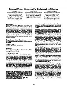
which is induced from available examples. The goal is to produce a classifier that will work well on unseen examples, i.e. it generalises well. Consider the example for a two-dimensional input space in Figure 1; here there are many possible linear classifiers that can separate the data, but there is only one that maximises the margin (maximise the distance between it and the nearest data point of each class). This linear classifier is termed the optimal separating hyperplane. Intuitively, this boundary is expected to generalise well as opposed to the other possible boundaries. The hyperplane (w . x) + b = 0 satisfies the conditions: (w . xi) + b > 0 if yi = 1 (w . xi) + b < 0 if yi = -1
and (7)
By scaling w and b with the same factor, an equivalent decision surface can be formulated as: (w . xi) + b > 1 if yi = 1 (w . xi) + b < 1 if yi = -1
and (8)
which is equivalent to yi [(w . xi) + b ] ≥ 1, i = 1, . . . , l
(9)
The distance d(w,b;x) of a point x from the hyperplane (w,b) is,
Figure 1Optimal separating Hyperplane
d(w,b;x) = | w . x + b | / ||w||
(10)
The optimal hyperplane is then given by maximising the margin, ρ(w, b), subject to the constraints of eqn (9). This margin is calculated as: ρ (w, b) = min d (w, b; x i ) + min d (w, b; x j ) { x i : y i =1}
{ x j : y j = −1}
(11)
Substituting eqn (10) in eqn (11) and further simplification, the margin is given by: ρ(w, b) = 2 / ||w||
(12)
Hence the hyperplane that optimally separate the data is the one that minimises Φ(w) = ||w||2/2
(13)
The solution to the optimisation problem of eqn (10) under the constraints of eqn (9) is given by the saddle point of the Lagrange functional (Minoux [1986]). L(w, b, α) = ||w||2 /2 - ∑ αi{[(w . xi) + b ] yi - 1}
(14)
where αi are the Lagrange multipliers. The Lagrangian has to be minimised with respect to w, b and maximised with respect to αi ≥ 0. In the saddle point the solutions w0, b0 and α0 should satisfy the following conditions: ∂L(w0, b0, α0) / ∂b = 0
⇒
∑ α0i yi = 0
(15)
∂L(w0, b0, α0) /∂w = 0
⇒
w0 = ∑ α0i xi yi
(16)
Only the so-called support vectors can have non-zero coefficients α0i in the expansion of w0 The Kuhn-Tucker theorem states that the necessary and sufficient conditions for the optimal hyperplane are that the separating hyperplane satisfies the conditions: α0i {[( w0 . xi) + b0 ] yi - 1} = 0, i = 1, . . . , l
(17)
as well as being a saddle point. Substituting these results into the lagrangian, and after further simplifications, the following dual form of the function to be optimised is obtained: W(α) = ∑αi – (1/2) ∑∑ αiαj yi yj (xi . xj )
(18)
This function has to be maximised with constraints αi ≥ 0 and ∑ αi yi = 0. Finding solutions for real-world problems will usually require application of quadratic programming optimisation techniques and numerical methods. Once the solution has been found in the form of a vector α0 = (α01, α02, . . . , α0l ),the optimal separating hyperplane is given by w0 = ∑ αi0 xi yi
and
b0 = -(1/2) w0 . [xr + xs]
where xr and xs are any support vector from each class. The classifier can then be constructed as: f(x) = sign(w0 . x + b0) = sign( ∑ yiα0 (xi . x) + b0)
(19)
From the Kuhn-Tuker [1951] condition, only the points xi which satisfy {yi (w0 . x + b0) = 1}, will have non-zero Lagrangian multiplier. These points are termed Support Vectors (SV). If the data is linearly separable all the SV will lie on the margin and hence the number of SV can be very small. Subsequently the hyperplane is determined by a small subset of the training data ; the other points could be removed from the training set and recalculating the hyperplane would produce the same answer. Hence SVM can be used to summarise the information contained in a data set by the SV produced. The above solution only holds for separable data, but has to be slightly modified for nonseparable data by introducing a new set of variables {ξi} that measure the amount of violation of the constraints. Then the margin is maximized, paying a penality proportional to the amount of constraint violation. Formally one solves the following problem: Minimise
Φ(w) = ||w||2/2 + C ( ∑ξi )
Subjected to
yi [(w . xi) + b ] ≥ 1-ξi, and ξi ≥ 0
(20) i = 1, . . . , l
(21)
where C is a parameter chosen a priori and define the cost of constraints violation. The first term in eqn (20) amounts to minimizing the VC-dimention of the learning machine, thereby
minimising the second term in the bound of eqn (5). On the other hand, minimizing the second term in eqn (20) controls the empirical risk, which is the first term in the bound of eqn (5). This approach, therefore, constitutes a practical implementation of Structural Risk Minimisation on the given set of functions. In order to solve this problem, the Lagrangian is constructed as follows: L(w, b, α) = ||w||2 /2 + C ( ∑ξi ) - ∑ αi{[(w . xi) + b ] yi - 1 + ξi} - ∑γi ξi
(22)
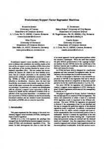
where αi and γi are associated with the constraints in eqn (21) and the values of αi have to be bounded as 0 ≤ αi ≤ C. The solution of this problem is determined by the saddle point of this Lagrangian in a way similar to that described in eqns (14)-(18). In the case where a linear boundary is inappropriate (or when the decision surface is non linear), the SVM can map the input vector x, into a high dimensional feature space z, by choosing a non-linear mapping a priori. Then the SVM constructs an optimal separating hyperplane in this higher dimensional space as shown in Figure 2. Among acceptable mappings are polynomial, radial basis functions and certain sigmoid functions. In this case, the optimisation problems of eqn (18) becomes, W(α) = ∑αi – (1/2) ∑ αiαj yi yj K (xi . xj )
(23)
where K(x,y) is the kernel function performing the non linear mapping into feature space, and the constraints are unchanged. Solving the above equation determines the Lagrange multipliers, and a classifier implementing the optimal separating hyperplane in the feature space is given by, f(x) = sign( ∑ yiα0 K(xi . x) + b0)
(24)
The other case is when the data lies in multiple classes. To get kclass classification, a set of binary classifiers f1, …, fk are constructed, each trained to separate one class from the rest, and combining them by doing the multi-class classification (applying a voting scheme) according to the maximal output before applying the sign function (Scholkopf [1997]), i.e taking: argmaxj = 1, …, k gj(x), where gj(x) = ∑ yiαj K(xi . x) + bj and f(x) = sign(gj(x))
(25)
Figure 1 By mapping the input data nonlinearly into a higher dimensional feature space and constructing a separating hyperplane there, a SV cortresponds to a nonlinear decision surface in input space (adopted from Scholkopf [1997]).
2.2 Support Vector Regression SVMs can also be applied to regression problems by the introduction of an alternative loss function that is modified to include a distance measure (Smola [1996]). Considering the problem of approximating the set of data, ( x1, y1 ), . . . ( xl yl ), x ∈ RN , y ∈ R with a linear function, f (x, α) = (w . x) + b the optimal regression function is given by the minimising the empirical risk, Remp(w, b) = 1/l ∑ | yi – f (xi, α) |ε
(26)
With the most general loss function with ε-insensitive zone described as: | y - f (x, α) |ε = {ε if | y – f (x, α)| ≤ ε; | y – f (x, α)| otherwise }
(27)
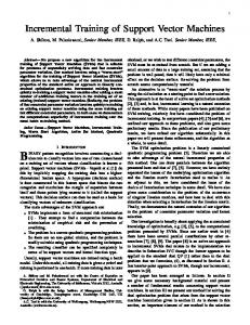
the goal is to find a function f (x, α) that has at most ε deviation from the actual observed targets yi for all the training data, and at the same time, is as flat as possible. This is equivalent to minimising the functional, Φ(w, ξ*, ξ) = ||w|| /2 + C (∑ξi* + ∑ξi )
(28)
where C is a pre-specified value and ξ*, ξ (see Figure 3 ) are slack variables representing upper and lower constraints on the outputs of the system as follows, yi – ((w . xi ) + b) ≤ ε + ξi ((w . xi ) + b) - yi ≤ ε + ξi* ξi* ≥ 0 and ξi ≥ 0
i = 1,2, …,l i = 1,2, …,l i = 1,2, …,l
(29)
Now the Lagrange function is constructed from both the objective function and the corresponding constraints by introducing a dual set of variables as follows: L = ||w||2 /2 + C ∑ (ξi + ξi*) – ∑ αi[ε + ξi - yi + (w . xi) + b ] – ∑ (αi* [ε + ξi* + yi - (w . xi) - b] - ∑ (ηi ξi + ηi* ξi* )
ξ
+ε 0 -ε
(30)
It follows from the saddle point condition that the partial derivatives of L with respect to the primary variables (w, b, ξi, ξi*) have to vanish for optimality. Substitute the results of this derivation in to eqn (30) yields the dual optimisation problem:
Figure 1 Pre-specified accuracy ε and a slack variable ξ in SV regression.
W(α*, α) = -ε∑ (αi* + αi ) + ∑ yi (αi* - αi ) – (1/2) ∑∑ (αi* - αi ) (αj* - αj ) (xi . xj ) that has to be maximised subject to the constraints: ∑ αi* = ∑ αi ; 0 ≤ αi* ≤ C and 0 ≤ αi ≤ C
(31)
for i = 1,2, …,l
Once the coefficients αi* and αi are determined from eqn (31), the desired vectors can now be found as:
w0 = ∑ (αi* - αi ) xi
and therefore f (x) = ∑ (αi* - αi ) (xi . x) + b0
(32)
where b0 = -(1/2) w0 . [xr + xs] Similarly to the non linear support vector classification approach, a non linear mapping kernel can be used to map the data in to a higher dimensional feature space where linear regression is performed. The quadratic form to be maximised can then be rewritten as: W(α*, α) = -ε∑ (αi* + αi ) + ∑ yi (αi* - αi ) – (1/2) ∑ ∑ (αi* - αi ) (αj* - αj )K(xi , xj )
(33)
and the regression function is given by f(x) = w0 . x + b0
(34)
Where w0. x = ∑ (αi0 - αi0*) K(xi , x)
and
b0 = -(1/2) ∑ (αi0 - αi0* )[K(xr , xi)+K(xs , xi)]
(35)
3 Application of SVM 3.1 Features Classification of Digital Remote Sensing Data. Remote sensing image, and information extracted from such images, has nowadays become the major data source for GIS. It is usually done using an aircraft, which commonly provides digital aerial photograph, or using the space sensor on the satellite, which provides satellite images. Classification is one of the important processes of image analysis, which is to automatically categorize all the pixels in the image into the land cover classes such as wood, water, road etc based on pixel spectral and spatial information, which is further used in coupling GIS with hydrological modelling. For the present experiment, the results of previous study (Velickov et al., 2000) on classification of remote sensing data are used. In that study, the digital airborne photographs (total 47) of Athens region were considered. In each source image, there are 4387*2786 pixels and they are stored as Grey-scale TIF format. The prototype of the system developed in the study contains 2 modules, namely: Feature extractor and Self-Organising Feature Map (SOFM) classifier. Extraction of feature from the pattern space is important for classification or pattern recognition. In this way, data can be transformed from the high amount of data in pattern space to smaller amount of data in feature space while the feature can still keep the information in the input pattern (see Figure 4). Data pattern space
Feature extractor
statistical parameters spatial dependence parameners
Features feature space
Class Classifier
SOFM support vector machines
Figure 4. Design of the image recognition system
land cover
Statistic parameters, such as mean and variance and spatial relation parameters (texture) such as Energy, Momentum, Entropy, Correlation, Cluster Shade and Cluster Prominence (which are based on the co-occurrence of its grey level which has values between 0 and 255) are important when doing image analysis. Since each image of the above size is too big to process on a PC, all images were cut into several pieces of the size 1024*1024. From these sub-images, small windows (segments) with the size of 16*16 pixels were chosen randomly, assuming to be characterised by homogeneous texture and statistical parameters. For each chosen window (segment), basic statistic and spatial relation parameters were calculated (see Appendix 1) using the feature extractor. This gives 1024 sample patterns each containing 8 features. Finally, SOFM is used to classify these patterns and then the four discovered classes (namely Agriculture, Meadow, Woods and Scrub and Urban area) were labelled based on the land cover specification from Soil Conservation Service (SCS, 1969??) and statistical and texture parameters extracted from well-known image segments. The main objective of this case study is then to demonstrate the potential of SVM for classification (multi-class in this case) of non-linear systems. In order to achieve that, the 1024 patterns of extracted features (with 8 dimensions) and their corresponding classes obtained from SOFM were used to train SVM. Different types of kernel functions were used during the experiment (presented in the Appendix) and Table 1 summarises results obtained in the training stage. Table 1. Training results of the SVMs Kernel function
Absolute error [%]
simple dot product simple polynomial kernel real polynomial kernel radial basis function full polynomial kernel
24.3 0.195 0.097 0.097 0.097
Total number of support vectors positive SV negative SV 9 8 31 22 32 23 106 133 29 24
Results obtained by training the SVM using simple dot product (which performs well only on linear classification problems) suggested high non-linearity of the feature space. Best results during the training stage were obtained using radial basis and full polynomial kernels. However the number of support vectors found using the radial basis function kernel, which define the shape of the optimal hyperplane, has indicated the costly computational time which is necessary for training of the SVMs. Validation of the SVMs was performed using test remote sensing image with size of 256*256 pixels already labelled with land cover classes (Figure 5a). As the computational uniform unit chosen in this study is window of 16*16 pixels size, the average gray level of each window for the original image is calculated, as shown in Figure 5b. SOFM and SVMs classifiers were used to predict the land cover classes for the test image. The performances for both classifiers are summarised in Table 2 and represented in Figure 5. Table 2. Validation results for SOFT and SVMs classifiers SOFM
Absolute error [%]
3.12
simple dot product
Support Vector Machine simple real radial polynomial polynomial basis kernel kernel function
full polynomial kernel
24.5
0.39
0.00
0.39
0.00
q q q
q
q
q
q
original image (256*256 pixels) gray scale of window average (16*16) class label
reproduced image by the SOFM classifier, gray scale of window average (16*16) predicted class label
reproduced image by the SVM classifier using radial basis and full polynomial kernels, gray scale of window average (16*16) predicted class label
Figure 5. Original test image and reconstructed image by the SOFM and SVM classifiers Validation of the SVM constructed using radial basis function and full polynomial kernels has shown superior performance of the SMV in comparison to SOFM for this particular experiment. 3.2 Prediction of Horizontal Force on Vertical Break Water Vertical breakwaters are upright concrete structures built at sea in order to protect an area from wave attack. They are specifically used in harbour areas with relatively high water depths, where traditional rubble-mound (or rock slope) breakwaters become a rather expensive alternative. The stability analysis of such vertical breakwaters (as in Figure 6) relies on estimation of the total force and overturning moments caused by dynamic wave pressure action (Meer and Franco, [1995]). The total horizontal force of vertical breakwater is the result of the interaction between the wave field, the foreshore and the structure itself (Gent and Boogaard [1998]). The wave field in the offshore region can be described using two standard parameters, namely, the
Figure 6 Vertical breakwater layout and the different parameters involved (adopted from Gent and Boogaard, 1998)
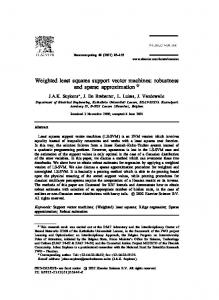
significant wave height in the offshore region (Hs) and the corresponding peak wave period (Tp). The effect of the foreshore is described by the slope of the foreshore (tan θ ) and the water depth in front of the structure (hs). The structure is characterised by the height of the vertical wall below and above the water level (h’ and Rc), the water depth above the rubblemound foundation (d) and the shape of the superstructure (ϕ). The berm-width is also added as additional parameter (Bb). Present day design practice of vertical breakwater mainly depends on physical model tests and empirical formulae. The data used for this study are collected from physical-model tests performed at several laboratories. Based on the published data, the parameter corresponding to the total horizontal force that is exceeded by 99.6% of the wave has been derived (Gent and boogaard, 1998). In total 612 data-patterns have been used from different institutes: 68 by DELFT HYDRAULICS (The Netherlands), 59 by DHI (Denmark), 97 by CEDEX (Spain), 215 HR Wallingford (UK) and 173 by Leightweiss Institute (Germany). One of the best known set of formulae to predict total horizontal forces on vertical structures is the Goda method (Goda [1985]). Recently, Artificial Neural Networks (ANNs) were also applied for the same problem successfully (Gent and Boogaard [1998]). However they followed a slightly modified approach, including explicit physical knowledge, adopted from Froude’s law, in preparing the data for training the network. The input/output patterns were then re-scaled to a form where the Hs0 (equivalent deep-water wave height) become 0.1m (this choice of 0.1 is rather arbitrary). As a result every input output pattern was scaled with different factor λ. In this way a ‘new’ data set still consisting of 612 input/output patterns but the input dimension is reduced from 9 to 8 by removing Hs0. Gent and Boogaard reported that, as a result of this reduction of the input dimension, in addition to the important physical knowledge included in the data, training can be performed with NN of reduced size and complexity. In this study, however, the possibility of using Support Vector Regression (SVR) as yet another data driven modelling approach for prediction of the horizontal force on vertical breakwater has been investigated. The same data set described above is used in order to make comparison with the previous NN modelling results. Five types of kernel functions, namely the simple dot product, simple polynomial, radial basis function, semi-local and linear splines(see Appendix) were used for SVM training. Using the simple dot product kernel amounts approximating with a linear SVM while the rest of the kernels results in non linear SVM. Table 3 shows the RMSE of best performing SVMs for each kernel type with the corresponding numbers of support vectors, while Figure 7a shows the changes in the training and validation RMSE for radial basis function kernel which resulted from different combination of parameters (like C, ε and γ ). It shows that while it is possible to reduce the training error by increasing the capacity of the machine by fine tuning the different parameters, the generalisation ability, however, will eventually deteriorate. The other observation is that an increase in the performance of the machine on the training data usually corresponds with an increase in the number of the corresponding support vectors. This, in its turn, results in a relatively larger computational time and memory requirement. So there should always be a trade off between these factors, which is also true in case of ANN applications. In the present application the SVMs were found to generalisation well by setting the capacity factor C between 10 and 100. Similarly, in most cases, ε values in the range of 0.01 to 0.025 resulted in the best performing SVM. For radial basis function and semi-local kernels, γ values in the range of 3 to 10 were found to be appropriate.
Table 3 General performance of SVMs with different kernel functions Kernel function RMSE Total number of support vectors Training Testing positive SV Negative SV simple dot product 0.311 0.288 143 146 simple polynomial 0.218 0.219 129 138 radial basis function 0.208 0.199 213 222 semi-local 0.174 0.210 142 131 linear splines 0.211 0.191 119 133 ANN(with sigmoid tran. fun.) 0.203 0.186 As one can see from Table 3, the general performance of the SVM (especially with radial basis and linear spline kernels) is quite comparable with that of ANN’s with mean absolute errors (both in training and testing) of less than 10% of the data range. However one can also see that SVM predicted the output quite well in the lower and middle range of the data set while ANN seems to predict the higher range of the output values relatively better. For both cases, large scatter is observed which is to a large extent caused by the quality of the measured data (see Gent and Boogaard []). The over all results of this investigation, however, show that SVMs are still able to provide realistic predictions of forces on vertical structures. SVM w ith Radial Basis Kernel
0.6
2
0.5 1.6
RMSE
Predicted Fh
0.4
0.3
0.2
0.1
1.2
0.8
0.4
0 1
2
3
4
5
6
7
8
9
10
11
12
13
14
15
16
0
17
0
Case No. Training
0.8
1.2
Measured Fh
Testing
SVM w ith Linear Splines Kernel
1.6
Training
2
Testing
ANN w ith Sigmoid Transfer Functions
2
2
1.6
1.6
Predicted Fh
Predicted Fh
0.4
1.2
0.8
0.4
1.2
0.8
0.4
0
0 0
0.4
0.8
1.2
Measured Fh
1.6
Training
2
Testing
0
0.4
0.8
Measured Fh
1.2
1.6
Training
Figure 7 Scattered plot of predicted verses measured output from SVMs and ANN
2
Testing
4. Conclusions and Recommendations In this paper the main principles of SVM are reviewed and it has been shown that they provide a new approach for feature classification and multiple regression problems with clear connections to the underlying statistical learning theory. In both cases SVM training consists of solving a – uniquely solvable – quadratic optimization problem, unlike the ANN training, which requires non-linear optimisation with the possibility of getting stuck in local minima. For digital remote sensing data, SVM classifies the four features distinctively with better performance than SOFM. SVM has also shown a satisfactory performance for prediction of forces on vertical structures due to dynamic waves. In this case the performance of SVM was comparable to ANN trained with sigmoid transfer function. A SVM is largely characterised by the choice of its kernel, as a result it is required to choose the appropriate kernel for each application cases to get satisfactory results. SVMs are attractive approach to data modelling and have started to enjoy increasing adoption in the machine learning and computer vision research communities. This paper shows the potential of SVMs for application in civil engineering problems. However, several things remain: determining the proper parameters C and ε is still sub-optimal and computationally intensive. A second limitation is speed and the maximum size of the training set. These are some of the areas where more researches are needed.
References 1. 2. 3. 4. 5. 6. 7.
8. 9. 10. 11. 12. 13. 14.
Gent, M. R.A. and Boogaard, H. v.d., Neural Network and Numerical Modelling of Forces on Vertical Structures, MAST-PROVERBS report, Delft Hydraulics, 1998. Goda, Y., Random Seas and Design of Maritime Structures. University of Tokyo Press, 1985. Gunn, S., Support Vector Machines for Classification and Regression, ISIS Technical Report, 1998. Kuhn, H. W., and Tucker, A. W., Nonlinear programming, In Proc. 2nd Berkeley Symposium on Mathematical Statistics and Probabilistics, pp. 481-492, Berkeley, 1951. Meer, J.W. v.d and Franco, L., Vertical breakwaters, Delft hydraulics publications No. 487, 1995. Minoux, M., Mathematical Programing: Theory and Algorithms, John Wiley and Sons, 1986. Osuna, E., Freund, R. and Girosi, F., An improved training algorithm for support vector machines, In Proc. of the IEEE Workshop on Neural Networks for Signal Processing VII, pp. 276-285, New York, 1997. Platt, J., Sequential Minimal Optimization: A fast algorithm for training support vector machines, Technical report MSR-TR-98-14, Microsoft Research, 1998. Scholkopf, B., Support Vector Learning, R. Oldenbourg, Munich, 1997. Smola, A., Regression Estimation with Support Vector Learning Machines, Technische Universitat Munchen, 1996. Vapnic, V., Statistical Learning Theory, Wiley, New York, 1998. Vapnik, V., and Chervonenkis, Theory of Pattern Recognition [in Russian], Nauka, Moscow, 1974. Vapnik, V., The Nature of Statistical Learning Theory, Springer, New York, 1995. Velickov S., Solomatine D.P., Xinying Y. and R.K. Price, Application of data mining technologies for remote sensing image analysis, to be published on the Proc. of the 3rd International Conference on Hydroinformatics (2000), Iowa City, USA.
APPENDIX Table 1. Selected Features Descriptor Mean Variance
Formula 1 n ∑ Xi n i =1 n n s2 = ∑ Xi − X n - 1 i =1
X=
(
)
2
Ng Ng
Energy
∑∑ p
Entropy
− ∑∑ pij log p ij (for pij≠0)
j =1 i =1
2 ij
Ng Ng
j =1 i =1
Ng Ng
Momentum
− ∑∑ (Gi − Gj ) 2 p ij j =1 i =1
Ng Ng
Cluster Shade
∑∑ ((Gi − µ )(Gj − µ i
j =1 i =1
j
)) 3 pij
Ng Ng
Cluster prominence Correlation
∑∑ ((Gi − µ )(Gj − µ j =1 i =1
i
j
)) 4 pij
Ng Ng
(Gi − µ i )(Gj − µ j )
j =1 i =1
σ iσ j
∑∑
Where : Gi is the the gray scale with the rank of i P ij is the normalized co-occurrence matrix
pij
Descriptor
Formula Ng
Ng
i =1
j =1
µ i = ∑ Gi ∑ p ij
Ng
Ng
i =1
j =1
σ i = ∑ (Gi − µ i ) 2 ∑ pij