SUPPORT VECTOR MACHINES FOR CLASSIFICATION AND MAPPING OF RESERVOIR DATA
Mikhail Kanevski Stephane Canu Patrick Wong
Aleksey Pozdnukhov Michel Maignan Syed Shibli
IDIAP RR-01-04
January 2001 To be published as a chapter of the Springer book on soft computing for reservoir characterisation
2
Support Vector Machines for Classification and Mapping of Reservoir Data
M. Kanevski 1,3,4, A. Pozdnukhov2 , S. Canu3 , M. Maignan4 , P.M. Wong5 , S.A.R. Shibli 6 1
IDIAP – Dalle Molle Institute of Perceptual Artificial Intelligence, Simplon 4, Case Postale 592, 1920 Martigny, Switzerland,
[email protected] 2 Moscow State University and IBRAE, Moscow, Russia 3 INSA, Rouen, France,
[email protected] 4 University of Lausanne,
[email protected] 5 University of New South Wales, Australia 6 Landmark Graphics Abstract. Support Vector Machines (SVM) is a new machine learning approach based on Statistical Learning Theory (Vapnik-Chervonenkis or VC-theory). VCtheory has a solid mathematical background for the dependencies estimation and predictive learning from finite data sets. SVM is based on the Structural Risk Minimisation principle, aiming to minimise both the empirical risk and the complexity of the model, providing high generalisation abilities. SVM provides non-linear classification SVC (Support Vector Classification) and regression SVR (Support Vector Regression) by mapping the input space into high-dimensional feature space using kernel functions, where the optimal solutions are constructed. The paper presents the review and contemporary developments of the advanced methodology based on Support Vector Machines (SVM) for the analysis and modelling of spatially distributed information. The methodology developed combines the power of SVM with well known geostatistical approaches and tools including exploratory data analysis and exploratory variography. Real case studies (classification and regression) are based on reservoir data with 294 vertically averaged porosity data and 2D seismic velocity and amplitude. A porosity classification and regression maps are generated using SVC/SVR and the results are compared with geostatistical models.
1 Introduction Support Vector Machines (SVM) is a new machine learning approach based on Statistical Learning Theory (Vapnik-Chervonenkis or VC-theory). VC-theory has a solid mathematical background for the dependencies estimation and predictive learning from finite data sets. SVM is based on the Structural Risk Minimisation
3
principle, aiming to minimise both the empirical risk and the complexity of the model, providing high generalisation abilities. It can be applied for regression and probability density function estimation and hence it is suitable for solving many reservoir characterisation problems. SVM provides non-linear classification by mapping the input space into high-dimensional feature space using kernel functions, where the maximal separating margins are constructed. Using different kernels we obtain learning machines analogous to the well-known architectures (e.g., RBF neural networks, multilayer perceptrons). The performance of the SVM can be improved by kernel modification in a data-dependent way. It allows to build very flexible models to solve wide variety of classification and regression tasks. In the present study radial basis function kernel is mainly used. By varying SVM hyper-parameters (parameters that are tuned by the user outside the machine) it was possible to cover wide region of possible solutions – from overfitting to oversmoothing. The paper presents the review and contemporary developments of the advanced methodology based on Support Vector Machines (SVM) for the analysis and modelling of spatially distributed information. The methodology developed for the spatial data combines the power of SVM with well known geostatistical approaches and tools including exploratory data analysis and exploratory variography. We will present results using a reservoir data set with 294 vertically averaged porosity data. A porosity map is generated using SVM and the results are compared with geostatistical models and simulations. The present study develops the ideas of adaptation of Support Vector Machines to spatial data presented in (Kanevski et al 1999, Kanevski and Canu 2000). Tutorials, publications, software, data, list on SVM applications (including references on speach recognition, pattern recognition and image classification, object detection, function approximation and regression, bioinformatics, time series predictions, data mining, etc.) can be found on (www.kernel-machines.org, 2001).
2 Support Vector Machines Classification Let us present short description of SVM application to the classification problems. Detailed theoretical presentation of the SVM can be found in (Burgess 1998 and Vapnik 1998) on which the presentation below is based. Traditional introduction to the SVM classification is the following: 1) binary (2 class) classification of linearly separable problem; 2) binary classification of linearly non-separable problem, 3) non-linear binary problem 4) generalisations to the multi-class classification problems. First results on application of Support Vector Classifiers (binary classification of pollution data, multi-class classification of environmental soil types data) can be found in (Kanevski et al 1999, Kanevski et al 2000a,b). 2 The following problem is considered. A set S of points (xi) is given in R (we are working in a two dimensional xi = [x1, x2] space). Each point xi belongs to
4
either of two classes and is labeled by yi ∈ {-1,+1}. The objective is to establish an equation of a hyper-plane that divides S leaving all the points of the same class on the same side while maximising the minimum distance between either of the two classes and the hyper-plane – maximum margin hyper-plane. Optimal hyper-plane with the largest margins between classes is a solution of the constrained optimisation problem considered below. 2.1 Linearly separable case Let us remind that data set S is linearly separable if there exist W ∈ R , b ∈ R , such that 2
Yi (W T X i + b) ≥ +1, i = 1,...N
(1)
The pair (W,b) defines a hyper-plane of equation
(W T X + b ) = 0 Linearly separable problem: Given the training sample {Xi, Yi} find the optimum values of the weight vector W and bias b such that they satisfy constraints
Yi (W T X i + b) ≥ +1, i = 1,...N
(2)
And the weight vector W minimises the cost function (maximisation of the margins)
F (W ) = W T W / 2
(3)
The cost function is a convex function of W and the constraints are linear in W. This constrained optimization problem can be solved by using Lagrange multipliers. Lagrange function is defined by N
[
]
L(W , b, α ) = W T X / 2 − ∑ α i Yi (W T X i + b) − 1 i =1
where Lagrange multipliers
αi ≥ 0
The solution of the constrained optimisation problem is determined by the saddle point of the Lagrangian function L(W , b, α ) which has to be minimised with respect to W and b and to be maximised with respect to α . Application of optimality condition to the Lagrangian function yields N
W = ∑ α i Yi X i
(4)
i =1
5
N
∑α Y i =1
i i
=0
(5)
Thus, the solution vector W is defined in terms of an expansion that involves the N training data. Because of constrained optimisation problem deals with a convex cost function, it is possible to construct dual optimisation problem. The dual problem has the same optimal value as the primal problem, but with the Lagrange multipliers providing the optimal solution. The dual problem is formulated as follows: maximise the objective function N
N
i =1
i =1
Q(α ) = ∑ α i − (1 / 2)∑ α iα j Yi Y j X iT X j
(6)
Subject to the constraints N
∑α Y i =1
i i
=0
(7)
α i ≥ 0, i = 1,...N
(8)
Note that the dual problem is presented only in terms of the training data. Moreover, the objective function Q(α) to be maximised depends only on the input patterns in the form of a set of dot products {XiTXj}i=1,2,…N . After determining optimal Lagrange multipliers α i 0 , the optimum weight vector is defined by (4) and the bias is calculated as follows
b = 1 − W T X iS , for Y ( s ) = +1 Note that from the Kuhn-Tucker conditions it follows that
[
]
α i Yi (W T X i + b) − 1 = 0
(9)
α i that can be nonzero in this equation are those for which constraints are satisfied with the equality sign. The corresponding points Xi , called Support Vectors, are the points of the set S closest to the optimal separating hyper-plane. Only
In many applications number of support vectors is much less that original data points. The problem of classifying a new data point X is simply solved by computing
F ( X ) = sign(W T X i + b)
(10)
with the optimal weights W and bias b.
6
2.2 SVM classification of non-separable data: Soft margin classifier In case of linearly non-separable set it is not possible to construct a separating hyper-plane without allowing classification error. The margin of separation between classes is said to be soft if training data points violate the condition of linear separability and the primal optimisation problem is changed by using slack variables. Problem is posed as follows: given the training sample {Xi,Yi} find the optimum values of the weight vector W and bias b such that they satisfy constraints
Yi (W T X i + b) ≥ +1 − ξ i , ξ i ≥ 0, ∀i
(11)
The weight vector W and the slack variables ξi minimise the cost function N
F (W ) = W T W / 2 + C ∑ ξ i
(12)
i =1
where C is a user specified parameter (regularisation parameter is proportional to 1/C). The dual optimisation problem is the following: given the training data maximise the objective function (find the Lagrange multipliers) N
N
i =1
i =1
Q(α ) = ∑ α i − (1 / 2)∑ α iα j Yi Y j X iT X j
(13)
Subject to the constraints (7) and
0 ≤ α i ≤ C , i = 1,...N
(14)
Note that neither the slack variables nor their Lagrange multipliers appear in the dual optimisation problem. The parameter C controls the trade-off between complexity of the machine and the number of non-separable points. The parameter C has to be selected by the user. This can be done usually in one of two ways: 1) C is determined experimentally via the standard use of a training and testing data sets, which is a form of re-sampling; 2) It is determined analytically by estimating VC dimension and then by using bounds on the generalisation performance of the machine based on a VC dimension (Vapnik 1998). 2.3 SVM non-linear classification In most practical situations the classification problems are non-linear and the hypothesis of linear separation in the input space is too restrictive. The basic idea of Support Vector Machines is 1) to map the data into a high dimensional feature space (possibly of infinite dimension) via a non-linear
7
mapping and 2) construction of an optimal hyper-plane (application of the linear algorithms described above) for separating features. The first item is in agreement of Cover’s theorem on the separability of patterns which states that input multidimensional space may be transformed into a new feature space where the patterns are linearly separable with high probability, provided: 1) the transformation is non-linear; 2) the dimensionality of the feature space is high enough (Haykin 1999). Cover’s theorem does not discuss the optimality of the separating hyper-plane. By using Vapnik’s optimal separating hyper-plane VC dimension is minimised and generalisation is achieved. Let us remind that in the linear case the procedure requires only the evaluation of dot products. Let ϕ j ( x) denote a set of non-linear transformation from the input
{
}
j =1,... m
space to the feature space; m – is a dimension of the feature space. Non-linear transformation is defined a priori. In the non-linear case the optimisation problem in the dual form is following: given the training data maximise the objective function (find the Lagrange multipliers) N
N
i =1
i =1
Q(α ) = ∑ α i − (1 / 2)∑ α iα j Yi Y j K ( X iT X j )
(15)
Subject to the constraints (7) and (14). The kernel in (15) is m
K ( X , Y ) = ϕ T ( X )ϕ (Y ) = ∑ ϕ j ( X )ϕ j (Y )
(16)
j =1
Thus, we may use inner-product kernel K(X,Y) to construct the optimal hyperplane in the feature space without having to consider the feature space itself in explicit form. The optimal hyper-plane is now defined as N
f ( X ) = ∑α jY j K ( X , X j ) + b
(17)
j =1
Finally, the non-linear decision function is defined by the following relationship:
[
F ( X ) = sign W T K ( X , X j ) + b
]
(18)
The requirement on the kernel K(X, Xj) is to satisfy Mercer’s conditions (Vapnik 1998). Three common types of Support Vector Machines are widely used: Polynomial kernel
K ( X , X j ) = ( X T X i + 1) p
(19)
8
where power p is specified a priori by the user. Mercer’s conditions are always satisfied. Radial basis function RBF kernel is defined by
{
K ( X , X j ) = exp − X − X j
2
/ 2σ 2
}
(20)
Where the kernel bandwidth σ (sigma value) is specified a priori by the user. In general, Mahalanobis distance can be used. Mercer’s conditions are always satisfied. Two-layer perceptron
{
K ( X , X j ) = tanh β 0 X T X j + β 0
}
(21)
Mercer’s conditions are satisfied only for some values of β0 β1. For all three kernels (learning machines), the dimensionality of the feature space is determined by the number of support vectors extracted from the training data by the solution to the constrained optimisation problem. In contrast to RBF neural networks, the number of radial basis functions and their centres are determined automatically by the number of support vectors and their values. In the present study only the results obtained with the RBF kernel are presented. 2.4 Multi-class classification If there is a binary classifier, the multi-class (M class) classification problem can be solved by the different reductions of primary problem to several dichotomies. (Mayoraz and Alpaydin 1998, Weston and Watkins 1998, Vapnik 1998). The most evident method is one-to-rest or one-against-all classification when M binary classification models, one per each class is developed. Thus, M decision functions are derived, one for each class. Final classification label for validated point is assigned by
y
j
= arg max m
∑
λ (i m ) y i K ( x , x i ) + b ( m )
(22)
i
Second possibility is pair-wise classification when M(M-1) binary classification models are developed. Another way is direct generalisation of SVM to M-class problems. The main disadvantage of this method is that the QPproblem size becomes very large. One-to-rest and pair-wise schemes seem to give satisfactory results in the geostatistical applications.
3 Spatial Data Mapping with Support Vector Regression Assume z∈R is a variable to be predicted based on some geographical observations (x,y). Our work aims at estimating a dependence between z and the
9
geographical co-ordinates based on empirical data (samples) Sn=(xi,yi,zi,εi), i = 1,…n, where • xi,yi, - are the geographical co-ordinates of samples • zi - is the observed or measured quantity. It is assumed to be the realisation of a random variable Zi with an unknown probability distribution Px,y(Z). • εi - is the measurement accuracy for the observation zi • n denotes the sample size
3.1 Prediction problem
3.1.1 The ε-insensitive cost function Assuming f is a prediction function (i.e. a function used to predict the value of Z knowing the geographical co-ordinates), we define the cost of choosing this particular function for a given decision process. First, for a given observation (x,y,z) we define the ε-insensitive cost function:
| f ( x, y ) − z | −ε C{( x, y ), z , ε , f } = 0
if | f ( x, y ) − z |> ε (23) otherwise
where ε characterises some acceptable error. Now, for all possible observations we define the global or generalisation error also known as the integrated prediction error IPE:
IPE ( f ) = ∫ E (C (( x, y, ), z , ε , f ))ω ( x, y )dxdy Z
(24)
where ω(x,y) is some external measure, indicating the relative importance of a mistake at point (x,y). In case of non-homogeneous monitoring networks this function can take into account spatial clustering. Usually ω(x,y) = 1, so that all positions are assumed to be equally important. Our approach is a “cost driven” modelling. For the ε-insensitive cost function it is possible to compute the best prediction function (i.e. the one minimising the IPE). For ω(x,y) = 1, this target function is such that:
∫P
x, y z < r ( x , y ) −ε
( Z )dZ =
∫P
x, y z ≥ r ( x , y )+ε
(Z )dZ
(25)
This function equilibrates the tails of the distribution. For ε = 0 solution
r(x,y) is the conditional median function.
10
3.1.2 Non symmetrical cost function The same calculation can be done for asymmetric cost function. For some practical application, it may appear that the errors under a certain level are not as much important as the errors above (over-estimations and under-estimations are not equivalent). In this case the cost function should be the following
a ( f ( x , y ) − z − ε a ) if (f(x, y) - z) > ε a C d (( x , y ), z , ε , f ) = b ( z − f ( x , y ) − ε u ) (f(x, y) - z) < ε u 0 otherwise where a and b are parameters controlling the asymmetry of the cost function. In this case rs(x,y) the target function minimising the IPE is defined from the following relationship:
∫ bP
x, y z < rs ( x , y ) −ε l
( Z )dZ =
∫ aP
x, y z ≥ rs ( x , y ) + ε a
( Z )dZ
It equilibrates the weighted tails. Other robust cost functions are detailed in (Vapnik, 1998, chapter 11).
3.2 Empirical Risk Minimisation and Structural Risk Minimisation
3.2.1 Function Modelling Let us assume this solution is a function that can be decomposed into two different components: a trend plus a remaining random process. A nice way to take into account this prior, is to look for the solution in a functional space that can be decomposed into two orthogonal subspaces, one modelling the trend, while the other one deals with the remaining random process. Assume H is such a Hilbert space. Assume Kj(x,y) is a basis of the trend component and ϕk, k=1,..m is an orthonormal basis of the remaining part (note that m can be infinity) ∧
m
J
k =1
j =1
f ( x , y ) = ∑ wk ϕ k ( x , y ) + ∑ β j K j ( x , y )
(26) 2
The complexity of the solution can be tuned through ||w|| =Σk=1..mwk2 (Vapnik 1998). Thus, a relevant strategy to minimise IPE is to minimise the empirical error together with maintaining ||w||2 small. This can be obtained by minimising the following cost function:
11
1 minimize || w||2 2 subject to | f ( xi , yi ) - Z i | ≤ ε i , for i = 1,...n
(27)
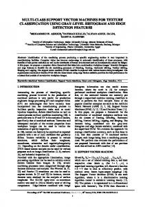
But, unfortunately, some data may lie outside of this epsilon tube due to noise or outliers making these constraints too strong and impossible to fulfil. In this case Vapnik suggests to introduce so called slack variables ξi , ξi* . These variables measure the distance between the observation and the ε tube (see the example in Figure 2.1). The distance between the observation and the ε and ξi , ξi* is illustrated by the following example: imagine you have a great confidence in your measurement process, but the variance of the measured phenomena is large. In this case, ε has to be chosen a priori very small while the slack variables ξi , ξi* are optimised and thus can be large. Remember that inside the epsilon tube ([f(x,y)ε, f(x,y)+ ε ]) cost function is zero.
Figure 1. Support vector regression. Explanation of the ε–tube and slack variables. *
Note that by introducing the couple (ξi , ξi ) the problem has now 2n unknown variables. But these variables are linked since one of the two values is * necessary equals to zero. Either the slack is positive (ξi = 0) or negative (ξi = * 0). Thus, zi ∈ [f(x,y)- ε -ξi, f(x,y)+ ε +ξi ]. Now, we are looking for a solution minimising at the same time its complexity * (measured by ||w||2) and its prediction error (represented by max (ξi , ξi )= ξi + ξi*) . In this case, let us introduce a user specified trade off parameter C between these two contradictory objectives. That leads us to the following problem:
12
n 1 ||ω ||2 + C ∑ (ξ i + ξ *i ) 2 i =1 f ( x i , yi ) − Z i − ε i ≤ ξ i subject to − f ( xi , y i ) + Z i − ε i ≤ ξ *i ξ , ξ * ≥ 0 for i = 1,...n i
minimise
(28)
3.2.2 Dual formulation A classical way to reformulate a constraint based minimisation problem is to look for the saddle point of Lagrangian L:
L(w, ξ , ξ *α ) = n
n n 1 || w ||2 +C ∑ (ξ i + ξ i* ) − ∑α i (Z i − f ( xi , y i ) + ε i +ξ i ) − 2 i =1 i =1
∑α i =1
* i
n
( f ( xi , yi ) − Z i + ε i + ξ i* ) − ∑ (ηiξ i + ηi*ξ i* ) i =1
where α i , α i , η i , η i are Lagrangian multipliers associated with the constraints. They can be roughly interpreted as a measure of the influence of the *
*
constraints in the solution. A solution with α i = α i = 0 can be interpreted as “the corresponding data point has no influence on this solution”. *
At the minimum the derivative of the Lagrangian equals to zero (Kuhn-Tucker conditions). Thus it can be checked that: n
w k = ∑ (α *i − α i )ϕ k ( x i , y i ) for k = 1,...m i =1
η i = C − α i for i = 1,..., n η *i = C − α *i for i = 1,..., n
These variables can be removed from the original formulation of the minimisation problem to get the dual formulation of the problem: m axim ise -
1 2
n
n
∑ ∑ (α i =1 j = 1 n
* i
m − α i ) ∑ ϕ k ( x i , y i ) ϕ k ( x j , y j ) (α *j − α j ) k =1
− ∑ ε i ( α *i + α i ) + i =1 n
subject to
n
∑Z i =1
i
(α *i − α i )
∑ ( α *i − α i ) K j ( x i , y i ) = 0 for K j = 1,... m i=1 0 ≤ α *i , α i ≤ C for i, ... n
13
3.2.3 The nature of the solution To solve the problem without specifying functions ϕk it is necessary to choose ϕk such that: m
∑ϕ k =1
k
(
( x i , yi )ϕ k ( x j , y j ) = G ( x i , yi ), ( x j , y j )
)
(29)
This is the case in reproducing kernel Hilbert space, where G is the reproducing kernel. Functions ϕk are the eigen functions of G. In this case the solution can be formulated in the following form: ∧
n
m
i =1
j =1
f ( x, y ) = ∑ wi G (( x, y ), ( xi , y i )) + ∑ β j K j ( x, y )
(30)
with wi = (α i − α i ) . Note that the function ϕk has disappeared. This solution only depends on the kernel function G. Note also that here at least one of alphas is equalled to zero depending of the observed value zi , above or under the ε-tube. Remark: the solution proposed in equation (30) is the same as the regression spline and kriging estimates (since they are positive definite and reproducing kernels can be interpreted as covariance function (Wahba 1990). The difference between these methods lies in the underlying hypotheses and thus in the way weights in (29) are estimated. In the SVR framework the regularisation is not performed on w but on the representation of the function in some feature space. This is a way to define a regularisation principle that guarantees an explicit bound on the IPE error. From the practical point of view, due to L1 type minimisation, many of the wi can be either zero or C. wi is zero when associated measurement point lies within the ε-tube and thus has no influence on the estimation. This point is useless for the estimation and can be removed without changing the result. wi is equals to C when the associated measurement point is too far from the ε-tube. In this case, the influence of the point is bounded at C. Another way to formulate this remark is to establish the link between SVR and sparse approximation (Girosi 1998). *
3.2.4 Kernel choice As in the case of classification the practical choice for the kernel is the Gaussian kernel:
=
−
−
+
σ
−
(31)
where σ denotes the bandwidth of the kernel. In this case j=1 and the trend function K is a constant.
14
3.2.5 Hyper parameters For practical implementation the hyper parameters of the method have to be tuned. These parameters are the following: • C: although often recommended as very large, geostatistical applications show a great deal of dependence on this parameter. It has to be tuned carefully. • εi : if no additional information is available the easiest way to tune it is to put it small in comparison to standard deviation of data. See below details on influence of the epsilon on training and mapping. In general, it can be related to error measurements and/or small scale variations not resolved by sampling network usually described by nugget effect in variogram. • σ: the bandwidth of kernel. Here again the IPE of the proposed solution is very sensitive to this parameter. More generally, the performance of the solution is sensitive to the distance matrix used in the kernel
4 Case studies. Description of data Let us list the main phases (steps) of the classification/regression studies applied by using SVC/SVR: 1. 2. 3. 4. 5. 6. 7. 8. 9.
Visualisation of data. Monitoring network analysis and description. Understanding of data clustering. Exploratory data analysis. Univariate statistical analysis, outliers detection, data transformation and data pre-processing, trend detection, etc . Exploratory structural analysis (variography). Understanding and modelling of spatial correlations. Splitting data into data sets: Training, Testing, Validation. Training of SVC/SVR with different models. Selection of the optimal SVM hyper-parameters. Pattern completion (categorical data mapping). Regression, spatial predictions of continuous variable. Statistical analysis and variography of the residuals. Understanding and interpretation of the results. Conclusions.
Because of the large differences in magnitude, both porosity and co-ordinate values were re-scaled to between zero and one before any calculations were performed. All mapping and classification results will thus be presented using such re-scaled values; however,, it is understood that the original raw values can be obtained by performing a simple back-transform. Batch statistics and data post plots are presented below. In the present paper two case studies are considered in detail: • Binary classification of porosity data. To pose this problem original continuous data were transformed into “low” and “high” level of porosity. Indicator cut corresponds to the level of 0.5 (about mean value): porosity data higher/less
15
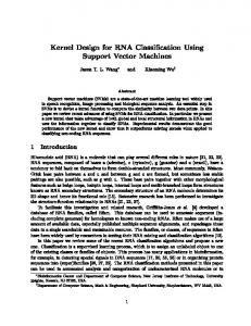
than 0.5 are coded as class +1 and -1. The results of SVC binary classification are compared with indicator kriging. The generalisation of the binary task is a multi class classification problem (Mayoraz and Alpaydin 1998, Weston and Watkins 1998, Kanevski et al. 2000b). Review on geostatistical approach for spatial data classification can be found in (Atkinson and 2000). • Spatial predictions/mapping of porosity data. Support Vector Regression model is developed for the spatial predictions of continuous porosity data. Results of the SVR mapping are compared with ordinary kriging. From the beginning original data were split several times into two data sets: 200 and 94 measurements. The first data set was used to develop SVM models (training data set) and the second one (validation data set) was used to validate the results. Because monitoring network is not clustered, random splitting was used (in case of clustered monitoring networks spatial declustering procedures can be used to have representative testing data set). Another proportions between data sets were used as well. Batch statistics of the entire data set (294 measurements): minimum = 0.0; Q 1/4 = 0.3778; median = 0.515; Q 3/4 = 0.69; max = 1.000e+00; mean = 0.53; variance = 0.048; skewness = 0.12; kurtosis = -0.63. Post plots of training and validation data sets are presented in Figure 2.
Figure 2. Presentation of training data set as area-of-influence polygons. Post plot of testing (“+”) and validation (“O”) data sets.
16
An important phase of spatial data analysis (despite of the methods used) deals with description of spatial continuity using exploratory variography (Chiles and Delfiner 1999). The most widely used measure of spatial continuity for the spatial function Z(x) is a semivariogram
γ ( x , h ) = 12 Var {Z ( x ) − Z ( x + h ) } = E
{(Z ( x ) − Z ( x + h ) ) } = γ ( h ) 2
(32) where h is a separation vector between points in space. In case of intrinsic hypotheses semivariogram (variogram) depends only on separation vector between pairs. The empirical estimate of the semivariogram is given by
γ (h) =
1 2 N (h)
N (h)
∑ ( Z (x ) − Z ( x + h ) ) i =1
i
i
2
(33)
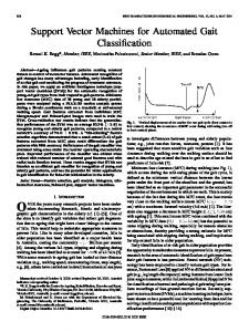
where N(h) is a number of pairs separated by vector h. Variogram rose – semivariogram computed for the different separation vectors for the training data is presented in Figure 3. Geometrical anisotropy is present in the Northeast and Southwest trending directions.
Figure 3. Variogram rose of training data.
In case of second order stationary regionalized random function the relationship between covariance function C(h) and variogram is following: γ(h)=C(0)-C(h).
17
Behaviour of the variogram near the origin at small distances describes the smoothness of the function and characterises the relationship between random and spatially structured parts of information. In the present study the variography is widely used to control the quality of models’ performance.
4.1 Classification of reservoir data In the present paper only the binary classification problem is considered. Original data were transformed into indicators (2 classes) and split into training, testing and validation data set used to develop a model, to tune hyper-parameters (kernel bandwidth and regularisation parameter C) and to validate the model. The splitting was performed several times in different proportions. 4.1.1 Binary classification with Support Vector Machines The particular case of data splitting into training (includes 150 training and 50 testing data points) and validation data (94 data points) sets is presented in Figure 4. The problem is clearly non-linear. Validation data represents different regions classes.
Figure 4. Binary (2 classes) classification problem. “+” – post plot of validation data.
In order to find optimal hyper-parameters comprehensive search was carried out by computing training and testing error surfaces depending on kernel bandwidth and C parameter. The optimal choice is the one with low values of training and testing errors and small values of Support Vectors.
18
The behaviour of the error surfaces is following: • Training error is small and even zero in the region of small kernel bandwidths – overfitting region. All data points are important (overfitting) and are Support Vectors: In this region generalisation is bad and testing error is high. Testing error and number of Support Vectors do not depend on C parameter. For the training error at higher values of C overfitting is achieved at larger values of kernel bandwidths (see Figures 5-7). • In the region of high values of kernel bandwidths (comparable with the scale of the region) there is an oversmoothing. Training error is high and testing error after reaching some minimum at optimal intermediate values of bandwidth is also increasing. In this region the number of Support Vectors is also slowly increasing. • An optimal region is reached at intermediate values of kernel bandwidth and C parameter. In our case the optimal parameters were the following: kernel bandwidths about 0.11 and C=10.
Figure 5. SVM binary classification. Estimate of training error surface.
The classification solution with the optimal hyper-parameters is presented in Figure 8. Validation data are post plot as well. In the following section of the paper the same problem is solved with indictor kriging. Let us remind that the classical output of SVC is deterministic classification, in case of indicator kriging output is a probability map to be above or below the threshold.
19
Figure 6. SVM binary classification. Estimate of testing error surface.
Figure 7. SVM binary classification. Number of Support Vectors surface.
20
Figure 8. SVM optimal classification along with validation data post plot. Filled circles belong to the validation data of white zone class, empty circles belong to validation data of coloured class. Number of Support Vectors (“+”) equals 56.
Thus, in order to make classification, SVC needs only 56 data points (they are Support Vectors). Training error was 4.6%, testing error = 18% and validation error = 11%. Only at the border of decision surface where there is the biggest uncertainty in classification, SVC has some problems with classification of validation data. In fact, it should be taken into account that data can be contaminated by noise and it is not necessary to follow exactly training and validation classes for the particular realisation of the regionalized function. 4.1.2 Binary classification with indicator kriging In order to compare the results of SVM binary classification with geostatistical approach indicator kriging was used. Indicator kriging is a kriging applied to the indicator transformed data:
=
≤
(34)
where zk is a threshold. In terms of probability indicator can be represented as
21
E{ I ( x , z k )} = P{Z ( x ) ≤ z k } = F ( z k )
(35)
Thus, the output of the indicator kriging spatial predictions is interpreted as a probability to be below threshold. It gives a probabilistic interpretation of the binary classification problem. The indicator kriging is a BLUE Best Linear Unbiased Estimator applied to the indicators (Deutsch and Journel 1997). The basic equations of the indicator kriging written in terms of covariance function are following:
F IK ( n
∑λ β =1
k0 β
n
∑λ β =1
k0 β
, z k | { n }) =
n
∑
i=1
λ ki I (
, zk )
(36)
C I ( x β − xα , z k0 ) + µk0 = C I ( x − xα , z k0 ), α = 1,..., n (37) =1
(38)
After exploratory variography based on data, covariance functions/variograms should be modelled. This is performed by fitting the theoretically valid models to the experimental ones. The results of indicator kriging are presented in Figure 9 along with validation data post plot.
Figure 9. Results of indicator kriging (probability to belong to class “O”) along with validation data post plot.
22
The output of indicator kriging is a probabilistic map to be above or below threshold. In our case the interpretation is to belong to one or another class. The solution of indicator kriging is more variable, because of exactitude properties of IK – the solution follows training data points. The same kind of solution can be obtained by SVC by reducing kernel bandwidth moving into overfitting region. Another comments is related to anisotropy. In case of SVC isotropic kernel was used. In case of IK anisotropic variogram model was developed taking into account anisotropic spatial correlations. Next step in the development of SVC deals with the implementation of anisotropic kernels and/or pre-processing of data (e.g., co-ordinates transformations). Finally, other kernels can be applied as well (see Vapnik 1998, where wide choice of kernels is presented).
4.2 Support Vector Regression In the present section the problem of reservoir data mapping – spatial regression – using SVR is considered. 4.2.1 SVR Training In case of SVR there are three hyper-parameters and error cubes should be analysed to find the optimal solution. Comprehensive search in a 3D hyperparameter space was performed. Some 2D errors surfaces with fixed C parameter are presented in Figures 10-12. The same discussion as in the case of classification concerning overfitting and oversmoothing regions is applicable as well. The optimal parameters were chosen taking into account training and testing errors, number of Support Vectors.
Figure 10. Estimate of SVR training error surface. C= 10000
23
Figure 11. SVR testing error surface. C= 10000.
Figure 12. Surface of the number of Support Vectors. C= 10000.
An important phase of the training procedure deals with understanding how much “useful” information was extracted by SVR from data and what is left. In terms of spatial data and geostatistics useful information is spatially structured information. Spatial structures are described basically by variograms. That’s why
24
variographic tools are efficient to understand and to explain the results. In the present study they were used to control the performance of SVR. 4.2.2 SVR Mapping The two particular results of Support Vector Regression mapping are presented in Figures 13 and 14. It should be noted that by varying hyper-parameters it was possible to develop models of very different complexity, covering regions from overfitting to oversmoothing. An interesting oversmoothing case deals with large scale modelling – so called detrending. Non-linearity and flexibility of SVR highly simplifies detrending problem. The quality of detrending can be controlled with geostatistical tools, including variography. Actually, hierarchy of SVR models can be developed to extract anisotropic information from data at different scales and in different regions. One possibility could be mixtures of SVR, another one – local SVR models. An important question, not elaborated in this paper, deals with influence of data pre-processing: linear and non-linear transformations of spatial co-ordinates and data. It seems that in case of anisotropic structures data pre-processing can make them more isotropic and less Support Vectors will be necessary, perhaps leading to better generalisation properties. This problem should be studied with a well defined simulated data sets.
Figure 13. SVR porosity mapping. Kernel bandwidth = 0.1, epsilon parameter = 0.0, all training data are Support Vectors (“O”).
25
Figure 14. SVR porosity mapping. Kernel bandwidth = 0.1, e parameter = 0.08, the number of Support Vectors (“O”) equals 50.
The results on validation data by using SVR(C=10000, kernel bandwidth = 0.1,
ε = 0.08) are presented in Figure 17. Let us remind that only 50 (!) data (Support
Vectors) were used to get almost the same quality of the model as OK. Here we can pose an interesting question about the use of SVR in monitoring network design and redesign. The methodological work in this direction should be related to the developments of corresponding objective functions. Let us remind that in case of OK kriging variance is often used to optimise monitoring network. An analogue of estimation variance can be derived for the SVR based on the training residuals. This approach was applied with General Regression Neural Networks in (Kanevski 1999). 4.2.3 Geostatistical Mapping. Ordinary Kriging Ordinary kriging OK was used as a geostatistical model for the porosity mapping. Ordinary kriging is a BLUE model also based on the analysis and modelling of spatial correlation structures – variography and is described by the following system of equations (n – number of data measurements):
26
n
Z * ( x 0 ) = ∑ wi ( x 0 ) Z ( xi ) i −1
n
∑w γ
j ij
j =1 n
∑w i =1
i
− µ = γ i 0 i=1,…,n
=1
In accordance with geostatistical methodology deep structural analysis – exploratory variography, and modelling were carried out. The main attention during variogram fitting was paid to the directions in which drift is negligible. Geostat Office was used at all stages of geostatistical analysis and modelling. The result of ordinary kriging mapping of porosity data is presented in Figure 15. The same OK model was used to estimate validation data. The results of the validation for SVR models and OK are presented in Figure 16. They are quite good.
Figure 15. Porosity mapping with ordinary kriging.
27
Figure 16. Validation results. SVR and ordinary kriging.
The quality of mapping can be qualitatively described by omnidirectional variograms of the residuals ( see Figure 17.). SVR training residuals demonstrate pure nugget effect – all spatially structured information was extracted by SVR model from data. Nugget effect of the training residuals corresponds to the nugget effect of raw data. The variograms of the validation residuals both of OK model and SVR have pure nugget effect as well. It means good results on validation data.
Figure 17 . Omnidirectional variograms of raw data, SVR training residuals, SVR validation residuals, kriging validation residuals.
28
5 Conclusion The paper presents adaptation of the SVM algorithms – Support Vector Classification and Support Vector Regression to the spatially distributed reservoir data. Two problems were considered in detail: 1) binary classification of spatial categorical data and 2) spatial regression/mapping of porosity data. The basic ideas of SVM training by using errors surfaces was demonstrated. In was shown that near the optimal solution the number of Support Vectors is rather low that is a good indication for low generalisation/validation error. The obtained results are promising that was demonstrated with validation data in both cases. The results were compared with geostatistical approach – indicator kriging in case of classification and ordinary kriging in case of regression. The future developments of the present work deal with the study of kernel types (polynomial, MLP- like, splines, etc.) on the training procedures and final results. An important issue is related the problems of estimation of prediction variance (like kriging variance in geostatistics). This problem can be solved partly by using training residuals. Finally, a generalisation of the SVM to the multivariate case, when quality and quantity of information on different variables differ is of great importance for wider application of SVM approach to environmental data.
6 Acknowledgements The work was supported in part by INTAS grants 97-31726 and 99-00099. Geostat Office software tools were used for the exploratory data analysis, variography and presentation of the results.
7 References Atkinson P. M., and Lewis P. Geostatistical classification for remote sensing: an introduction. Computers and Geosiences, vol. 26 pp. 361-371, 2000. Burgess C. A tutorial on Support Vector Machines for pattern recognition. Data mining and knowledge discovery, 1998. Cherkassky V and F. Mulier. Learning from data. Wiley Interscience, N.Y. 1998, 441 p. Cristianini N. and Shawe-Taylor J. An Introduction to Support Vector Machines and other kernel-based learning methods. Cambridge University Press, 2000 189 pp. Deutsch C.V. and A.G. Journel. GSLIB. Geostatistical Software Library and User’s Guide. Oxford University Press, New York, 1997. Gilardi N. Kanevski, E Mayoraz, M Maignan. Spatial Data Classification with Support Vector Machines. Accepted for Geostat 2000 congress. South Africa, April 2000. Girosi F. An equivalence between sparse approximation and support vector machines. Neural Computation, 10(1), pp. 1455-1480, 1998. Haykin S. Neural Networks. A Comprehensive Foundation. Second Edition. Macmillan College Publishing Company. N.Y., 1999.
29
Kanevski M., N. Gilardi, M. Maignan, E. Mayoraz. Environmental Spatial Data Classification with Support Vector Machines. IDIAP Research Report. IDIAP-RR-9907, 24 p., 1999. (www.idiap.ch) Kanevski M. Spatial Predictions of Soil Contamination Using General Regression Neural Networks. Int. J. on Systems Research and Information Systems, Volume 8, number 4. Special Issue: Spatial Data: Neural nets/Statistics. Guest Editors Dr. Patrick Wong and Dr. Tom Gedeon.Gordon and Breach Science Publishers pp. 241-256. 1999. Kanevski M.. S. Canu. Spatial Data Mapping with Support Vector Regression. IDIAP Reasearch Report; RR-00-09. 2000a. (www.idiap.ch). Kanevski M., A. Pozdnukhov, S. Canu, M. Maignan. Advanced spatial data analysis and modelling with Support Vector Machines. IDIAP Research Report, RR-00-31, 2000b. Kanevski M, V. Demyanov, S. Chernov, E. Savelieva, A. Serov, V. Timonin, M. Maignan. Geostat Office for Environmental and Pollution Spatial Data Analysis. Mathematische Geologie, N3, April 1999, pp. 73-83. Mayoraz E. and E. Alpaydin Support Vector Machine for Multiclass Classification, IDIAPRR 98-06, 1998 (www.idiap.ch). Weston J., Watkins C. Multi-class Support Vector Machines. Technical Report CSD-TR98-04, 9p, 1998. Vapnik V. Statistical Learning Theory. John Wiley & Sons, 1998. Wahba G. Spline Models for Observational Data. No. 59 in regional conference series in applied mathematics, SIAM Philadelphia, Pennsylvania 1990. WWW.kernel-machines.org, 2001.
30