SUPPORTING INFORMATION
Stability Mechanisms of a Thermophilic Laccase Probed by Molecular Dynamics Niels J. Christensen and Kasper P. Kepp* Department of Chemistry, Technical University of Denmark, Kongens Lyngby, Denmark
* Corresponding author E-mail:
[email protected]
S1
RMSD time series for 10 ns NPT equilibrations
Figure S1. RMSD time series for 10 ns NPT equilibration of glycosylated proteins (NAG) in (a) zero ionic strength, (b) 0.3 M NaCl, (c) 0.3 M KF, (d) 1.2 M NaCl, and (e) 1.2 M KF ionic backgrounds.
S2
Figure S2. RMSD time series for 10 ns NPT equilibration of proteins without glycosylation (noNAG) in (a) zero ionic strength, (b) 0.3 M NaCl, (c) 0.3 M KF, (d) 1.2 M NaCl, and, (e) 1.2 M KF ionic backgrounds.
S3
Extended Reference Simulations As discussed in the main text, the 3 ns NVT reference simulation (glycosylated protein, 0.3 M NaCl, 300 K) was extended by 20 ns in four additional simulations with different seeds. Similarly, we extended the following simulations to 20 ns: TvL without glycosylation in 0.3 M NaCl at 300 K, TvL with glycosylation in 0.3 M NaCl at 400 K, and TvL without glycosylation in 0.3 M NaCl at 400 K. The backbone RMSD curves for these simulations are shown in Figure S3a, S3b, and S3c, respectively. The RMSD curve for the non-glycosylated protein at 300 K in 0.3 M NaCl background (Figure S3a) is well-behaved throughout the entire 20 ns simulation. The RMSD curves for the 400 K simulations of the glycosylated protein (Figure S3c) and non-glycosylated protein (Figure S3d) both shows substantial increases after ~3 - 5 ns in agreement with the magnitude of the temperature perturbation.
Figure S3. Backbone RMSD time series for 3ns NVT simulations in 0.3M NaCl background extended to 20 ns. (a) 300 K, without glycosylation. (b) 400 K, with glycosylation. (c) 400 K, without glycosylation. The curves include RMSD for the initial 3 ns simulations.
S4
Time Series for SASA, RMSD, Rgyr, and Backbone HB for 3 ns NVT Simulations NAG_0P0M_300K
Figure S4. Time series of studied properties from 3 ns NVT simulations. a) SASA, b) Backbone RMSD, c) Radius of Gyration, d) Backbone hydrogen bonds.
S5
NAG_0P0M_350K
Figure S5. Time series of studied properties from 3 ns NVT simulations. a) SASA, b) Backbone RMSD, c) Radius of Gyration, d) Backbone hydrogen bonds.
S6
NAG_0P0M_400K
Figure S6. Time series of studied properties from 3 ns NVT simulations. a) SASA, b) Backbone RMSD, c) Radius of Gyration, d) Backbone hydrogen bonds.
S7
noNAG_0P0M_300K
Figure S7. Time series of studied properties from 3 ns NVT simulations. a) SASA, b) Backbone RMSD, c) Radius of Gyration, d) Backbone hydrogen bonds.
S8
noNAG_0P0M_350K
Figure S8 . Time series of studied properties from 3 ns NVT simulations. a) SASA, b) Backbone RMSD, c) Radius of Gyration, d) Backbone hydrogen bonds.
S9
noNAG_0P0M_400K
Figure S9. Time series of studied properties from 3 ns NVT simulations. a) SASA, b) Backbone RMSD, c) Radius of Gyration, d) Backbone hydrogen bonds.
S10
NAG_0P3M_NACL_300K
Figure S10. Time series of studied properties from 3 ns NVT simulations. a) SASA, b) Backbone RMSD, c) Radius of Gyration, d) Backbone hydrogen bonds.
S11
NAG_0P3M_NACL_350K
Figure S11. Time series of studied properties from 3 ns NVT simulations. a) SASA, b) Backbone RMSD, c) Radius of Gyration, d) Backbone hydrogen bonds.
S12
NAG_0P3M_NACL_400K
Figure S12. Time series of studied properties from 3 ns NVT simulations. a) SASA, b) Backbone RMSD, c) Radius of Gyration, d) Backbone hydrogen bonds.
S13
noNAG_0P3M_NACL_300K
Figure S13. Time series of studied properties from 3 ns NVT simulations. a) SASA, b) Backbone RMSD, c) Radius of Gyration, d) Backbone hydrogen bonds.
S14
noNAG_0P3M_NACL_350K
Figure S14. Time series of studied properties from 3 ns NVT simulations. a) SASA, b) Backbone RMSD, c) Radius of Gyration, d) Backbone hydrogen bonds.
S15
noNAG_0P3M_NACL_400K
Figure S15. Time series of studied properties from 3 ns NVT simulations. a) SASA, b) Backbone RMSD, c) Radius of Gyration, d) Backbone hydrogen bonds.
S16
NAG_0P3M_KF_300K
Figure S16. Time series of studied properties from 3 ns NVT simulations. a) SASA, b) Backbone RMSD, c) Radius of Gyration, d) Backbone hydrogen bonds.
S17
NAG_0P3M_KF_350K
Figure S17. Time series of studied properties from 3 ns NVT simulations. a) SASA, b) Backbone RMSD, c) Radius of Gyration, d) Backbone hydrogen bonds.
S18
NAG_0P3M_KF_400K
Figure S18. Time series of studied properties from 3 ns NVT simulations. a) SASA, b) Backbone RMSD, c) Radius of Gyration, d) Backbone hydrogen bonds.
S19
noNAG_0P3M_KF_300K
Figure S19. Time series of studied properties from 3 ns NVT simulations. a) SASA, b) Backbone RMSD, c) Radius of Gyration, d) Backbone hydrogen bonds.
S20
noNAG_0P3M_KF_350K
Figure S20. Time series of studied properties from 3 ns NVT simulations. a) SASA, b) Backbone RMSD, c) Radius of Gyration, d) Backbone hydrogen bonds.
S21
noNAG_0P3M_KF_400K
Figure S21. Time series of studied properties from 3 ns NVT simulations. a) SASA, b) Backbone RMSD, c) Radius of Gyration, d) Backbone hydrogen bonds.
S22
NAG_1P2M_NACL_300K
Figure S22. Time series of studied properties from 3 ns NVT simulations. a) SASA, b) Backbone RMSD, c) Radius of Gyration, d) Backbone hydrogen bonds.
S23
NAG_1P2M_NACL_350K
Figure S23. Time series of studied properties from 3 ns NVT simulations. a) SASA, b) Backbone RMSD, c) Radius of Gyration, d) Backbone hydrogen bonds.
S24
NAG_1P2M_NACL_400K
Figure S24. Time series of studied properties from 3 ns NVT simulations. a) SASA, b) Backbone RMSD, c) Radius of Gyration, d) Backbone hydrogen bonds.
S25
noNAG_1P2M_NACL_300K
Figure S25. Time series of studied properties from 3 ns NVT simulations. a) SASA, b) Backbone RMSD, c) Radius of Gyration, d) Backbone hydrogen bonds.
S26
noNAG_1P2M_NACL_350K
Figure S26. Time series of studied properties from 3 ns NVT simulations. a) SASA, b) Backbone RMSD, c) Radius of Gyration, d) Backbone hydrogen bonds.
S27
noNAG_1P2M_NACL_400K
Figure S27. Time series of studied properties from 3 ns NVT simulations. a) SASA, b) Backbone RMSD, c) Radius of Gyration, d) Backbone hydrogen bonds.
S28
NAG_1P2M_KF_300K
Figure S28. Time series of studied properties from 3 ns NVT simulations. a) SASA, b) Backbone RMSD, c) Radius of Gyration, d) Backbone hydrogen bonds.
S29
NAG_1P2M_KF_350K
Figure S29. Time series of studied properties from 3 ns NVT simulations. a) SASA, b) Backbone RMSD, c) Radius of Gyration, d) Backbone hydrogen bonds.
S30
NAG_1P2M_KF_400K
Figure S30. Time series of studied properties from 3 ns NVT simulations. a) SASA, b) Backbone RMSD, c) Radius of Gyration, d) Backbone hydrogen bonds.
S31
noNAG_1P2M_KF_300K
Figure S31. Time series of studied properties from 3 ns NVT simulations. a) SASA, b) Backbone RMSD, c) Radius of Gyration, d) Backbone hydrogen bonds.
S32
noNAG_1P2M_KF_350K
Figure S32. Time series of studied properties from 3 ns NVT simulations. a) SASA, b) Backbone RMSD, c) Radius of Gyration, d) Backbone hydrogen bonds.
S33
noNAG_1P2M_KF_400K
Figure S33. Time series of studied properties from 3 ns NVT simulations. a) SASA, b) Backbone RMSD, c) Radius of Gyration, d) Backbone hydrogen bonds.
S34
Statistics for Molecular Dynamics Simulations Table S1. Statistics calculated from the last 3 ns NVT MD simulations: Average, Standard Deviation, Minimum and Maximum Values for SASA, Rgyr, and backbone RMSD. 300 K
NAG_0P0M
noNAG_0P0M
NAG_0P3M_NACL
noNAG_0P3M_NACL
NAG_0P3M_KF
noNAG_0P3M_KF
NAG_1P2M_NACL
350 K
400 K
SASA
Rgyr
RMSD
SASA
Rgyr
RMSD
SASA
Rgyr
RMSD
18917
21.93
1.24
18979
21.91
1.23
19149
21.99
1.61
(130)
(0.04)
(0.06)
(198)
(0.04)
(0.07)
(283)
(0.07)
(0.31)
18572 -
21.81 –
1.08 –
18326 -
21.79 –
1.07 –
18442 -
21.80 –
1.12 –
19206
22.01
1.44
19596
22.06
1.47
19882
22.17
2.22
19152
21.95
19271
21.96
1.37
19110
21.93
1.27
(155)
(0.04)
(170)
(0.04)
(0.09)
(236)
(0.05)
(0.09)
18732-
21.87-
18882 -
21.87 –
1.15 –
18474 -
21.81 –
1.07 –
19715
22.07
19728
22.08
1.65
19827
22.06
1.51
19096
21.95
1.25
18825
21.88
1.27
18976
21.91
1.27
(156)
(0.04)
(0.06)
(172)
(0.04)
(0.11)
(196)
(0.05)
(0.09)
18650 -
21.83 –
1.12 –
18354 -
21.76 –
1.05 –
18432 -
21.71 –
1.03 –
19473
22.05
1.43
19260
22.00
1.51
19427
22.02
1.52
19319
21.98
1.07
19149
21.92
1.10
19177
21.98
1.21
(172)
(0.04)
(0.06)
(189)
(0.05)
(0.10)
(210)
(0.05)
(0.10)
18938 –
21.87 –
0.94 –
18490 -
21.78 –
0.91 –
18645 -
21.86 –
0.91 –
19692
22.12
1.23
19545
22.03
1.45
19798
22.12
1.47
19051
21.94
1.00
19088
21.94
1.02
19029
21.92
1.17
(128)
(0.04)
(0.05)
(270)
(0.05)
(0.09)
(183)
(0.05)
(0.13)
18738 -
21.85 –
0.87 –
18496 -
21.76 –
0.82 –
18625 -
21.79 –
0.89 –
19388
22.03
1.13
19916
22.07
1.25
19434
22.06
1.51
19188
21.98
1.20
19122
21.92
1.25
19011
21.96
1.37
(188)
(0.04)
(0.07)
(187)
(0.04)
(0.09)
(260)
(0.06)
(0.13)
18666 -
21.88 –
1.07 –
18630 -
21.82 –
1.10 –
18450 -
21.81 –
1.05 –
19747
22.12
1.40
19658
22.07
1.58
19839
22.14
1.73
19024
21.94
1.07
18948
21.91
1.06
18946
21.88
1.18
(184)
(0.04)
(0.05)
(174)
(0.04)
(0.06)
(221)
(0.06)
(0.08)
18615 -
21.85 –
0.96 –
18438 -
21.80 –
0.91 –
18313 -
21.73 –
0.97 –
1.22 (0.06) 1.10-1.41
S35
noNAG_1P2M_NACL
NAG_1P2M_KF
noNAG_1P2M_KF
19492
22.04
1.24
19551
22.04
1.25
19471
22.02
1.42
18698
21.89
0.99
18679
21.87
1.07
18583
21.86
(132)
(0.04)
(0.04)
(203)
(0.05)
(0.06)
(229)
(0.06)
18347 -
21.80 –
0.86 –
18213 -
21.69 –
0.93 –
18054 -
21.72 –
18975
22.01
1.13
19206
21.99
1.24
19231
22.02
18702
21.86
0.98
18644
21.79
1.09
18622
21.79
1.10
(134)
(0.04)
(0.04)
(148)
(0.04)
(0.06)
(179)
(0.04)
(0.09)
18362 -
21.76 –
0.86 –
18274 –
21.68 –
0.91 –
18148-
21.70 –
0.90 –
19039
21.94
1.09
19036
21.90
1.25
19097
21.09
1.29
19210
21.95
1.05
19090
21.97
1.24
19099
21.95
1.24
(180)
(0.04)
(0.06)
(214)
(0.04)
(0.15)
(228)
(0.05)
(0.12)
18820 -
21.85 –
0.92 –
18581 -
21.88 –
0.96 –
18602 -
21.84 –
0.94 –
19651
22.05
1.25
1959
22.14
1.66
19931
22.09
1.55
1.18 (0.1) 0.93 – 1.49
S36
Radial Distribution Functions for Backbone Amide-H and Halide Anions in 0.3 M Halide Simulations
Figure S34. Top panel: Radial distribution function (RDF) for backbone amide-H and halide anion pairs. Bottom panel: Integrated RDF. Left and right panels correspond to simulations with and without glycosylation, respectively.
S37
Figure S35. Top panel: Radial distribution function (RDF) for backbone amide-H and halide anion pairs. Bottom panel: Integrated RDF. Left and right panels correspond to simulations with and without glycosylation, respectively.
S38
Figure S36. Top panel: Radial distribution function (RDF) for backbone amide-H and halide anion pairs. Bottom panel: Integrated RDF. Left and right panels correspond to simulations with and without glycosylation, respectively.
S39
Figure S37. Top panel: Radial distribution function (RDF) for backbone amide-H and halide anion pairs. Bottom panel: Integrated RDF. Left and right panels correspond to simulations with and without glycosylation, respectively.
S40
Figure S38. Top panel: Radial distribution function (RDF) for backbone amide-H and halide anion pairs. Bottom panel: Integrated RDF. Left and right panels correspond to simulations with and without glycosylation, respectively.
S41
Figure S39. Top panel: Radial distribution function (RDF) for backbone amide-H and halide anion pairs. Bottom panel: Integrated RDF. Left and right panels correspond to simulations with and without glycosylation, respectively.
S42
Persistence of Salt Bridges Table S2. Glycosylated TvLαin NaCl background: Salt bridges found in 3 ns NVT simulations and their persistence (Cons. %) in percentage of 100 frames sampled from 2 last ns of simulations. The simulation average distance (r) in Å between the center of mass of interacting charged groups is also given. Color codes indicate stable salt bridges found in the majority of simulations.
Salt Bridge ASP128-LYS40 ASP138-ARG195 ASP214-ARG260 ASP224-ARG423 ASP42-LYS39 ASP424-ARG243 ASP96-ARG43 GLU288-ARG176
ASP118-ARG22 ASP128-LYS40 ASP138-ARG195 ASP140-ARG199 ASP214-ARG260 ASP224-ARG423 ASP42-LYS39 ASP424-ARG243 ASP96-ARG43 ASP486-LYS482 GLU288-ARG176
ASP118-ARG22 ASP128-LYS40 ASP131-ARG197 ASP214-ARG260 ASP224-ARG423 ASP42-LYS39 ASP424-ARG243 ASP486-LYS482 ASP96-ARG43 GLU288-ARG176 GLU381-ARG440 GLU460-ARG157 ASP138-ARG195
0 M, 300 K 0 M, 350 K Cons. Cons. (%) r (Å) (%) r (Å) 94.0 3.1 96.0 82.0 100.0 3.3 100.0 98.0 3.3 95.0 94.0 2.9 96.0 100.0 3.3 98.0 98.0 3.3 90.0 72.0 3.3 87.0
3.0 3.4 3.3 3.3 2.9 3.3 3.3 3.3
0 M, 400 K Cons. (%) r (Å) 94.0 72.0 96.0 96.0 95.0 90.0
3.0 3.4 3.3 3.4 3.3 3.3
0.3 M NaCl, 300 K 0.3 M NaCl, 350 K 0.3 M NaCl, 400 K Cons. Cons. Cons. (%) r (Å) (%) r (Å) (%) r (Å) 98.0 3.3 72.0 3.3 89.0 3.2 86.0 3.1 94.0 3.1 83.0 3.3 84.0 3.4 81.0 3.4 99.0 3.3 98.0 3.3 97.0 3.3 95.0 3.4 90.0 3.3 89.0 3.4 65.0 3.1 100.0 3.3 99.0 3.3 96.0 3.3 78.0 3.3 81.0 3.3 61.0 2.8 75.0 3.3 1.2 M NaCl, 300 K 1.2 M NaCl, 350 K 1.2 M NaCl, 400 K Cons. Cons. Cons. (%) r (Å) (%) r (Å) (%) r (Å) 77.0 3.3 93.0 3.3 89.0 3.1 89.0 3.0 70.0 3.2 68.0 3.3 100.0 3.3 98.0 3.3 97.0 3.3 98.0 3.4 89.0 3.4 91.0 3.4 98.0 2.9 69.0 2.9 99.0 3.3 100.0 3.3 98.0 3.3 87.0 2.8 51.0 2.8 95.0 3.3 91.0 3.3 86.0 3.3 83.0 3.3 67.0 3.3 62.0 3.3 67.0 3.3 76.0 3.3 76.0 3.4
S43
Table S3. Non-glycosylated TvLαin NaCl background: Salt bridges found in 3 ns NVT simulations and their persistence (Cons. %) in percentage of 100 frames sampled from 2 last ns of simulations. The simulation average distance (r) in Å between the center of mass of interacting charged groups is also given. Color codes indicate stable salt bridges found in the majority of simulations.
Salt Bridge ASP128-LYS40 ASP138-ARG195 ASP140-ARG199 ASP214-ARG260 ASP224-ARG423 ASP42-LYS39 ASP424-ARG243 ASP486-LYS482 ASP96-ARG43 GLU288-ARG176 GLU460-ARG157
ASP128-LYS40 ASP138-ARG195 ASP140-ARG199 ASP214-ARG260 ASP224-ARG423 ASP42-LYS39 ASP424-ARG243 ASP486-LYS482 ASP96-ARG43 GLU288-ARG176
ASP128-LYS40 ASP138-ARG195 ASP140-ARG199 ASP214-ARG260 ASP224-ARG423 ASP42-LYS39 ASP424-ARG243 ASP486-LYS482 ASP96-ARG43 GLU288-ARG176
0 M, 300 K Cons. (%) r (Å) 68.0 3.2 80.0 3.4 88.0 3.4 98.0 3.3 92.0 3.4 97.0 3.0 99.0 3.3 99.0 2.7 89.0 3.3 64.0 3.3 57.0 3.4 0.3 M NaCl, 300 K Cons. (%) r (Å) 85.0 3.1 66.0 100.0 92.0 95.0 99.0
3.4 3.3 3.4 2.9 3.3
0 M, 350 K Cons. (%) r (Å) 76.0 71.0 92.0 99.0 95.0 53.0 99.0 89.0 76.0
0 M, 400 K Cons. (%) r (Å) 3.1 83.0 3.1 3.4 78.0 3.3 3.4 3.3 95.0 3.3 3.4 89.0 3.4 3.0 56.0 2.9 3.3 96.0 3.3 3.3 3.3
88.0 60.0
3.3 3.3
0.3 M NaCl, 350 K 0.3 M NaCl, 400 K Cons. Cons. (%) r (Å) (%) r (Å) 88.0 3.1 66.0 3.1 83.0 99.0 94.0 65.0 96.0
3.4 3.3 3.4 3.0 3.3
53.0 98.0 94.0 84.0
3.4 3.3 3.4 3.3
78.0 2.8 92.0 3.3 87.0 3.3 75.0 3.3 60.0 3.3 1.2 M NaCl, 300 K 1.2 M NaCl, 350 K 1.2 M NaCl, 400 K Cons. Cons. Cons. (%) r (Å) (%) r (Å) (%) r (Å) 93.0 3.1 89.0 3.2 82.0 3.1 97.0
3.3
88.0 100.0 87.0
3.3 3.3 3.4
100.0
3.3
82.0 83.0
3.3 3.3
99.0 93.0
3.3 3.4
99.0 97.0
3.2 3.4
85.0 54.0 85.0 60.0
3.3 2.8 3.3 3.3
93.0
3.3
85.0 52.0
3.3 3.3
S44
Table S4. Glycosylated TvLα in KF background: Salt bridges found in 3 ns NVT simulations and their persistence (Cons. %) in percentage of 100 frames sampled from 2 last ns of simulations. The simulation average distance (r) in Å between the center of mass of interacting charged groups is also given. Color codes indicate stable salt bridges found in the majority of simulations.
Salt Bridge ASP128-LYS130 ASP128-LYS40 ASP138-ARG195 ASP214-ARG260 ASP224-ARG423 ASP424-ARG243 ASP486-LYS482 ASP96-ARG43 GLU288-ARG176 ASP140-ARG199
ASP128-LYS40 ASP214-ARG260 ASP224-ARG423 ASP424-ARG243 ASP96-ARG43 GLU288-ARG176 GLU460-ARG161 ASP486-LYS482 ASP138-ARG195 ASP140-ARG199
0.3 M KF, 300 K Cons. (%) r (Å) 94.0
3.1
99.0 94.0 98.0 88.0 85.0
3.3 3.4 3.3 2.8 3.3
0.3 M KF, 350 K 0.3 M KF, 400 K Cons. Cons. (%) r (Å) (%) r (Å) 97.0 3.0 78.0 3.3 92.0 3.0 87.0 3.4 61.0 3.4 99.0 3.3 99.0 3.3 88.0 3.4 90.0 3.4 99.0 3.3 98.0 3.3 55.0 2.8 94.0 3.3 85.0 3.3 65.0 3.3 68.0 3.3 90.0 3.4
1.2 M KF, 300 K 1.2 M KF, 350 K 1.2 M KF, 400 K Cons. Cons. Cons. (%) r (Å) (%) r (Å) (%) r (Å) 51.4 3.0 99.0 2.9 90.0 3.0 100.0 3.3 98.0 3.3 99.0 3.3 94.4 3.4 99.0 3.3 90.0 3.4 98.6 3.3 98.0 3.3 98.0 3.3 90.3 3.3 94.0 3.3 85.0 3.3 77.8 3.3 74.0 3.3 56.0 3.3 54.2 3.3 66.7 2.8 64.0 3.4 69.0 3.4
S45
Table S5. Non-glycosylated TvLα in KF background: Salt bridges found in 3 ns NVT simulations and their persistence (Cons. %) in percentage of 100 frames sampled from 2 last ns of simulations. The simulation average distance (r) in Å between the center of mass of interacting charged groups is also given. Color codes indicate stable salt bridges found in the majority of simulations.
Salt Bridge ASP128-LYS40 ASP138-ARG195 ASP214-ARG260 ASP224-ARG423 ASP42-LYS39 ASP424-ARG243 ASP96-ARG43 GLU288-ARG176 ASP486-LYS482 ASP140-ARG199
0.3 M KF, 300 K 0.3 M KF, 350 K 0.3 M KF, 400 K Cons. Cons. Cons. (%) r (Å) (%) r (Å) (%) r (Å) 81.0 3.2 83.0 3.1 93.0 3.0 85.0 3.4 82.0 3.4 84.0 3.4 99.0 3.3 95.0 3.3 98.0 3.3 92.0 3.3 94.0 3.3 91.0 3.4 96.0 3.0 81.0 3.0 65.0 2.9 99.0 3.3 99.0 3.3 91.0 3.3 93.0 3.3 93.0 3.3 89.0 3.3 71.0 3.3 71.0 3.3 91.0 2.8 63.0 3.4
ASP128-LYS40 ASP140-ARG199 ASP214-ARG260 ASP224-ARG423 ASP424-ARG243 ASP486-LYS482 ASP96-ARG43 GLU288-ARG176 ASP42-LYS39
1.2 M KF, 300 K 1.2 M KF, 350 K 1.2 M KF, 400 K Cons. Cons. Cons. (%) r (Å) (%) r (Å) (%) r (Å) 92.0 3.0 88.0 3.1 86.0 3.0 90.0 3.4 95.0 3.4 72.0 3.4 100.0 3.3 97.0 3.3 99.0 3.3 88.0 3.4 90.0 3.4 83.0 3.4 100.0 3.3 98.0 3.3 96.0 3.3 90.0 2.8 85.0 2.8 69.0 2.8 98.0 3.3 95.0 3.3 88.0 3.3 78.0 3.3 77.0 3.3 71.0 3.3 95.0 2.9
S46
B-factor Plots for 3 ns NVT MD Simulations NAG_0P0M
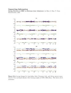
Figure S40. Overlay of reference simulation (red) and current simulation (blue) B-factors for TvLα. The bottom bar indicates secondary structure, with color codes in the upper-left legend. The horizontal three-colored line immediately above the secondary structure bar denotes the three laccase domains (D1: Red, D2: Green, D3: Blue). Above the domain line, short black vertical lines indicate NAG-positions, and red lines denote residues initially 4.5 Å from NAG. Blue and magenta lines indicate residues directly coordinating Cu and immediate structural neighbors of Cu-binding residues, respectively.
S47
noNAG_0P0M
Figure S41. Overlay of reference simulation (red) and current simulation (blue) B-factors for TvLα. The bottom bar indicates secondary structure, with color codes in the upper-left legend. The horizontal three-colored line immediately above the secondary structure bar denotes the three laccase domains (D1: Red, D2: Green, D3: Blue). Above the domain line, short black vertical lines indicate NAG-positions, and red lines denote residues initially 4.5 Å from NAG. Blue and magenta lines indicate residues directly coordinating Cu and immediate structural neighbors of Cu-binding residues, respectively.
S48
NAG_0P3M_NACL
Figure S42. Overlay of reference simulation (red) and current simulation (blue) B-factors for TvLα. The bottom bar indicates secondary structure, with color codes in the upper-left legend. The horizontal three-colored line immediately above the secondary structure bar denotes the three laccase domains (D1: Red, D2: Green, D3: Blue). Above the domain line, short black vertical lines indicate NAG-positions, and red lines denote residues initially 4.5 Å from NAG. Blue and magenta lines indicate residues directly coordinating Cu and immediate structural neighbors of Cu-binding residues, respectively.
S49
noNAG_0P3M_NACL
Figure S43. Overlay of reference simulation (red) and current simulation (blue) B-factors for TvLα. The bottom bar indicates secondary structure, with color codes in the upper-left legend. The horizontal three-colored line immediately above the secondary structure bar denotes the three laccase domains (D1: Red, D2: Green, D3: Blue). Above the domain line, short black vertical lines indicate NAG-positions, and red lines denote residues initially 4.5 Å from NAG. Blue and magenta lines indicate residues directly coordinating Cu and immediate structural neighbors of Cu-binding residues, respectively.
S50
NAG_0P3M_KF
Figure S44. Overlay of reference simulation (red) and current simulation (blue) B-factors for TvLα. The bottom bar indicates secondary structure, with color codes in the upper-left legend. The horizontal three-colored line immediately above the secondary structure bar denotes the three laccase domains (D1: Red, D2: Green, D3: Blue). Above the domain line, short black vertical lines indicate NAG-positions, and red lines denote residues initially 4.5 Å from NAG. Blue and magenta lines indicate residues directly coordinating Cu and immediate structural neighbors of Cu-binding residues, respectively.
S51
noNAG_0P3M_KF
Figure S45. Overlay of reference simulation (red) and current simulation (blue) B-factors for TvLα. The bottom bar indicates secondary structure, with color codes in the upper-left legend. The horizontal three-colored line immediately above the secondary structure bar denotes the three laccase domains (D1: Red, D2: Green, D3: Blue). Above the domain line, short black vertical lines indicate NAG-positions, and red lines denote residues initially 4.5 Å from NAG. Blue and magenta lines indicate residues directly coordinating Cu and immediate structural neighbors of Cu-binding residues, respectively.
S52
NAG_1P2M_NACL
Figure S46. Overlay of reference simulation (red) and current simulation (blue) B-factors for TvLα. The bottom bar indicates secondary structure, with color codes in the upper-left legend. The horizontal three-colored line immediately above the secondary structure bar denotes the three laccase domains (D1: Red, D2: Green, D3: Blue). Above the domain line, short black vertical lines indicate NAG-positions, and red lines denote residues initially 4.5 Å from NAG. Blue and magenta lines indicate residues directly coordinating Cu and immediate structural neighbors of Cu-binding residues, respectively.
S53
noNAG_1P2M_NACL
Figure S47. Overlay of reference simulation (red) and current simulation (blue) B-factors for TvLα. The bottom bar indicates secondary structure, with color codes in the upper-left legend. The horizontal three-colored line immediately above the secondary structure bar denotes the three laccase domains (D1: Red, D2: Green, D3: Blue). Above the domain line, short black vertical lines indicate NAG-positions, and red lines denote residues initially 4.5 Å from NAG. Blue and magenta lines indicate residues directly coordinating Cu and immediate structural neighbors of Cu-binding residues, respectively.
S54
NAG_1P2M_KF
Figure S48. Overlay of reference simulation (red) and current simulation (blue) B-factors for TvLα. The bottom bar indicates secondary structure, with color codes in the upper-left legend. The horizontal three-colored line immediately above the secondary structure bar denotes the three laccase domains (D1: Red, D2: Green, D3: Blue). Above the domain line, short black vertical lines indicate NAG-positions, and red lines denote residues initially 4.5 Å from NAG. Blue and magenta lines indicate residues directly coordinating Cu and immediate structural neighbors of Cu-binding residues, respectively.
S55
noNAG_1P2M_KF
Figure S49. Overlay of reference simulation (red) and current simulation (blue) B-factors for TvLα. The bottom bar indicates secondary structure, with color codes in the upper-left legend. The horizontal three-colored line immediately above the secondary structure bar denotes the three laccase domains (D1: Red, D2: Green, D3: Blue). Above the domain line, short black vertical lines indicate NAG-positions, and red lines denote residues initially 4.5 Å from NAG. Blue and magenta lines indicate residues directly coordinating Cu and immediate structural neighbors of Cu-binding residues, respectively.
S56
Figure S50. Last snapshots from extended (10 ns) NVT simulations at 400 K of TvLα with (left) and without (right) glycosylation in NaCl backgrounds of 0 M (red), 0.3 M (green) and 1.2 M (blue). For reference, the TvLα crystal structure (PDB ID: 1GYC) is included in the upper left corner.
S57
Table S6. Loss of persistent hydrogen bonds for glycosylated TvL in 0.3 M NaCl due to the 300 K to 350 K temperature increase. Hydrogen bonds lost in both the 0.3 M and 1.2 M NaCl background are indicated in bold. acceptor GLY41 GLN45 SER60 ASP77 SER110 HIS111 ASP118 GLY119 ALA134 VAL139 TRP151 LEU158 THR210 ILE274 ASN304 LEU305 SER370 THR383 ASP456 ASP492
donor VAL99 PRO4 GLN499 ASN74 LEU120 SER62 GLN115 TYR116 ASP131 ARG195 ALA168 ALA155 ASN262 PHE270 ILE301 GLU302 PRO367 LEU326 CYS205 CYS488
location β-sheet end first β-sheet, exposed C-terminal, tethering HB α-helical segment, burried β-sheet end, burried β-strand start, end of loop helical segment, burried helical segment, burried loop, exposed β-sheet start, exposed β-sheet turn, exposed Loop, exposed β-sheet start/end, exposed loop, exposed loop/α-helical segment, exposed loop/α-helical segment, exposed turn, exposed β-sheet helix to loop HBond α-helix, C-terminal
S58
Table S7. Loss of persistent hydrogen bonds for glycosylated TvL in 1.2 M NaCl due to the 300 K - 350 K temperature increase. Hydrogen bonds lost in both the 0.3 M and 1.2 M NaCl background are indicated in bold. acceptor VAL27 SER33 ASP42 GLN45 THR51 HIE66 ASP118 ALA134 THR180 ALA241 ASN304 ASP364 LEU365 SER370 THR383 TYR491 ASP492 LEU494
donor VAL30 ARG121 LYS39 PRO4 VAL10 TRP107 THR114 ASP131 SER177 SER202 ILE301 THR361 THR361 PRO367 LEU326 LEU487 CYS488 TYR491
location loop, exposed β-sheet start turn, exposed first β-sheet, exposed β-sheet end, exposed HIE66 involving T3 helical segment, burried loop, exposed loop, exposed turn, burried pointing to T3 site loop/α-helical segment, exposed loop, exposed loop, exposed turn, exposed β-sheet α-helix, C-terminal α-helix, C-terminal C-terminal
S59
Electrostatic Energy Analysis Electrostatics of Persistent Hydrogen Bonds Lost from 300 K to 350 K in both 0.3 M and 1.2 M NaCl Table S8. Simulation averaged electrostatic interaction energy between the residue pairs listed in bold in Table S6 and S7 and persistence of backbone hydrogen bonds for the same residues. The analysis was carried out on the last 2 ns of the 300 K, 350K, and 400 K simulations of glycosylated TvL in 0.3M NaCl. Hydrogen bonds in secondary structure and loop regions are indicated in red and green, respectively. HB
300 K
Location Acceptor Donor
350 K ECoul. Stdev. (kcal/mol) ECoul. -1.98
400 K
α-helix, Cterminal first βsheet β-sheet
Asp492
HB persist. (%) Cys488 65
Gln45
Pro4
92
-5.10
1.16
38
-1.67
1.42
37
-1.60
1.31
Thr383
Leu326 68
-2.04
2.02
41
-1.16
2.25
50
-1.95
3.06
loop
Ala134
Asp131 61
-5.61
1.38
39
-5.81
1.66
43
-5.71
1.77
loop
Asn304
Ile301
69
-3.84
1.03
44
-3.06
1.57
16
-0.84
1.64
turn
Ser370
Pro367 54
-5.11
1.82
50
-5.51
1.71
40
-4.48
1.92
ECoul. Stdev. (kcal/mol) ECoul.
1.55
HB persist. (%) 42
ECoul. (kcal/mol)
Stdev. ECoul.
2.10
HB persist. (%) 25
-0.75
0.29
2.23
Figure S51. Backbone hydrogen bond persistence (a) and electrostatic interaction (b) between the involved residues, averaged across the labile hydrogen bond pairs marked in Table S6 and Table S7. Standard deviations are indicated with error-bars.
S60
Figure S52. Correlation between backbone hydrogen bond persistence (%) and electrostatic energy (kcal/mol) evaluated between the entire residues for (a) residue pairs in structured parts of the protein (red in Table S8), (b) residue pairs in loosely structured parts of the protein (green in Table S8), and (c) residue pairs in both structured and unstructured parts of the protein.
S61
Electrostatics of C-terminal Helix Disruption at Zero Ionic Strength and High Temperature
Figure S53. Electrostatic analysis of the C-terminal unfolding observed for glycosylated TvL in zero ionic background at 400 K (b, d, f), but not at 300 K (a, c, e). The time series show electrostatic interactions between three groups: "water" consisting of all TIP3P molecules, "helix" consisting of the last C-terminal residues 489 - 499, and "protein_nohelix" consisting of the remainder of the protein.
S62
Persistence of Backbone Hydrogen Bonds in Extended Simulations As discussed in the article and above (under Extended Reference Simulations), extended simulations were made in 0.3 M NaCl background for TvL at 300 K with glycosylation (NAG_0P3M_NACL_300K), and without glycosylation K (noNAG_0P3M_NACL_300K). The corresponding simulations at 400 K with and without glycosylation (NAG_0P3M_NACL_400K and noNAG_0P3M_NACL_400K) were also extended. The number of persistent backbone hydrogen bonds (HB) was calculated for the 500 MD snapshots between t = 10 ns and t = 20 ns in each extended molecular dynamics trajectory (Table S9). With reference to the RMSD plot for the simulations (Figure 1 in the article main text and Figure S3 in Supporting Information), it is seen that well-behaved RMSD curves are associated with a larger number of persistent HB. Thus it is only reasonable to compare HB numbers from simulations with equally well-behaved RMSD curves. The extended noNAG_0P3M_NACL_300K simulation yields 164 HB. However, in three out of four simulations with new seeds, the extended NAG_0P3M_NACL_300K simulations have more HB (165 167) than noNAG. This is in agreement with the numbers of persistent HB in the 3 ns NVT simulations for NAG (165) and noNAG (162). The temperature effect is substantial also in the extended simulations: At 400 K, NAG and noNAG have 142 and 144 HB, respectively. In the original 3 ns NVT simulations NAG and noNAG had 148 and 147 HB, respectively. Thus the longer simulation time has decreased the number of persistent hydrogen bonds by ~5 in the high temperature case. In conclusion, the analysis of hydrogen persistence for the longer simulations from new seeds agrees with the major conclusions from the analysis of 3 ns NVT simulations. In particular, the increase in temperature from 300 K to 400 K is associated with a marked reduction of persistence HB, whereas the presence or absence of NAG has a more subtle effect. Table S9. Persistent backbone hydrogen bonds (HB) calculated for the 500 MD snapshots between t = 10 ns and t = 20 ns in extended NVT simulations. extended simulation NAG_0P3M_NACL_300K_Seed1 NAG_0P3M_NACL_300K_Seed2 NAG_0P3M_NACL_300K_Seed3 NAG_0P3M_NACL_300K_Seed4 noNAG_0P3M_NACL_300K NAG_0P3M_NACL_400K noNAG_0P3M_NACL_400K
# persistent HB 155 167 170 165 164 142 144
S63