Nov 20, 2009 - Dept of Software Engineering/B. Thomas Golisano ...... Dr. James Corbett (University of Delaware) provides a framework for policy alternatives.
SUSTAINABLE INTERMODAL FREIGHT TRANSPORTATION: APPLYING THE GEOSPATIAL INTERMODAL FREIGHT TRANSPORT MODEL by Bryan Comer Masters of Science Science, Technology and Public Policy Thesis Submitted in Fulfillment of the Graduation Requirements for the College of Liberal Arts/Public Policy Program at ROCHESTER INSTITUTE OF TECHNOLOGY Rochester, New York November 2009 Submitted by: Bryan Comer Signature
Date
Dr. James W. Winebrake, Thesis Advisor Chair, Dept. STS/Public Policy, College of Liberal Arts Rochester Institute of Technology
Signature
Date
Dr. J. Scott Hawker, Assistant Professor Dept of Software Engineering/B. Thomas Golisano College of Computing and Information Sciences Rochester Institute of Technology
Signature
Date
Dr. Karl Korfmacher, Associate Professor Environmental Science, College of Science Rochester Institute of Technology
Signature
Date
Dr. Franz Foltz, Associate Professor Graduate Coordinator, Dept. STS/Public Policy College of Liberal Arts Rochester Institute of Technology
Signature
Date
Accepted by:
Table of Contents Abstract ................................................................................................................................................. 1 1.
Introduction................................................................................................................................... 1
2.
Literature Review ......................................................................................................................... 7
3.
2.1.
Energy and Environmental Issues Related to Freight Movement ...................................... 7
2.2.
Modal Choices for Freight Transport in the Great Lakes region ....................................... 8
2.3.
Network Optimization Models ............................................................................................. 9
2.4.
My Contribution to the Current State of Knowledge ........................................................ 10
Methodology ............................................................................................................................... 11 3.1. Building an Intermodal Network in a GIS Environment Using a Hub-and-Spoke Approach ......................................................................................................................................... 11 3.2.
Creating the U.S. Intermodal Network .............................................................................. 12
3.3.
Creating the Canadian Network ......................................................................................... 15
3.4.
Creating Spokes ................................................................................................................... 16
3.5.
Reconciling Differences between the U.S. and Canadian Rail and Road Networks ...... 17
3.6.
Using GIFT as a Network Optimization Tool ................................................................... 18
3.7.
The GIFT Emissions Calculator and the Resulting Cost-Factors .................................... 19
3.8.
Data Collection .................................................................................................................... 21
4. Paper 1: Marine Vessels as Substitutes for Heavy-Duty Trucks in Great Lakes Freight Transportation ..................................................................................................................................... 21 4.1.
Abstract ................................................................................................................................ 22
4.2.
My Specific Contributions to Each Section of the Paper ................................................. 22
5. Paper 2: Sustainable Intermodal Freight Transportation: Using Great Lakes Short-Sea Shipping Along an Intermodal Route................................................................................................ 25 5.1.
Abstract ................................................................................................................................ 25
5.2.
My Specific Contributions to Each Section of the Paper ................................................. 26
6. The Need for Public Policy and Policies to Reduce Freight Transport Energy Use and Emissions ............................................................................................................................................ 28 6.1. The IF-TOLD Framework of Policy Levers to Reduce Energy Use and Emissions from Freight Transport ............................................................................................................................ 28 6.2.
Infrastructure Investment .................................................................................................... 29
6.3.
Economic Incentives and Penalties .................................................................................... 34
6.3.1.
Modal Subsidies and Grants ....................................................................................... 34
6.3.2.
Fuel Taxes .................................................................................................................... 35 i
6.3.3.
Carbon Taxes ............................................................................................................... 36
6.3.4.
Cap-and-Trade Programs ............................................................................................ 37
6.4.
Technology Implementation ............................................................................................... 39
6.5.
The Benefits of Intermodalism and Mode-Shifting .......................................................... 40
6.6. Why Public Policies are Necessary to Reduce Freight Transport Energy Use and Emissions ........................................................................................................................................ 41 7.
8.
Limitations of the Model and the Research .............................................................................. 42 7.1.
Speed Limits ........................................................................................................................ 42
7.2.
Delays ................................................................................................................................... 43
7.3.
Energy Use and Emissions .................................................................................................44
7.4.
Impacts of Limitations on Policy Research ....................................................................... 45
Conclusions.................................................................................................................................47
References ........................................................................................................................................... 48 Appendix A ...................................................................................................................................... A-1 Appendix B .......................................................................................................................................B-1
List of Figures Figure 1 - Single mode vs. multi-mode freight transport in the U.S. (ton-mi), 2007....................... 5 Figure 2 - Tons of freight by mode, 2007 ........................................................................................... 5 Figure 3 - Value of U.S. freight by mode, 2007 ................................................................................. 6 Figure 4 - Transportation CO2 emissions, 2006 ................................................................................. 6 Figure 5 - Expected energy use from freight transport by mode through the year 2030. ................ 8 Figure 6 - The Great Lakes portion of the Geospatial Intermodal Freight Transport (GIFT) model showing integration of U.S. and Canadian networks. ...................................................................... 10 Figure 7 - The hub-and-spoke approach to making intermodal network connections in the GIFT model. .................................................................................................................................................. 12 Figure 8 - The anatomy of a shapefile in ArcGIS. ........................................................................... 13 Figure 9 - The U.S. road, rail, and marine shipping networks based on NTAD data, clockwise from top left. ....................................................................................................................................... 14 Figure 10 - The use of Google Earth™ to validate intermodal transport facility locations........... 16 Figure 11 - Reconciling differences between the U.S. and Canadian rail and road networks on the international border............................................................................................................................. 18 Figure 12 - The GIFT Emissions Calculator..................................................................................... 20 Figure 13 - Output from the Emissions Calculator and area to input spoke emission rates and transfer penalties. ................................................................................................................................ 21 Figure 14 - Variables affecting intermodal transfer times. .............................................................. 34
ii
Abstract To study the energy and environmental impacts of emissions associated with freight transportation, the Geospatial Intermodal Freight Transport (GIFT) model was created as a joint research collaborative between the Rochester Institute of Technology (RIT) and the University of Delaware (UD). The GIFT model is a Geographic Information Systems (GIS) based model that links the U.S. and Canadian water, rail, and road transportation networks through intermodal transfer facilities to create an intermodal network. The purpose of my thesis is to apply the GIFT model to examine potential public policies related to intermodal freight transportation in the Great Lakes region of the United States. My thesis will consist of two papers. The first paper will examine the environmental, economic, and time-of-delivery tradeoffs associated with freight transportation in the Great Lakes region and examine opportunities for marine vessels to replace a portion of heavy-duty trucks for containerized freight transport. The second paper will explore the potential benefits of using the Great Lakes as a corridor for short-sea shipping as part of a longer intermodal route. The intent of my thesis is to shed light on the current issues associated with freight transport in the Great Lakes region and present public policy alternatives to address said issues. Ideally, this thesis will better inform policymakers on the impacts and tradeoffs associated with freight transportation. 1. Introduction The key deliverables for my thesis are two publishable papers on Great Lakes freight transportation issues. Given the nature of the research, there are co-authors on each paper. However, as the lead author, I have contributed significantly. In introducing each paper, I will state my specific contributions. The following introduces (1) energy and environmental concerns associated with freight transport, (2) the GIFT model, and (3) the papers. The threat posed by global climate change is mounting. Concentrations of greenhouse gases (GHG) are accumulating in our atmosphere. Though the U.S. has around 5% of the world‟s population, it accounted for approximately 21% of the world‟s GHG emissions in 2003 (U.S. Environmental Protection Agency, 2006a). Most U.S. anthropogenic CO2 emissions come from fossil fuel combustion in the electricity generation and transportation sectors (U.S. Environmental Protection Agency, 2008). These sectors also emit air pollutants that affect human health, such as carbon monoxide (CO), oxides of nitrogen (NO x), sulfur oxides (SOx),
1
particulate matter (PM10), and volatile organic compounds (VOCs). My thesis will focus on emissions from the freight transportation sector. Greenhouse gas emissions from the transportation sector are a major contributor to overall U.S. GHG emissions. In 2003, 27% of the total U.S. GHG emissions were from the transportation sector and GHG emissions growth was greatest in absolute terms in transportation than any other sector between 1990 and 2003 (U.S. Environmental Protection Agency, 2006a). Also, freight transport alone accounted for 9.3% of total U.S. CO2 emissions in 2007 (U.S. Environmental Protection Agency, 2009f). Most U.S. freight is transported unimodally (Figure 1) (Bureau of Transportation Statistics, 2007) and is dominated by trucking in both tons (Figure 2) and value shipped (Figure 3) (Bureau of Transportation Statistics, 2007). Trucks are a carbon-intense mode of freight transport compared to rail and ship on a per container-mile basis and accounted for 19% of total CO2 emissions from the transportation sector in 2007; compare that to 2% for domestic shipping and 1% for rail freight (Figure 4) (Energy Information Administration, 2009a). Freight transportation emissions of CO2 are important because they exacerbate the problem of climate change. Climate change may result in temperature change, precipitation change, seal level rise, and extreme events (Intergovernmental Panel on Climate Change, 2007). These symptoms of climate change may impact ecosystems, water resources, food security, and human health (Intergovernmental Panel on Climate Change, 2007). Emissions of other pollutants from freight transport can also be significant. For example, SO2 emissions can lead to increases in bronchoconstriction (narrowing of the airways), asthma symptoms (Office of Air Quality Planning and Standards, 1994; U.S. Environmental Protection Agency, 2009g), and acid deposition, both dry and wet (acid rain), causing harm to water quality,
2
flora, fauna, and buildings (U.S. Environmental Protection Agency, 2009a). Emissions of PM10 have been linked to human health problems such as increased asthma and other respiratory issues (U.S. Environmental Protection Agency, 2009c). Oxides of nitrogen and VOCs are ground-level ozone precursors. Ozone has been shown to exacerbate respiratory problems in humans and negatively impact plant life (including agricultural crops) (U.S. Environmental Protection Agency, 2009e). Oxides of nitrogen are also a contributor to acid deposition (U.S. Environmental Protection Agency, 2009b). To study the energy, environmental, and economic impacts of associated with freight transportation, the Geospatial Intermodal Freight Transport (GIFT) model was created. The GIFT model is currently under development in a joint research collaborative between the Rochester Institute of Technology (RIT) and the University of Delaware (UD). The GIFT model is a Geographic Information Systems (GIS) based model that connects the U.S. and Canadian water, rail, and road transportation networks through intermodal transfer facilities to create an intermodal network. The GIFT model calculates optimal routing of freight between origin and destination points based on user-defined objectives and is capable of generating intermodal routes. For example, a route may begin on the water network and end on the truck network. The GIFT model not only solves for typical objectives such as least cost and time-ofdelivery, but also for energy and environmental objectives, including least emissions of carbon dioxide (CO2), carbon monoxide (CO), oxides of nitrogen (NOx), sulfur oxides (SO x), particulate matter (PM10), and volatile organic compounds (VOCs). Through the GIFT model, users can evaluate the tradeoffs associated with different goods movement choices, as well as explore how infrastructure development, technology adoption, and economic instruments may affect freight transport decision making.
3
The purpose of my thesis is to apply the GIFT model to two case studies related to public policy in the Great Lakes region of the United States. These cases explore the potential for public policy implementation to reduce the energy and environmental impacts of freight transportation. My thesis will consist of two papers. Though these papers are part of a comprehensive thesis, they could stand alone and may be submitted separately for publication consideration. The first paper will examine the environmental, economic, and time-of-delivery tradeoffs associated with freight transportation in the Great Lakes region and examine opportunities for marine vessels to replace a portion of heavy-duty trucks for containerized freight transport. The second paper will explore the potential benefits of using the Great Lakes as a corridor for short-sea shipping as part of a longer intermodal route. The intent of my thesis is to shed light on how different public policies may affect goods movement in the Great Lakes region. Ideally, this thesis will better inform policymakers on the impacts and tradeoffs associated with freight transportation.
4
Single Mode vs. Multi-Mode Freight Transport in the U.S. (Ton-mi), 2007 Multi-Mode 14%
Single Mode 86% Source: 2007 Commodity Flow Survey Table 1 Figure 1 - Single mode vs. multi-mode freight transport in the U.S. (ton-mi), 2007
Tons of Freight by Mode, 2007 Rail 17%
Water 4%
Air 0%
Truck 79%
Source: 2007 Commodity Flow Survey Table 1 Figure 2 - Tons of freight by mode, 2007
5
Value of U.S. Freight by Mode, 2007 Rail 4%
Air 3%
Water 1%
Truck 92% Source: 2007 Commodity Flow Survey Table 1 Figure 3 - Value of U.S. freight by mode, 2007
Transportation CO2 Emissions, 2006
Air Recreational Boats 10% Shipping, 1%
Shipping, Domestic 1%
Military Use 3%
International 3%
Rail, Freight 2% Freight Trucks 19% Light-Duty Vehicles 58% Bus Transportation 1% Commercial Light Trucks 5/ 2%
Source: AEO 2009, Table 19
Figure 4 - Transportation CO 2 emissions, 2006
6
2. Literature Review The following discusses the current state of knowledge related to intermodal freight transportation generally but with a focus on the Great Lakes region. 2.1. Energy and Environmental Issues Related to Freight Movement Energy use from freight transport nationally and in the Great Lakes region is expected to continue to rise for the foreseeable future, as shown in Figure 5. Much of this growth will occur in the truck and air sectors, which are traditionally the most energy- and carbon-intensive modes of freight transport (U.S. Environmental Protection Agency, 2006b). Because truck transport has a higher energy- and carbon-intensity compared to rail or ship, these trends do not bode well for developing a sustainable freight transportation sector in the U.S. One method of reducing the energy use and emissions from freight transportation is intermodalism and mode-shifting (Winebrake, 2009). For example, shippers could make use of less carbon- and energy-intense modes such as rail and ship rather than truck. Mode-shifting from truck to rail or ship may be beneficial in the Great Lakes region.
7
Projected Energy Use in U.S. Freight Transport, 2006-2030 8000 7000
Trillion BTU
6000
Truck
5000
Rail
4000
Domestic Shipping Air
3000 2000 1000 0 2006 2008 2010 2012 2014 2016 2018 2020 2022 2024 2026 2028 2030
Source: AEO 2009 Table 45
Figure 5 - Expected energy use from freight transport by mode through the year 2030.
2.2. Modal Choices for Freight Transport in the Great Lakes region In the Great Lakes region, decisions on routes and modes of freight transportation are based largely on economic and time-of-delivery considerations. Basing route and transportation mode choices on these metrics alone ignores the inherent tradeoffs associated with freight transport decisions. As an example, an auto parts manufacturer is likely to choose trucking as their mode of freight transport since auto parts are a relatively high-value, time-sensitive good. Shipping by truck may be an optimal decision under a time-of-delivery objective, but may be sub-optimal under sustainability objectives. There are proprietary tools available now that companies use to determine optimal routes based on economics and time-of-delivery criteria. However, these tools neglect to calculate other “costs” associated with route choices, namely, energy and environmental costs. One way to address these growing environmental impacts is through careful consideration of routes along an intermodal freight system (Owens & Lewis, 2002; Winebrake, et al., 2008a). Route selection 8
based on energy and environmental criteria, as opposed to the traditional criteria of cost and time-of-delivery, could help identify environmentally-sustainable ways to move freight throughout the U.S. and abroad (Winebrake, et al., 2008a). The GIFT model is useful in identifying opportunities for intermodal freight in the Great Lakes region. 2.3. Network Optimization Models Network optimization models are used in freight transport logistics (Crainic, 2002). These models are used to find the optimal (least-cost) routes. Costs can include economic, timeof-delivery, emissions, and other factors. As discussed by Winebrake, et al. (2008a), some network optimization models make use of shortest-path algorithms, such as the Dijkstra algorithm (Zhan, 1997). The Dijkstra algorithm is the basis for the Network Analyst extension of Environmental Systems Research Institute‟s (ESRI) ArcGIS 9.3. The GIFT model makes use of Network Analyst to perform its optimal route solving. The GIFT model is not the first network optimization model to be applied to intermodal freight transportation in the U.S., other researchers including Lou and Grigalunas (2002), and Southworth and Peterson (2000) have done so (Winebrake, et al., 2008a). There are some researchers who have introduced intermodal network optimization models in GIS. For example, Winebrake et al. (2008a) note that Boile (2000) applied a GIS based system (TransCAD) with a linear programming approach (GAMS) to conduct shortestpath analysis of intermodal freight movement. They also note that Standifer and Walton (2000) integrated highway, rail, and marine networks in an intermodal GIS environment to study freight transport, as did others (Southworth & Peterson, 2000). The GIFT model connects highway, rail, and shipping networks through ports, railyards, and other transfer facilities to create an intermodal freight transportation network. This 9
intermodal network, connecting both U.S. and Canadian systems, is shown in Figure 6. The GIFT model is developed in ArcGIS 9.3 and uses the ArcGIS Network Analyst tool to conduct its network optimization calculations. What sets the GIFT model apart from other GIS based intermodal networks is the inclusion of economic, time, energy, and environmental attributes, which allows for the analysis of optimal freight routing across a host of objective functions. Tradeoffs associated with different goods movement choices can be explored. We can also model how infrastructure development, technology adoption, and economic instruments may affect freight transport decision making.
Figure 6 - The Great Lakes portion of the Geospatial Intermodal Freight Transport (GIFT) model showing integration of U.S. and Canadian networks.
Source: (Winebrake, et al., 2008b). Created by the author.
2.4. My Contribution to the Current State of Knowledge My thesis builds on the current state of knowledge on intermodal freight transportation and GIS based network optimization tools. Through the two papers, I examine how the Great Lakes can be used to reduce the economic and environmental impacts of freight transportation in 10
the region and suggest public policies that might encourage such use. Specifically, I examine the environmental, economic, and time-of-delivery tradeoffs associated with freight transportation in the Great Lakes region and examine opportunities for intermodal freight transportation, infrastructure development, technology implementation, and economic incentives. 3. Methodology This chapter borrows heavily from previous papers and reports published by the GIFT team (Falzarano, 2008; Falzarano, et al., 2007; Winebrake, et al., 2008a; Winebrake, et al., 2008b) and is included to give the reader a fuller understanding of the GIFT model. Key contributions to this chapter have been made by Dr. J. Scott Hawker (RIT), Dr. Karl Korfmacher (RIT), and Mr. Chris Prokop (RIT). 3.1. Building an Intermodal Network in a GIS Environment Using a Hub-and-Spoke Approach The GIFT model uses a hub-and-spoke approach in order to form a connection between the three modal networks, as shown in Figure 7. Before we proceed to an explanation of how the hub-and-spoke method works, it is important to define the terms “segments” and “spokes.” Network segments refer to actual corridors for freight traffic. For example, a segment would include a portion of an interstate, railroad, or water shipping lane. Network spokes are the artificial connections that we have created in order to connect the three modal networks. Though we have created these connections, they represent real world structures such as rail transfer lines and highway onramps. Spokes connect the road, rail, and water networks through the various U.S. and Canadian intermodal transfer facilities. The transfer facilities are the “hubs” of the huband-spoke approach. This connection is crucial since it allows freight shipments to transfer from one mode to another via actual transfer facilities. Each intermodal transfer facility only includes 11
spokes for those modes it supports. The hub-and spoke approach connects modes directly through facilities using a Pythonbased ArcGIS script we developed that builds an artificial link between appropriate modal networks and the transfer facility. These spokes are “artificial” because they may not follow a physical connection (such as a road) but instead are used as proxy for transfer paths. We can also apply transfer penalties along each of these spokes to represent costs, energy use, time delays, and emissions associated with intermodal transfers. These penalties are integrated into the overall optimization calculations so that they are incorporated in route determination.
Figure 7 - The hub-and-spoke approach to making intermodal network connections in the GIFT model.
Source: (Winebrake, et al., 2008b). Created by Mr. Chris Prokop.
3.2. Creating the U.S. Intermodal Network The GIFT model was originally created with ESRI‟s ArcGIS 9.2 software but was then transferred to ArcGIS 9.3. As shown in Figure 8, shapefiles are vector-based files that serve as the “grid work” for the actual map. These data had to be obtained from various sources since each country (U.S. and Canada) maintains their own data, and GIFT represents transportation networks over geo-political boundaries.
12
The U.S. network was created using shapefiles for road, rail, and marine shipping routes taken from the National Transportation Atlas Database (NTAD), published by the Bureau of Transportation Statistics. The National Transportation Atlas Database is a set of digitized maps of the major transportation networks in the U.S. (road, rail, and water), which are displayed in Figure 9. The U.S. road, rail, and marine shipping networks were sourced from NTAD‟s 2006 spatial data collection and added to create a U.S. transportation network in ArcGIS. After using the 2006 data in our model, NTAD released the 2007 and 2008 versions of their spatial map collection. Our model (created with the 2006 data) was then checked against the NTAD 2007 and 2008 databases. We found that virtually no changes were made between the 2006, 2007, and 2008 data that would affect our model, so we continued to build our network with the NTAD data from 2006. A new database was released by NTAD in 2009 but the GIFT team has not yet checked to see if significant changes have occurred from the 2006 database.
Figure 8 - The anatomy of a shapefile in ArcGIS.
Source: (Winebrake, et al., 2008b). Created by Mr. Chris Prokop.
13
Figure 9 - The U.S. road, rail, and marine shipping networks based on NTAD data, clockwise from top left.
Source: (Winebrake, et al., 2008b). Created by Mr. Chris Prokop.
The National Transportation Atlas Database also includes a list of intermodal transfer facilities, including ports. This list was not, by itself, sufficient as a database of intermodal transfer facilities in the U.S. We modified this list by removing many facilities that obviously do not handle freight (civilian boat ramps are considered intermodal transfer facilities by NTAD) and added some major commercial ports from data provided by the United States Army Corps of Engineers (USACE). The USACE data for facility locations were transformed into point shapefiles using the provided latitude and longitude coordinates, and then introduced into ArcGIS where they were transposed over the NTAD data. We were then able to inspect our maps to see where additional facilities were found with the USACE data. These additional multi-modal facilities, that were absent in the NTAD data, were added to our model. Improving the database of transfer facilities will be an ongoing task as the GIFT model is refined. 14
3.3. Creating the Canadian Network The Canadian map data for road, rail, and water networks came from Transport Canada. Unfortunately, we were unable to source pre-made shapefiles that place multimodal facility locations within Canadian boundaries; so, this piece of the network needed to be manually entered. The data for Canadian port facilities were obtained from online sources that cater to this type of information. Shipping port data for Canada were obtained from Transport Canada and www.worldportsource.com. Multi-modal rail facility data for Canada were obtained from Canadian National (www.cn.ca) and Canadian Pacific (www.cpr.ca). Accurate placement of a facility in a separate shapefile was a manual process involving taking the latitude and longitude coordinates for a particular facility, and then visually inspecting to see that such a facility exists within Google Earth™ (see Figure 10). This methodology worked 100% of the time as each port and rail facility in the Canadian network was visually identifiable within Google Earth™. Occasionally, however, coordinates for a port would mark a spot in the middle of a metropolitan area (usually corresponding to a mailing address), while the actual port could be visually identified in close proximity to this point (and matched by name in Google Earth™). In these instances, coordinates were obtained for a port‟s true location by creating a marker in Google Earth™ over the identifiable port, recording the latitude and longitude, and then transposing those coordinates in ArcGIS.
15
Figure 10 - The use of Google Earth™ to validate intermodal transport facility locations.
Source: (Winebrake, et al., 2008b). Created by Mr. Chris Prokop.
3.4. Creating Spokes Since shapefiles for each transportation network (i.e. rail, truck, and water) are layered and separate from one another, connective links needed to be established to allow the flow of freight from one mode of transportation to another through a rail, truck, or port facility. As discussed above, these features, called “spokes,” are an important piece for completing the network model as they not only offer connectivity between modes of transportation and hubs (facilities), but also hold attribute information for emissions, operation costs, and travel delays that are instrumental in performing complete route analysis. For instance, we can represent the
16
amount of CO2 that is emitted when unloading a container from a ship in a spoke connecting a water route to a facility and then represent the amount of CO2 emitted by loading that container onto a rail car for further transport. With over 3,000 multimodal transfer facilities between the U.S. and Canada, we developed a macro tool to generate spokes between facilities and transport segments automatically. The macro generates connections by taking selected points which represent transfer facilities and creates a link between that hub and the closest endpoint of a line segment representing a road, railway, or marine shipping segment. 3.5. Reconciling Differences between the U.S. and Canadian Rail and Road Networks Finally, rail and road lines between the U.S. and Canada required links where border crossings exist since transportation networks in different spatial localities do not automatically connect. Therefore further connections between road and rail lines were required to model traffic flows over borders. This was performed manually in ArcGIS since there are only a handful of border crossings between these two countries. We used online sources to verify where border crossings do in fact exist and then created the links necessary to connect U.S. and Canadian transportation lines. Figure 11 depicts the process of reconciling differences between the U.S. and Canadian rail and road networks on the international border.
17
Figure 11 - Reconciling differences between the U.S. and Canadian rail and road networks on the international border.
Source: (Winebrake, et al., 2008b). Created by Mr. Chris Prokop.
3.6. Using GIFT as a Network Optimization Tool Our last step in developing GIFT was to integrate the thirteen separate layers of spatial data representing our network between the U.S. and Canada into one seamless network. We used the Network Analyst tool in ArcGIS to do this. With this holistic, intermodal, international network, we are able to model intermodal freight flows from various origin and destination points. At its core, GIFT uses the principles of network optimization and shortest-path algorithms similar to those underlying online mapping systems like Google Maps™ and MapQuest™. A transport system is approximated as a series of points or “nodes” which can be origin, destination, or transit points in the network. Linking the nodes are segments, each with a 18
“weight” that quantifies the cost or distance between two nodes. When two points are selected (origin and destination), the computer calculates the shortest path between the two points by testing a variety of potential routes and selecting the one with the least “weight.” Several methods of shortest path determination have been described in literature, but we use the one described by Dijkstra, which has been repeatedly validated and is the foundation for the Network Analyst tool of ArcGIS (Environmental Systems Research Institute, 1992). The unique feature of the GIFT model is the combination of multiple modes of freight transport into a single network as well as the inclusion of energy and environmental factors as “weights” in the network. The GIFT model solves for the optimal freight transport route by taking into consideration costs along network segments and spokes. The GIFT model is able to solve for optimal routes based on a number of different criteria such as least cost, time, emissions (CO2, NOx, SOx, PM10, CO, and VOCs), and energy through the use of user-defined cost-factors (parameters). 3.7. The GIFT Emissions Calculator and the Resulting Cost-Factors The GIFT team created an Emissions Calculator, shown in Figure 12, allowing the user to input information such as horsepower, fuel economy, cargo capacity, etc. for each mode (truck, rail, and ship). The user can then save their input information as “predefined” trucks, locomotives, and marine vessels to be called up later. The values inputted to the Emissions Calculator are used to calculate “cost-factors.” An example of a cost-factor is the amount of CO2 emitted by a truck carrying a twenty-foot equivalent unit (TEU) container of freight for one mile (grams of CO2 per TEU-mile). Each cost-factor can be modified based on known information about each mode (truck, rail, or ship). Figure 13 shows the output from the Emissions Calculator and shows where the user can input spoke emission rates and transfer penalties. Note that for 19
each mode (truck, rail, and ship) and each intermodal transfer spoke (truck spoke, rail spoke, and ship spoke), values can be added and edited by the user. The user can also input information on truck speed, rail speed, ship speed, and transfer times between modes. These cost-factors are then combined with custom evaluators written as C# program modules that combine the cost data with network data (segment length, speed, etc.) and then called by the ArcGIS Network Analyst as it solves for the optimal route based on the user-defined optimization objective. Data can be retrieved on the accumulated cost, energy, and emissions for the route as well. These data are dependent on the inputs chosen by the user. Because the user can modify the cost factors and inputs, they can adjust them to reflect their own specific operating scenarios, based on current observed data or predicted data resulting from operational changes such as emissions control technologies or adjusted operating costs reflecting carbon tax and trading policies.
Figure 12 - The GIFT Emissions Calculator
20
Figure 13 - Output from the Emissions Calculator and area to input spoke emission rates and transfer penalties.
3.8. Data Collection I have relied on data that currently exists in the GIFT model and have modified those data according to the case I am modeling. My data sources and assumptions are clearly defined in each paper in order to be as transparent as possible. 4. Paper 1: Marine Vessels as Substitutes for Heavy-Duty Trucks in Great Lakes Freight Transportation This chapter will discuss my specific contributions as lead author to Paper 1. I will first include the Abstract of the paper and then go on to detail work I performed for each section. In general, editing for language and correctness was performed by me, Dr. James Winebrake (RIT), Dr. J. Scott Hawker (RIT), Dr. Karl Korfmacher (RIT), Dr. James Corbett (University of Delaware), Dr. Earl Lee (University of Delaware), and Mr. Chris Prokop (RIT). Paper 1 can be found in its entirety in Appendix A.
21
4.1. Abstract This paper applies a geospatial network optimization model to explore environmental, economic, and time-of-delivery tradeoffs associated with the application of marine vessels as substitutes for heavy-duty trucks operating in the Great Lakes region. The geospatial model integrates U.S. and Canadian highway, rail, and waterway networks to create an intermodal network and characterizes this network using temporal, economic, and environmental attributes (including emissions of carbon dioxide, particulate matter, carbon monoxide, sulfur oxides, volatile organic compounds, and nitrogen oxides). A case study evaluates tradeoffs associated with containerized traffic flow in the Great Lakes region, demonstrating how modal choice affects the environmental performance of goods movement. These results suggest opportunities to improve the environmental performance of freight transport through infrastructure development, technology implementation, and economic incentives. 4.2. My Specific Contributions to Each Section of the Paper For the introduction of the paper, I researched previously published works by the GIFT team (Falzarano, 2008; Falzarano, et al., 2007; Winebrake, et al., 2008a; Winebrake, et al., 2008b) that discussed the energy use and emissions from freight transportation and included those observations in the paper. I also researched (1) definitions of the GIFT model‟s capabilities, (2) the methodology used to construct the model, and (3) model improvements, and included this information in the introduction. I sought input from other members of the GIFT team in describing the model in an accurate way. For the background of the paper, I illustrated the energy and environmental impacts of freight transport. I collected data from the Bureau of Economic Analysis, Bureau of Transportation Statistics, and the Energy Information Administration to show a trend of historic and projected growth in vehicle miles traveled (VMT) for freight trucking and ton-miles for rail 22
and domestic marine freight transport. As freight transport activities increase, GHG emissions will also increase. To reduce GHG emissions, particularly CO 2 emissions, in the Great Lakes region, I suggested a shift to less carbon-intense modes of freight transport, such as marine vessels. Some additional research, performed by Dr. James Corbett of the University of Delaware, regarding modal shifts to achieve energy and emissions reduction targets in freight transport was also included in this section. In discussing freight transportation in the Great Lakes region, I reviewed and cited reports and studies conducted by Transportation Economics and Management Systems (TEMS) Inc., RAND, the St. Lawrence Seaway Management Corporation, the St. Lawrence Seaway Development Corporation, and the Great Lakes Maritime Taskforce. I highlighted cargo flows in terms of volume and modal selection (truck, rail, or ship) in the Great Lakes region. I noted that most containerized freight in the region is carried by land-based modes including truck (primarily) and rail. However, I stated that there appears to be interest and room for growth for on-water, containerized freight transport in the Great Lakes region. The modeling approach section of Paper 1 was informed by my discussions with GIFT team members throughout my graduate research. In this section, I discussed what I learned about our approach to constructing the GIFT model. Specifically, I stated that GIFT operates on an ArcGIS 9.3 software platform and uses ArcGIS‟s Network Analyst extension to apply a shortest path algorithm to solve for optimal intermodal freight routes in the U.S. and Canada. The GIFT model is an intermodal network (combining the U.S. and Canadian road, rail, and waterway networks) and can solve for user-defined objective functions. A unique feature of GIFT is that it can solve for the least time, operating cost, energy, and emissions route. Using energy and environmental objective functions, tradeoffs between time and cost savings and
23
emissions reductions can be analyzed. Our modeling approach has been discussed in other published works; however, I authored this section of Paper 1 with input from other GIFT team members, especially when discussing the creation of an intermodal network connected through nodes at intermodal transfer facilities. Dr. J. Scott Hawker, Dr. Karl Korfmacher, and Mr. Chris Prokop were particularly helpful in developing my understanding of the GIFT modeling approach. I authored the Great Lakes case study section of this paper and it was edited by Dr. James Winebrake, Dr. James Corbett, and Dr. Earl Lee. This section discussed the assumptions made for each mode of freight transport that we modeled (truck, rail, and two different marine vessels), how emissions factors were calculated for segments and intermodal transfers, and our assumptions for operating costs and intermodal transfer costs. I researched attributes for each mode including their cargo capacity, horsepower, fuel economy, etc., and consulted other team members to decide on appropriate assumptions for engine efficiency and load factors. Assumptions for transfer emissions were taken from previous research conducted by Mr. Colin Murphy, a recent graduate of RIT and former GIFT team member. The results section of the paper showcased my work in running the GIFT model under various objective functions. I performed a case study examining a route from Montreal, QC to Cleveland, OH. I compared the CO2 emissions, time-of-delivery, and operating cost associated with different modal choices for freight transport (truck, rail, or ship). I conducted this case study myself and generated maps, tables, and graphs to help illustrate the results. The interpretation of the results is my own but some language has been edited by Dr. James Winebrake.
24
The conclusion of the paper is my own. I concluded that trucks are often the fastest mode of freight transportation but emit the greatest amount of CO2. Ships are often the cheapest way to move containers but have a relatively longer time-of-delivery, and some ships offer the lowest CO2 alternative at less cost than trucking. I also discussed that a shift to marine based freight transport in the Great Lakes would require incentives stemming from public policies. These policies might include a carbon tax, port and lock infrastructure improvement and development, and modal subsidies and grants. My conclusion was edited by Dr. James Winebrake and Dr. James Corbett. 5. Paper 2: Sustainable Intermodal Freight Transportation: Using Great Lakes Short-Sea Shipping Along an Intermodal Route This chapter will discuss my specific contributions as lead author on Paper 2. I will first include the Abstract of the paper and then go on to detail work I performed for each section. In general, editing for language and correctness was performed by me, Dr. James Winebrake (RIT), Dr. J. Scott Hawker (RIT), Dr. Karl Korfmacher (RIT), Dr. James Corbett (University of Delaware), and Mr. Chris Prokop (RIT). Paper 2 can be found in its entirety in Appendix B. 5.1. Abstract This paper applies a geospatial network optimization model to explore environmental, economic, and time-of-delivery tradeoffs associated with intermodal freight transportation. The geospatial model integrates U.S. and Canadian highway, rail, and waterway networks to build an intermodal network and characterizes this network using temporal, economic, and environmental attributes (including emissions of carbon dioxide, particulate matter, carbon monoxide, sulfur oxides, volatile organic compounds, and nitrogen oxides). This paper applies the model in a case study to evaluate tradeoffs associated with unimodal and intermodal freight transport for the 25
motorized vehicle sector. Geographically, this paper focuses on freight routes that traverse the Great Lakes region; however, the origin and destination need not be in the Great Lakes region itself. The paper demonstrates the potential benefits of using the Great Lakes as a corridor for intermodal freight transportation of motorized vehicles and their parts and suggests opportunities to this use through infrastructure development, technology implementation, and economic incentives. 5.2. My Specific Contributions to Each Section of the Paper Some of the sections in Paper 2 are similar to those in Paper 1. I will indicate when a section is the same as in Paper 1 and highlight any changes I have made for Paper 2. The first two paragraphs of the introduction are same as in Paper 1. Afterwards, I included a description of the application of the GIFT model to a case evaluating the environmental, cost, and time-of-delivery tradeoffs associated with unimodal versus intermodal freight transport. In particular, the case study performed focused on using the Great Lakes as a corridor for intermodal freight transport in the motorized vehicle sector; this included both whole passenger vehicles (i.e. already constructed) and their parts. Through my research, I found that 98% of motorized vehicles and their parts are shipped by truck in the Great Lakes region; because of this, I decided that there was an opportunity to explore the potential benefits of transporting motorized vehicles and their parts by alternate modes. There are two other paragraphs that are the same as in Paper 1 which describe the GIFT model itself and what it consists of. The background of the paper is the same as in Paper 1; however, it includes discussion of the potential for freight transport emissions reduction through a shift from unimodal truck routes
26
to intermodal routes (i.e. truck-ship, truck-rail, or rail-ship). My contributions to this section were the same as in Paper 1. The discussion of freight transportation in the Great Lakes region is essentially the same as in Paper 1 with minor language changes and my contributions were the same. The modeling approach section is the same as in Paper 1 and my contributions were the same. In the case study, in the Great Lakes region section, I gave an overview of the case I ran. I authored this section and a small portion was edited by Dr. James Winebrake. Dr. Winebrake helped by rewording our modal assumptions for the case study to provide clarity. I included a discussion of our emissions data, including how emissions were calculated for each mode and intermodal transfer. I included information on our cost and time-of-delivery data as well. I also presented a diagram of the Emissions Calculator developed by the GIFT team; the calculator was mostly developed by Mr. Chris Prokop using equations developed by Dr. James Winebrake and myself. The case study results section includes the results of the analysis I performed. I compared unimodal truck and rail routes to intermodal truck-ship, truck-rail, and rail-ship routes between Los Angeles, CA and Montreal, QC. I produced maps, tables, and graphs to present my results. I found that the fastest route was a unimodal truck route but it was also the most carbonintense route. Truck-ship routes were slightly less carbon intense than the truck only routes. Significant CO2 emissions reductions occurred along a rail only and a rail-ship route. There were tradeoffs associated with each route choice. For example, the truck-only route was the fastest but also the most expensive and most carbon-intense. The rail-only and rail-ship routes emit the least CO2 and are the cheapest but took much longer than the other routes.
27
The conclusion of the paper is my own work. My key findings were that, under our assumptions, the least carbon-intense methods of freight transport are unimodal rail and intermodal rail-ship routes. These routes also represented the least operating cost routes. Therefore, a good option for reducing operating costs and CO2 emissions is freight transport by rail-only or by a rail-ship route. However, these routes also had the greatest time-of-delivery. If the objective is to reduce CO2 emissions and reduce operating costs, transporting freight by an intermodal rail-ship route or a rail-only route is the best choice. For time-sensitive goods, a truck-only route may be necessary. I also found that, in order to provide an incentive for shippers to use the Great Lakes waterways as a corridor for intermodal freight transportation, public policies would need to be implemented. In order to incentivize a shift to marine based freight transport in the Great Lakes, policies could include a carbon tax, port and lock infrastructure improvement and development, and modal subsidies and grants. 6. The Need for Public Policy and Policies to Reduce Freight Transport Energy Use and Emissions 6.1. The IF-TOLD Framework of Policy Levers to Reduce Energy Use and Emissions from Freight Transport The IF-TOLD framework of policy levers, developed by Dr. James Winebrake (RIT) and Dr. James Corbett (University of Delaware) provides a framework for policy alternatives affecting freight transport. The framework suggests six policy levers that can be used to reduce freight transport energy use and emissions and includes the following:
Intermodalism/mode-shifting: use of efficient modes;
Fuels: use of low-carbon fuels;
Technology: application of efficient technologies;
Operations: best practices in operator behavior;
28
Logistics: improve supply chain management; and
Demand: reduce how much “stuff” we consume (Winebrake, 2009).
Public policies can be implemented that affect these policy levers. In the following sections, I will discuss various public policies, which policy levers the policies affect, how they could be implemented, data necessary to determine the feasibility of the policy, the expected results of the policy, and how GIFT could be used to model the implementation of the policy. 6.2. Infrastructure Investment Infrastructure investment can include the development of new, or upgrades to existing, intermodal transfer facilities. Transfer facilities can be improved to allow for intermodal transfers by constructing new rail lines or roads and installing container handling equipment. Transfer facilities with access to water networks can be improved by adding port-side infrastructure to handle containerized freight. Also, port and lock improvements can be made on water networks to allow for larger (higher container capacity) vessels to navigate through the system, increasing efficiency; this may have to be coupled with dredging to allow for deeper draft vessels. Infrastructure investment policies affect the “intermodalism/mode-shifting” and “logistics” policy levers of the IF-TOLD framework (Winebrake, 2009). The point of infrastructure investment to upgrade intermodal transfer facilities is to (1) create opportunities for new, or expand opportunities for existing, intermodal transfers (intermodalism/modeshifting) and (2) improve supply chain efficiency (logistics) at intermodal freight transfer terminals by reducing congestion.
29
In order to explore the opportunities for strategic investment in intermodal infrastructure, data needs must be met. Data necessary for analysis of proper siting of new intermodal transfer facilities or investment to expand current facilities would include:
Freight volumes along specific corridors;
The costs and benefits of investment;
Stakeholder views; and
Where funding would come from.
Data on freight volumes would be important in order to determine where freight origins and destinations are located. Once freight flows are understood, major corridors will become apparent. Location of intermodal transfer facilities along these corridors may make the most sense. Understanding the costs and benefits of investment will be a crucial step in presenting a project proposal to decision-makers. Costs and benefits have economic, social, and environmental components. In a cost-benefit analysis, economists attempt to monetize all costs and benefits, and should include social and environmental externalities. However, cost-benefit analysis includes monetizing traditionally non-monetized attributes such as the value of a human life, or the value of air and water quality. The costs of implementing such a policy might include new container handling equipment purchases, fuel costs for new equipment, construction materials, labor, increased pollution by operating more equipment at the facility, and economic loss due to closure or limited use of the facility during the upgrade. The benefits of implementing such a policy might include increased profit by being able to handle more containers; reduced emissions through the purchase of newer, more efficient equipment; and greater efficiency resulting in lower transfer times. There are certainly other costs and benefits
30
to consider. A thorough cost-benefit analysis helps portray the tradeoffs associated with a proposed public policy. Once the costs and benefits of infrastructure development are better understood, stakeholders can create a more informed opinion of such a policy. Stakeholders would include policymakers; the public; railroad, trucking, and shipping businesses and organizations; and other special interest groups (perhaps environmental groups). If the policy can be shown to result in greater benefits than costs, it is more likely that stakeholders will support the proposal. However, even if the policy can be shown to have broad benefits, the not-in-my-backyard (NIMBY) problem can arise, creating push-back from citizens that may support the policy in general, so long as it is not implemented in their community (i.e. they are disproportionately affected by the policy). Public support is likely important in convincing policymakers to adopt a policy, especially when policymakers are elected officials. Stakeholders will naturally be interested in knowing where funding would come from. Would specific taxes be levied on citizens and businesses? Would the government provide subsidies or grants for construction? If so, what agencies would disburse these funds and administer such a program? How will construction contracts be awarded? Will competitive bids be accepted? The answers to these questions will help determine the economic and political feasibility of the policy. Once the analyst has the answers to the above questions, the GIFT model can help illustrate the impact of an infrastructure investment policy. In particular, the analyst should know, through their research, where major freight flows amenable to containerization exist; this will create an origin and destination pair for the route. Next, the analyst may have an idea of
31
potential sites for new intermodal transfer facilities or locations of existing facilities that could be upgraded along those freight corridors. Modeling the addition of an intermodal transfer facility in GIFT is fairly straightforward. The model allows for the addition of new intermodal transfer facilities using the hub-and-spoke approach. The transfer facility is the “hub” and the “spokes” are created by a connecting the facility to available road, rail, and water networks. The analyst can solve an objective function (least-time, least-cost, least-CO2, etc.) from origin and destination before and after adding the new facility and determine if the addition affects the results. Modeling upgrades to existing intermodal facilities is more difficult. One could expect that upgrading current intermodal facilities to handle containers more efficiently would result in a reduction of intermodal transfer times. Intermodal transfer times are currently an input to the GIFT model and are reported in “hours per TEU per spoke.” For example, if the analyst sets the transfer time to move one TEU at one hour for the truck and rail spokes, an intermodal truck-ship transfer would take a total of two hours per container. Currently, calculations outside of the GIFT model would be necessary to determine what impact improvements to the facility would have on transfer times. First, the analyst would need a reasonable estimate for intermodal transfer times at a given facility. Second, the analyst would need to estimate transfer time reduction achievable by improving container handling infrastructure at the facility. Solving a route with the original transfer time and then solving the route with the reduced transfer time would indicate overall time savings due to infrastructure investment. To estimate the original transfer time, data such as current container handling capacity and container volume through the facility would be useful. To estimate the new transfer
32
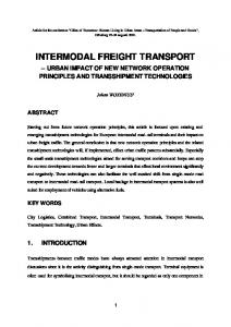
time based on infrastructure investment, the new container handling capacity and projected container volume through the facility would be useful. One problem an analyst will encounter is that the GIFT model cannot currently assign intermodal transfer times on a facility-by-facility basis. That is, changing the intermodal transfer time will affect all intermodal transfer facilities in the model. Therefore, if a route has more than one intermodal transfer, additional calculations outside of the GIFT model would have to be conducted to ensure a more accurate time-of-delivery for the route unless the analyst wishes to model a universal reduction in intermodal transfer times throughout the network. Consider Figure 14 below depicting the variables affecting intermodal transfer times. Containers enter the intermodal transfer facility via their respective spokes at a particular rate (containers/hr) indicated by “Rate of Incoming Container Offloading” and are stored on-site to await processing indicated by “Container Backlog at Intermodal Transfer Facility.” Containers are then loaded onto a truck, train, or ship according to the “Rate of Outgoing Container Loading” and depart the facility. Note that this is a simplified depiction of the process that I have created. Therefore, to reduce the intermodal transfer time for a container, infrastructure investments should affect the rate of incoming container offloading, the on-site capacity for container storage, or the rate of outgoing container loading (or a combination of these variables). It does no good to increase the ability of a facility to unload trucks, trains, and ships faster if they do not have the ability to store those containers. Also, if the rate of incoming container offloading is greater than the rate of outgoing container loading, there will not be a transfer time reduction. The analyst can use Figure 14 as a starting point to think about how various infrastructure investments would affect intermodal transfer times.
33
Truck Container Backlog at Intermodal Transfer Facility
Rail Ship
Truck Rail Ship
Rate of Incoming Container Offloading
Rate of Outgoing Container Loading
Figure 14 - Variables affecting intermodal transfer times.
6.3. Economic Incentives and Penalties Economic incentives and penalties include policies such as modal subsidies or grants, fuel taxes, carbon taxes, and CO2 cap-and-trade programs. 6.3.1. Modal Subsidies and Grants A modal subsidy or grant would affect the intermodalism/mode-shifting policy lever in the IF-TOLD framework by encouraging the use of less carbon-intense modes of freight transport. A subsidy or grant could be implemented through legislation and would make less carbon-intense modes of freight transport such as rail and ship less costly to use. It would be useful to have data on the costs and benefits, stakeholder views, and potential funding sources for the policy. Also, knowing which modes would be subsidized will be necessary. The costs of the policy might include the amount of money budgeted for the policy; the wages of the employees that would devise, implement, and evaluate the policy; economic loss to the trucking industry; and potential environmental and social costs from the increased use of rail and ship. The benefits of the policy might include the social and environmental benefits of reduced CO2 emissions and economic benefits to the rail and ship industries. Stakeholders would include policymakers, industry representatives, and the public. The policy would likely
34
result in an increased use of less carbon-intense modes of freight transport such as rail and ship and a decrease in the use of heavy-duty trucks. To model the impact of a modal subsidy or grant in the GIFT model, the analyst would adjust the per container-mile cost for each mode affected by the policy. For example, if the policy subsidized or offered grants to shippers who chose to transport their containers via rail or ship versus truck, then the analyst would take into consideration the cost-savings associated with the policy and reduce the per container-mile cost for the rail and ship segments of the network. Research would be necessary on the part of the analyst to find appropriate subsidy or grant levels. Freight modes like rail and ship are already less expensive than truck, so the point of the subsidy or grant is not to make the per container-mile cost of transporting goods by rail and ship less expensive than truck; rather, the point is to offset the other “costs” of transport by rail and ship. Specifically, as is shown in the case studies, rail and ship have a longer time-ofdelivery than truck; therefore, the analyst will need to determine what price per container-mile for rail and ship will offset the additional time-of-delivery for these modes. 6.3.2. Fuel Taxes A fuel tax based on carbon content would affect the “fuels” lever by making it more attractive to use low-carbon fuels. A fuel tax would also affect the “demand” lever by reducing demand for high-carbon fuels. A fuel tax could also affect the “technology” lever by encouraging companies to find and install fuel-saving technologies. The feasibility of implementing such a tax could be determined by collecting data on the costs and benefits and the stakeholder attitudes toward the policy. The costs of the policy might include increased economic cost to the truck, rail, and ship industries, increased cost to those industries‟ customers (the additional operating cost would likely be passed on), and economic
35
loss to oil companies due to decreased demand. The benefits of the policy might include reduced pollution and increased profit to alternative fuel suppliers and developers. The policy would likely result in an increased use of more fuel-efficient modes (like rail and ship versus truck) and a push toward technologies that improve fuel economy. To model the impact of a fuel tax in the GIFT model, the analyst would increase the per container-mile cost of each mode since operating costs would increase. To determine how much each mode‟s per container-mile cost should be increased, data on fuel economy would be necessary for the truck mode and data on energy use, horsepower, and service speed would be necessary for rail and ship. As a method of encouraging intermodalism/mode-shifting, a fuel tax would need to be high enough for shippers to be unwilling to use unimodal truck routes. The analyst would have to determine at what point a shipper would no longer use truck and make a switch to rail or ship. As discussed earlier, truck is already the most expensive mode of freight transport. Therefore, one of the reasons shippers use trucks is for their time-of-delivery advantage as well as their practicality for short-distance trips. The analyst should find a way to compare the tradeoffs associated with modal choice to better understand what it would take to influence intermodalism and mode-shifting. 6.3.3. Carbon Taxes A carbon tax based on the amount of CO2 emitted would affect the intermodalism/modeshifting, fuels, technology, operations, logistics, and demand levers. A carbon tax would incentivize a shift to less carbon intense modes of freight transport for all or part of the route, use of low carbon fuels, implementation of fuel efficient technologies, and better planning for
36
operating practices and logistics. A carbon tax would also reduce the demand for carbon-intense modes of freight transport and high-carbon fuels. Carbon dioxide emissions are a byproduct of diesel fuel combustion. The more fuel used, the greater the amount of CO2 emissions. In my research, I found that trucks emit the most amount of CO2 per container-mile compared to rail and ship. Trucks are also the most expensive mode of freight transport. Therefore, if a carbon tax is implemented, it will need to be high enough to discourage the use of unimodal truck routes in favor of intermodal routes or a modeshift to less carbon-intense modes (such as rail and ship). Like modeling a fuel tax, the analyst can increase the operating cost per container-mile for each mode in the GIFT model. The amount of the increase for each mode depends on the level of taxation for each unit of CO2 emitted (such as $/ton) and the efficiency of each mode. After applying the additional cost per container-mile, the analyst will notice that not much has changed. For example, truck will remain the fastest, but most expensive mode compared to rail and ship. The major tradeoff is in time-of-delivery. Therefore, the analyst needs to find a way to determine how much a shipper values time-of-delivery compared to operating costs. At a certain point, the shipper will find that it is not economically feasible to transport goods by carbonintense modes and will accept a slower time of delivery in order to reduce costs. 6.3.4. Cap-and-Trade Programs A cap-and-trade program would affect the intermodalism/mode-shifting, fuels, technology, operations, logistics, and demand levers. A cap-and-trade program would create an incentive to use low-carbon fuels, install technology to reduce fuel consumption and reduce CO 2 emissions, use best operating practices and adjust their supply chain to create efficiencies, and
37
create a demand for low-carbon fuels and technologies that reduce fuel consumption and CO 2 emissions. A cap-and-trade program would create a new market for tradable allowances. The allowances would essentially be the “right to pollute” by emitting CO 2. This would create an economic incentive to reduce CO2 emissions to similarly reduce the number of allowances that need to be purchased above the original allotment decided by policymakers. Also, if a company can reduce their emissions below their allotment, they would receive an economic benefit by selling their excess allowances to other firms. To determine the feasibility of such a policy, the costs and benefits and stakeholder views would need to be considered. The costs of a cap-and-trade program might include wages for employees to implement, administer, and evaluate the program, loss of revenue for oil companies from reduced sales of high-carbon fuels, and additional costs to firms above the established cap. The benefits of a cap-and-trade program might include reduced pollution, income from the sale of allowances by firms under the cap, investment in technologies that improve fuel efficiency, and investment in low-carbon fuels creating an economic boon to these industries. Stakeholders would likely include transportation industry representatives for each mode, oil companies, policymakers, federal and state agencies, and the public. The implementation of a cap-and-trade program might result in a shift toward less carbon-intense modes of freight transportation for intermodal and unimodal routes, investment in alternative fuels and fuel efficiency technologies, reduced demand for diesel fuel, and improved operations and logistics measures that promote efficiency. The GIFT model would be useful in determining baseline CO 2 emissions for each mode. If an industry-wide cap was implemented, the analyst would want to know how many trucks,
38
locomotives, and ships would be affected, and the fuel economy (for trucks) and energy use and horsepower (for rail and ship) of each vehicle being modeled. These estimates may have to be generated by a top-down approach to capture the characteristics of a typical truck, locomotive, or ship. As an example, assume that the cap-and-trade program aimed to reduce CO2 emissions by 50% compared to baseline truck emissions. If the analyst were modeling a trip from origin to destination, they could determine how much CO 2 would be emitted by a unimodal truck route. Then, they could try and find ways to reduce the amount of CO2 emitted by 50%. Methods to reduce CO2 emissions along that route could include increasing the truck‟s fuel economy or using a less carbon-intense mode for all or part of the route. Determining which method(s) achieve at least a 50% reduction of CO2 emissions helps predict what shippers might do to adjust to a cap-and-trade scenario. 6.4. Technology Implementation A policy could be implemented to require or incentivize the use of technologies that reduce emissions and improve fuel economy from freight transportation. Policies could be implemented through regulations or by providing subsidies or grants for their use. Examples of technologies that improve fuel efficiency could be low-rolling resistance tires and aerodynamic improvements for heavy duty diesel trucks (U.S. Environmental Protection Agency, 2009d). A technology implementation policy would affect the technology and demand levers. Mandating or incentivizing new technologies would create higher demand for those products. Data on the effectiveness of various technologies and their costs and benefits would be necessary in order to decide on the attractiveness of the policy. The costs of a technology implementation policy might include the price of the technology, wages for those who would administer and evaluate the policy, and reduced revenue for oil companies if the technologies
39
result in a net decrease in the amount of diesel fuel purchased. Benefits might include revenue for companies that produce the technologies, reduced pollution, and cost savings due to greater fuel economy. A technology implementation policy might result in lower CO 2 emissions due to reduced fuel consumption. To model the implementation of technologies that reduce fuel consumption in the GIFT model, the analyst would either adjust the amount of CO 2/TEU-mi for each mode or increase the mi/gal for trucks. Another way to model reduced fuel consumption would be to increase engine efficiencies for each mode in the Emissions Calculator. 6.5. The Benefits of Intermodalism and Mode-Shifting The policies described above can lead to intermodalism and mode-shifting. The benefits of intermodalism and mode-shifting include: (1) lower CO2 emissions; (2) lower economic costs; and (3) increased efficiency. Switching to intermodal routes that make use of less carbon-intense modes of freight transport (rail and ship) or switching from unimodal truck routes to unimodal rail and ship routes has the effect of reducing CO2 emissions. Reducing CO2 emissions results in lower social and environmental costs by reducing anthropogenic contributions to climate change. Lower CO2 emissions can also lead to cost savings if a “price for carbon” is implemented, such as a carbon tax or a cap-and-trade program for CO2 emissions; this results in a lower economic cost. Also, switching to intermodal or unimodal routes that use rail and ship are inherently less expensive due to increased efficiency, that is, more goods (by volume or weight) can be moved by rail and ship compared to truck at a lower price.
40
Switching to intermodal or unimodal routes that make use of rail and ship leads to greater efficiency. Increased fuel efficiency leads to lower fuel consumption and decreases our dependence on foreign oil. Thus, national security is improved as well. 6.6. Why Public Policies are Necessary to Reduce Freight Transport Energy Use and Emissions Public policies are necessary to reduce freight transport energy use and emissions in order to: (1) address a market failure; (2) provide economic security; and (3) improve national security. There is a market failure since social and environmental externalities are not included in freight transport costs (National Transport Commission & Rare Consulting, 2008). For example, the price of a gallon of diesel fuel does not account for the costs of environmental damage caused by the emissions generated from burning it (i.e. damage from acid deposition, contribution of CO2 to climate change, creation of ozone precursors, etc.) (Energy Information Administration, 2009b). Also, combustion of diesel fuel emits particulate matter and ozone precursors which can negatively impact human health. These costs are not captured in the market price. Polices that aim to reduce freight transport energy use and emissions can lead to the development of new technologies. These technologies can help drive a “green economy,” creating new jobs. Industry and shippers may claim that some policies would result in economic harm due to higher prices for transported goods. However, economic loss may be offset by increases in overall efficiency (i.e. transporting more goods using less energy and fuel), resulting in cost savings. Finally, much of our oil comes from unstable regions of the world, such as the Middle East, and threatens our national security. Policies that promote fuel efficient means of freight 41
transport reduce our dependence on foreign oil. By becoming more efficient and using less fossil fuel, or switching to domestically produced fuel (i.e. biodiesel, ethanol, natural gas, etc.), we rely less on foreign countries to support our freight transportation industry, an important piece of the U.S. economy. 7. Limitations of the Model and the Research 7.1. Speed Limits The first limitation relates to speed limits assigned to segments of the network. For the truck segments of the model, speed limits are assigned based on the road‟s classification. For example, every interstate on the network is assigned a speed of 65 miles per hour (mph), despite some interstates having a higher speed limit. For instance, portions of I-40 in New Mexico have a 75 mph speed limit. Therefore, routes that use the road network have a time-of-delivery based solely on the speed limit of the road (which may not reflect the actual speed limit) and does not take into consideration congestion. For the rail and ship segments of the network, the speed is a user input. A constant speed is applied to all segments of these networks. Therefore, the time-of-delivery for a route along the rail or ship networks is simply the distance divided by a constant speed. Thus, GIFT is currently incapable of modeling variable speeds along the rail and ship network which would make the model more accurate. The GIFT team is beginning to think about ways to adjust the model to reflect more realistic speeds for the rail and water networks of the model. One method being investigated for the water network is a buffer system. Buffers are applied within a certain distance from shore to model speed restrictions in near-shore areas. Other methods will be explored in the future.
42
7.2. Delays Delays are not well represented in the GIFT model. One delay that the GIFT team is working on integrating into the model is congestion delay along the road network. We are in the process of analyzing a new data set based on real-world GPS data. These data represent actual travel speeds along road segments and would better estimate actual time-of-delivery along the road network. Also, the road network does not consider delays associated with maximum allowable drive-hours for truckers. For example, a trucker may only be allowed to drive for 10 hours and then be required to rest for a specified amount of time before continuing. This delay would serve to increase the time-of-delivery associated with routes that contain segments of the road network. For the rail network, railyard dwell times are not accounted for within the GIFT model. The dwell time is the average time a rail car spends at a terminal before it is sent out to its destination ("Railroad performance measures: General definitions for measurements," 2009). The GIFT team is considering a buffer methodology to apply dwell times to the model. As an example, if a train comes within a certain distance of a railyard, an additional amount of time would be added to the overall time-of-delivery for the route to help model dwell times. For the water network, port and lock delays are not well represented. The papers found in Appendix A and Appendix B discuss the potential for lock delays to add a significant amount of time to overall time-of-delivery for routes on the Great Lakes. In order to capture lock delays, the analyst needs to decide how much time they want to add to time-of-delivery (based on the particular lock, average lock delay, and account for seasonality in that delay) outside of the GIFT model. Ideally, the GIFT model would account for lock delays endogenously. Finally variations in intermodal transfer times are applied uniformly to the network. Current transfer times are applied to intermodal spokes in the network and represent the physical 43
movement of a container from one mode to another, accounting for the fact that trains and ships carry multiple containers. The average intermodal transfer time includes not only the time it takes to move a container from one mode to another, but also the time a container waits to be moved from the initial mode to the second mode. This delay is different from a dwell time, which is a more systematic, logistically induced delay associated with the shipment of goods. For instance, a container on a train at a railyard, waiting to be affixed to a different locomotive, is experiencing a dwell time; a container on a train in queue to be transferred to another mode, is experiencing a transfer time. Even though railyards and ports have varying intermodal transfer times, the analyst can only choose one “representative” intermodal transfer time for each spoke (truck, rail, or ship). Thus, variations in intermodal transfer times cannot currently be modeled by the GIFT model. The GIFT team is working on finding realistic intermodal transfer times that can be used for representative spoke values in the network. This would make the model more accurate, but variable intermodal transfer times based on the attributes of the intermodal transfer facility would provide a more realistic representation of what actually occurs. 7.3. Energy Use and Emissions The aggregate energy use and emissions calculated by the model as a route traverses the network are based on user-defined assumptions. The vehicles modeled have a significant impact on the results of the total energy use and emissions reported by the GIFT model. Therefore, in analyzing the results of the case studies, it is important to realize that specific assumptions were made about the fuel economy, horsepower, container capacity, engine load factor, engine efficiency, and service speed of the vehicles being modeled. The GIFT team is constantly adding “predefined vehicles” to the dropdown menus in the Emissions Calculator. These vehicles can be chosen by an analyst or they can create their own vehicle profile.
44
Also, emissions are represented on a per mile basis. No consideration is given to changes in emissions as a function of speed, grade, or load. The GIFT team is researching how emissions change based on these variables and investigating ways to incorporate these variations into the model. If changes in emissions based on speed, grade, and load become endogenous to the GIFT model, the reported emissions for a route would better represent reality. Finally, emissions associated with intermodal transfers are a function of the amount and type of equipment used to transfer containers from one mode to another. The GIFT model assumes that the spokes attached to each intermodal facility emit the same amount of pollution at all intermodal facilities. Ideally, the GIFT model would know what equipment is used at each intermodal transfer facility and how much and what type of emissions they produce. Given that there are over 3,000 intermodal transfer facilities, this is not practical to do by hand. However, for smaller scale case studies, involving only a handful of intermodal transfer facilities, it may be possible to include a list of intermodal transfer equipment that an analyst can turn on and off. Thus, the analyst could pick and choose what equipment is actually used at the facility and obtain more realistic results. 7.4. Impacts of Limitations on Policy Research The model and research limitations discussed above can have a perverse influence on policy analysis related to freight transport. A key concern of shippers is time-of-delivery, so limitations related to speed and delay are important. Inaccurate travel speeds for truck, rail, and ship may impact policy analysis. For example, congestion increases the time-of-delivery along a route. This delay would be represented by a decrease in the speed of the truck, train, or ship along specific segments of the network. If the GIFT model were able to account for congestion, policy analysts would be able to conduct research on the impact of public policies aimed at
45
reducing congestion, and thereby reducing time-of-delivery. The analyst might perform a sensitivity analysis to determine how congestion impacts time-of-delivery and if that impact is significant. A sensitivity analysis could also be used when comparing the time-of-delivery across modes (i.e. the difference in time-of-delivery by truck compared to rail). One could hypothesize that delays such as congestion, dwell time, and intermodal transfer times, would have a proportional impact on overall time-of-delivery for a given route based on its overall length. That is, the same delay would represent a smaller percentage of overall time-of-delivery on a longer route (say from Los Angeles to Chicago) than a shorter route (say from Montreal to Cleveland). Therefore, performing a sensitivity analysis by altering delays along the route (perhaps by increasing and decreasing intermodal transfer times), may show the analyst which types of routes and flows should be targeted as suitable candidates for policy intervention. The potential for inaccurate energy use and emissions outputs from the GIFT model can also impact policy analysis. Not having emissions as a function of speed, grade, and load prevents micro-level policy analysis. That level of granularity may or may not be necessary to achieve broad policy conclusions. The impact of these limitations could be evaluated through sensitivity analysis. The analyst could change the assumptions of (1) the vehicles being modeled (horsepower, efficiency, engine load, container capacity, service speed) and (2) the equipment used at intermodal transfer facilities and their resulting emissions. Emissions are also a function of speed, grade, and load. Therefore, two routes that are the same distance, using the same modes, may not consume the same amount of energy or produce the same amount of emissions. This discrepancy is especially important when comparing the tradeoffs between modes. For example, a shipper may have a choice of shipping a container by train or by ship along the coast. If the two routes are similar in length, the GIFT model may indicate that the rail mode emits
46
slightly less emissions than the ship mode; however, if the train has to traverse mountains and travel at a high speed under heavy load, the reality may be that the train emits much more than the ship. Understanding the true tradeoffs between modal choices on these types of routes would enable to policymaker to make better decisions. 8. Conclusions My thesis focuses on the energy, environmental, and economic impacts and tradeoffs associated with freight transport. The case studies help quantify these impacts and tradeoffs. The results of the case studies make it clear that freight transport by heavy-duty trucks is less efficient than rail and ship based on CO2 emissions and operating costs, but more efficient based on time-of-delivery. Most U.S. freight is transported unimodally and is dominated by heavy-duty trucks. Trucks have been shown to be a carbon-intense mode of freight transport resulting in significant GHG emissions. Greenhouse gas emissions from the transportation sector are a major contributor to overall U.S. GHG emissions. While trucking has been the status quo for freight transport, I have shown that there are social, environmental, economic, and national security benefits to utilizing intermodal routes and shifting to less carbon-intense modes of freight transport. The GIFT model helps policy analysts quantify these benefits. One caveat is that the GIFT model contains limitations that need to be understood when interpreting the output and results from the model. In order to encourage a shift to more efficient modes of freight transport, public policies are necessary. Public policies are necessary in order to address market failures such as negative social and environmental externalities, promote economic growth, and improve national security by reducing our dependence on foreign oil. However, there are both costs and benefits to any
47
policy. The GIFT model can be useful in examining the impacts of public policy implementation and help the U.S. move toward a sustainable intermodal freight transport system. References Boile, M. P. (2000). Intermodal transportation network analysis - A GIS application. Paper presented at the 10th Mediterranean Electrotechnical Conference. Bureau of Economic Analysis (2007). National Income and Product Accounts Table Retrieved June 12, 2007, from http://www.bea.gov/bea/dn/nipaweb/index.asp Bureau of Transportation Statistics (2005). National Transportation Statistics 2005. Washington, DC: U.S. Department of Transportation, Research and Innovation Technology Administration. Bureau of Transportation Statistics (2007). Commodity Flow Survey. Washington, DC: Bureau of Transportation Statistics. Casgar, C. S., DeBoer, D. J., & Parkinson, D. L. (2003). Rail short haul intermodal corridor case studies: Industry context and issues: Foundation for Intermodal Research and Education (FIRE). Committee on the St. Lawrence Seaway (2008). Great Lakes Shipping, Trade, and Aquatic Invasive Species. Corbett, J. J., & Winebrake, J. J. (2007). Sustainable Movement of Goods: Energy and Environmental Implications of Trucks, Trains, Ships, and Planes. Environmental Management, November, 8-12. Corbett, J. J., & Winebrake, J. J. (2008). Emissions Tradeoffs among Alternate Marine Fuels: Total Fuel Cycle Analysis of Residual Oil, Marine Gas Oil, and Marine Diesel Oil. Journal of the Air & Waste Management Association, 58, 538-542. Corbett, J. J., Winebrake, J. J., Green, E. H., Kasibhatla, P., Eyring, V., & Lauer, A. (2007). Mortality from Ship Emissions: A Global Assessment. Environmental Science & Technology, 41(24), 8233-8239. Crainic, T. G. (2002). A survey of optimization models for long-haul freight transportation. Energy Information Administration (2009a). Annual Energy Outlook 2009 (No. DOE/EIA0383(2008)). Washington, DC: U.S. Department of Energy. Energy Information Administration (2009b). Diesel fuel explained: Diesel prices and outlook Retrieved November 20, 2009, from http://tonto.eia.doe.gov/energyexplained/index.cfm?page=diesel_prices Environmental Systems Research Institute (1992). Network Analysis Arc/INFO User's Guide 6.1. Falzarano, A. (2008). An evaluation of energy consumption and emissions from intermodal freight operations on the eastern seaboard: A GIS network analysis approach. Rochester Institute of Technology, Rochester, NY. Falzarano, A., Ketha, S., Winebrake, J. J., Hawker, J. S., Corbett, J. J., Korfmacher, K., et al. (2007). Development of an Intermodal Network for Freight Transportation Analysis. Paper presented at the ESRI International User Conference. Global Insight, & Reeve & Associates (2006). Four Corridor Case Studies of Short-Sea Shipping Services: U.S. Department of Transportation.
48
Great Lakes Feeder Lines (2008). Ship specs -- Dutch Runner Retrieved March 22, 2009, from http://www.glfl.ca/dutch-runner.html Great Lakes Maritime Taskforce (2007). Great Lakes Shipping Retrieved August 14, 2009, from http://www.glmtf.org/great_lakes_shipping.html Greening, L. A., Ting, M., & Davis, W. B. (1999). Decomposition of Aggregate Carbon Intensity for Freight: Trends from 10 OECD Countries for the Period 1971-1993. Energy Economics, 331-361. Hawker, J. S., Falzarano, A., Ketha, S., Korfmacher, K., Winebrake, J., & Zilora, S. (2007a). Intermodal Transportation Network Custom Evaluators for Environmental Policy Analysis. Paper presented at the ESRI International User Conference. Hawker, J. S., Falzarano, A., Ketha, S., Korfmacher, K., Winebrake, J. J., & Zilora, S. (2007b). Intermodal Transportation Network Custom Evaluators for Environmental Policy Analysis. Paper presented at the ESRI 2007 User Conference. Intergovernmental Panel on Climate Change (2007). Climate change 2007: synthesis report. New York. Luo, M., & Grigalunas, T. A. (2002). A multimodal transportation simulation model for US coastal container ports. Paper presented at the 2003 Transportation Research Board Conference. Midwest Regional University Transportation Center (2003). Twin Ports Intermodal Freight Terminal Study: Evaluation of Shipper Requirements and Potential Cargo Required to Establish a Rail-Truck-Marine Intermodal Terminal in the Twin Ports of Superior, Wisconsin and Duluth, Minnesota. Madison, Wisconsin: University of Wisconsin, Madison. National Ports and Waterways Institute (2004). The Public Benefits of the Short-Sea Intermodal System Retrieved March 30, 2006, from www.shortsea.us/benefits_study.pdf National Transport Commission, & Rare Consulting (2008). Freight transport in a carbon constrained economy. Melbourne, Australia. Office of Air Quality Planning and Standards (1994). Review of the National Ambient Air Quality Standards for sulfur oxides: Assessment of scientific and technical information. Research Triangle Park, NC. Owens, E., & Lewis, C. A. (2002). ISTEA and Intermodalism: A User and Reference Guide to Intermodalism (No. SWUTC/02/466050-1): Southwest Region University Transportation Center. Railroad performance measures: General definitions for measurements (2009). Retrieved November 20, 2009, from http://www.railroadpm.org/Definitions.aspx Ribeiro, S., Kobayashi, S., Beuthe, M., Gasca, J., Greene, D., Lee, D., et al. (2007). IPCC forth assessment report, working group III: Chapter 5, transportation and its infrastructure. Geneva, Switzerland: Intergovernmental Panel on Climate Change. Schipper, L., Scholl, L., & Price, L. (1997). Energy Use and Carbon Emissions from Freight in 10 Industrialized Countries: An Analysis of Trends from 1973 to 1992. Transportation Research Part D, 2(1), 57-76. Southworth, F., & Peterson, B. E. (2000). Intermodal and International Freight Network Modeling. In J.-C. Thill (Ed.), Geographic Information Systems in Transportation Research (pp. 147-166). Amsterdam, Netherlands: Pergamon Press Inc. St. Lawrence Seaway Management Corporation, & St. Lawrence Seaway Development Corporation (2008). The St. Lawrence Seaway traffic report: 2008 navigation season. 49
Standifer, G., & Walton, C. M. (2000). Development of a GIS model for intermodal freight. Austin, Texas: Southwest Regional University Transportation Center. Steenhof, P., Woudsma, C., & Sparling, E. (2006). Greenhouse Gas Emissions and the Surface Transport of Freight in Canada. Transportation Research Part D, 11, 369-376. TEMS Inc., & Rand Corporation (2007). Great Lakes-St. Lawrence Seaway new cargoes/new vessels market assessment report: MARAD. Transport Canada, US Army Corps of Engineers, US Department of Transportation, The St. Lawrence Seaway Management Corporation, Saint Lawrence Seaway Development Corporation, Environment Canada, et al. (2007). Great Lakes St. Lawrence Seaway Study. U.S. Energy Information Administration (2009). Annual energy outlook 2009 with projections to 2030. Washington, DC: U.S. Department of Energy. U.S. Environmental Protection Agency (2006a). Greenhouse gas emissions from the U.S. transportation sector 1990-2003. U.S. Environmental Protection Agency (2006b). U.S. Greenhouse Gas Inventory Report, Annex 2 (No. USEPA #430-R-06-002). Washington, DC. U.S. Environmental Protection Agency (2008). Inventory of U.S. greenhouse gas emissions and sinks: 1990-2006. Washington, DC. U.S. Environmental Protection Agency (2009a). Acid rain: Effects of acid rain Retrieved November 17, 2009, from http://www.epa.gov/acidrain/effects/index.html U.S. Environmental Protection Agency (2009b). Acid rain: Reducing acid rain Retrieved November, 17, 2009, from http://www.epa.gov/acidrain/reducing/index.html U.S. Environmental Protection Agency (2009c). Clean air research program: Particulate matter (PM) basics Retrieved November 17, 2009, from http://www.epa.gov/airscience/quickfinder/particulate-matter.htm#4 U.S. Environmental Protection Agency (2009d). EPA releases SmartWay SIP and transportation conformity guidance: Accounting for NOx reductions from trailer aerodynamic kits and low-rolling resistance tires Retrieved November 21, 2009, from http://www.epa.gov/OMSWWW/stateresources/transconf/policy/420f07045.htm U.S. Environmental Protection Agency (2009e). Ground-level ozone: Health and environment Retrieved November 17, from http://www.epa.gov/air/ozonepollution/health.html U.S. Environmental Protection Agency (2009f). Inventory of U.S. Greenhouse Gas Emissions and Sinks: 1990-2007 (No. USEPA #430-R-07-002). Washington, DC. U.S. Environmental Protection Agency (2009g). Sulfur dioxide: Health Retrieved November 17, 2009, from http://www.epa.gov/air/sulfurdioxide/health.html Vanek, F. M., & Morlok, E. K. (2000). Improving the Energy Efficiency of Freight in the United States Through Commodity-Based Analysis: Justification and Implementation. Transportation Research Part D, 5(1), 11-29. Wang, C., Corbett, J. J., & Winebrake, J. J. (2007). Cost Effectiveness of Reducing Ship Sulfur Emissions. Environmental Science & Technology, 41(25). Winebrake, J. J. (2009). Improving the energy efficiency and environmental performance of goods movement. Paper presented at the Conference on Transportation and Energy, Asilomar. Winebrake, J. J., Corbett, J. J., Falzarano, A., Hawker, J. S., Korfmacher, K., Ketha, S., et al. (2008a). Assessing Energy, Environmental, and Economic Tradeoffs in Intermodal Freight Transportation Journal of the Air & Waste Management Association, 58(8). 50
Winebrake, J. J., Corbett, J. J., Hawker, J. S., Korfmacher, K., Comer, B., & Prokop, C. (2008b). Intermodal freight transport in the Great Lakes: Development and application of a Great Lakes geographic intermodal freight transport model. Winebrake, J. J., Corbett, J. J., & Meyer, P. (2007a). Energy Use and Emissions from Marine Vessels: A Total Fuel Life Cycle Approach. Journal of the Air and Waste Management Association, 57, 102-110. Winebrake, J. J., Corbett, J. J., & Meyer, P. E. (2007b). Energy Use and Emissions from Marine Vessels: A Total Fuel Cycle Approach. Journal of Air and Waste Management, 57(January), 102-110. Zhan, F. B. (1997). Three fastest shortest path algorithms on real road networks: Data structures and procedures. Journal of Geographic Information and Decision Analysis, 1(1), 69-82.
51
Appendix A
A-1
MARINE VESSELS AS SUBSTITUTES FOR HEAVY-DUTY TRUCKS IN GREAT LAKES FREIGHT TRANSPORTATION Bryan Comer, Rochester Institute of Technology James J. Corbett, University of Delaware J. Scott Hawker, Rochester Institute of Technology Karl Korfmacher, Rochester Institute of Technology Earl E. Lee, University of Delaware Chris Prokop, Rochester Institute of Technology James J. Winebrake, Rochester Institute of Technology (corresponding author) ABSTRACT This paper applies a geospatial network optimization model to explore environmental, economic, and time-of-delivery tradeoffs associated with the application of marine vessels as substitutes for heavy-duty trucks operating in the Great Lakes region. The geospatial model integrates U.S. and Canadian highway, rail, and waterway networks to create an intermodal network and characterizes this network using temporal, economic, and environmental attributes (including emissions of carbon dioxide, particulate matter, carbon monoxide, sulfur oxides, volatile organic compounds, and nitrogen oxides). A case study evaluates tradeoffs associated with containerized traffic flow in the Great Lakes region, demonstrating how modal choice affects the environmental performance of goods movement. These results suggest opportunities to improve the environmental performance of freight transport through infrastructure development, technology implementation, and economic incentives. 1.
INTRODUCTION Energy use and emissions from freight transport are increasing at a more rapid rate than other types of transportation (Corbett & Winebrake, 2007; Energy Information Administration, 2009a), and freight transport represents a non-negligible component of local air pollution and greenhouse gases (GHG) (Corbett & Winebrake, 2008; Corbett, et al., 2007; Wang, Corbett, & Winebrake, 2007; Winebrake, Corbett, & Meyer, 2007a). One way to address these growing impacts is through careful consideration of routes along an intermodal freight system (Owens & Lewis, 2002; Winebrake, et al., 2008a). Route selection based on environmental criteria, as opposed to the traditional criteria of cost and time-of-delivery, could help identify environmentally-sustainable ways to move freight throughout the U.S. and abroad (Winebrake, et al., 2008a). This paper applies the Geospatial Intermodal Freight Transport (GIFT) model discussed in Winebrake et al. (2008) to evaluate environmental, economic cost, and time-of-delivery tradeoffs associated with containerized freight transport in the Great Lakes region of North America. GIFT consists of an intermodal (rail, highway, and waterway) network that is characterized not only by distance and time-of-delivery, but also by operating costs, energy (Btu), and emissions [carbon dioxide (CO2), carbon monoxide (CO), particulate matter (PM10), nitrogen oxides (NOx), volatile organic compounds (VOC), and sulfur oxides (SOx)] (Falzarano, et al., 2007; Hawker, et al., 2007b). For this paper, GIFT has been expanded to include integration of U.S. and Canadian road, rail, and water networks and has been improved via the use of a „hub-and-spoke‟ intermodal connection feature. Here, GIFT is applied to examine the
A-2
tradeoffs associated with a shift from heavy-duty trucks to ships for freight transport in the Great Lakes region. 2.
BACKGROUND
2.1 Energy and Environmental Impacts of Freight Transport The growing literature surrounding the important role that freight transportation plays in economic development has also highlighted the increasing energy and environmental impacts associated with cargo movement (Corbett & Winebrake, 2007; Corbett & Winebrake, 2008; Corbett, et al., 2007; Greening, Ting, & Davis, 1999; Schipper, Scholl, & Price, 1997; Vanek & Morlok, 2000; Winebrake, et al., 2008a; Winebrake, Corbett, & Meyer, 2007b). For example, the U.S. spends about 6-7% of its GDP on freight transport annually, and U.S. reliance on the freight transportation system has been growing considerably for some time (Bureau of Economic Analysis, 2007; Bureau of Transportation Statistics, 2005). Notwithstanding the recent decline in goods movement due to negative economic growth in 2008, long-term trends of U.S. domestic ton-miles of goods transported via multiple modes have steadily increased (Bureau of Transportation Statistics, 2005, 2007). For instance, under its reference case scenario, the U.S. Energy Information Administration (EIA) projects total vehicle miles traveled (VMT) for freight trucking to increase from 224 billion VMT to 378 billion VMT between 2006 and 2030, an average annual increase of 1.9%. Likewise, rail freight transport is expected to increase from about 1,718 billion ton-miles (BTM) to 2,193 BTM (1.0%/yr) over the same period, while domestic marine freight is expected to increase from 659 BTM to 839 BTM (1.0%/yr). Finally, air freight transport is expected to increase from 37 BTM to 84 BTM (3.5%/yr) (U.S. Energy Information Administration, 2009). With increasing freight transport activity and accompanying energy use, GHG emissions will also increase. In 2007, freight transport (including rail, truck, air, and domestic shipping) was responsible for about 660 teragrams of CO2 (Tg CO2) in the U.S., or about 9% of total CO2 emissions1 (U.S. Environmental Protection Agency, 2009f). This is consistent with other industrialized countries, such as Canada where freight transport represents about 9% of total GHG emissions (Steenhof, Woudsma, & Sparling, 2006). Responding to the idea that mode shifts can help achieve reduction targets for energy and emissions (Ribeiro, et al., 2007), this paper examines the potential for freight emissions reduction, particularly of CO2, through a shift from carbon-intense modes of freight transport (trucks) to a less carbon-intense mode (marine vessels) in the Great Lakes region. 3.
FREIGHT TRANSPORT IN THE GREAT LAKES REGION The Great Lakes Region includes the entire St. Lawrence Seaway System (SLSS), which extends as far east as the Gulf of St. Lawrence and as far west as the Port of Duluth, encompassing all five major Laurentian Great Lakes (Ontario, Erie, Huron, Michigan, and Superior) (Committee on the St. Lawrence Seaway, 2008). This region is home to approximately 10% and 30% of the populations of the U.S. and Canada, respectively. The region is considered one of “the world‟s largest manufacturing and consumer markets” (TEMS Inc. & Rand Corporation, 2007), and is a critical artery of commerce for the U.S. The Great Lakes region also plays a key role in international trade with goods entering the St. Lawrence 1
Derived from Tables 2-12 and 2-15 of EPA‟s Inventory of U.S. Greenhouse Gas Emissions and Sinks: 1990-2007,
A-3
Seaway from the Atlantic Ocean and goods entering from the west at ports such as Duluth and Thunder Bay, Minnesota (TEMS Inc. & Rand Corporation, 2007). In 2008, approximately 114 million short tons of cargo were transported on the Great Lakes (St. Lawrence Seaway Management Corporation & St. Lawrence Seaway Development Corporation, 2008). The majority of waterborne cargo in the Great Lakes is carried by a fleet of dry-bulk cargo ships and “self-unloaders”. The latter type of ship is essentially a dry-bulk carrier with integrated lifts and conveyors to facilitate unloading without extensive shore-side infrastructure (Great Lakes Maritime Taskforce, 2007). Tug boats are often used to push a small number of barges, which can be used on the lakes as well as on most of the waterways that communicate with the Great Lakes. Increasingly, integrated tug-barge combination ships are being used in which the flat area of the barge is included in an extended section of the tug boat hull (TEMS Inc. & Rand Corporation, 2007). Notably absent from the discussion of Great Lakes waterborne freight traffic is containerization, which is currently a negligible component of Great Lakes shipping (with the exception of some regular activity at the Port of Montreal associated with trans-Atlantic shipments). Currently, almost all containerized freight in the region is carried by land-based modes of transportation, often by heavy-duty diesel trucks. However, there appears to be interest and room for growth for on-water, containerized freight transport in order to reduce highway and rail congestion in the Great Lakes region. One estimate suggests that on-water goods movement could capture as much as four percent of containerized intermodal traffic in the Great Lakes region by 2050 so long as it is competitive with truck and rail (TEMS Inc. & Rand Corporation, 2007). This waterborne activity would work in conjunction with land-side modes using intermodal freight transportation facilities to enable modal transfers if necessary. Our case study examines the potential benefits of on-water containerized freight in the Great Lakes region. 4.
MODELING APPROACH In this paper, the GIFT model is used to evaluate the economic cost, time-of-delivery, and environmental impacts associated with modal choices of freight transport (by truck, rail, or ship). GIFT is a network optimization model that operates on an ArcGIS 9.3 software platform. The model applies the shortest path algorithm included in ArcGIS‟s Network Analyst to evaluate U.S. and Canadian freight movements from origin to destination. GIFT includes two unique elements that make it useful for evaluating intermodal shipments. First, GIFT includes an intermodal network that links publicly available U.S. and Canadian, unimodal network datasets (currently rail, highway, and waterway) through nodes identified at ports, railyards, and other intermodal facilities. This allows the user to model the transfer of goods from one mode to another. Second, GIFT includes energy, environmental, economic, and speed attribute information (by mode) on each segment and node of the intermodal network. Attributes such as emissions of various pollutants (e.g., CO2, PM10 , NOx, SOx, and VOCs), energy consumption (e.g., Btu), time, and economics ($) have been incorporated into GIFT. This feature allows the analyst to solve the network transportation problem for different objective functions, such as least time, least cost, and least emissions. The GIFT model has been discussed in detail in previous work (Falzarano, et al., 2007; Hawker, et al., 2007a; Winebrake, et al., 2008a) and we refer the reader to that literature for details about model development. By analyzing the network using energy and environmental objective functions, tradeoffs among these goals and more traditional ones (cost and time-of-delivery) can be explored. Policy A-4
analysis can also be studied to determine how such policies (e.g., modal taxes, low carbon fuel mandates, or subsidies) would affect the overall energy and environmental character of freight transport. In this paper, tradeoffs associated with modal choice are examined with particular focus on time-of-delivery, CO2 emissions, and operating cost. 5.
A GREAT LAKES CASE STUDY We present a case study representing a containerized cargo flow scenario found in the Great Lakes-St. Lawrence Seaway New Cargoes/New Vessels Market Assessment Report (TEMS Inc. & Rand Corporation, 2007). This case involves moving containerized goods from Montreal, Canada to Cleveland, Ohio, USA. We evaluate a shipment of goods along this route under different objectives and shipping options, including the following modal assumptions: Truck – a model year 2007 or later (MY2007+) Class 8 tractor trailer able to haul two twenty-foot equivalent unit (TEU) containers at seven tons per TEU. We assume this truck has a fuel economy of 6 miles per gallon when loaded. Rail – two Tier 2 4,000 horsepower (hp) locomotives (2005 or later build date) pulling 100 wells with 4 TEUs per well (400 TEUs total, or 3,200 tons) (Casgar, DeBoer, & Parkinson, 2003). We assume these engines operate at 35% efficiency with an average load factor of 70%. Ship #1 – a 221 TEU capacity, 3,071 hp container vessel called the Dutch Runner (1988 build date) (Great Lakes Feeder Lines, 2008). We assume the engine operates at 40% efficiency with an average load factor of 80%. Ship #2 – a 200 TEU capacity, 1,550 hp tug-barge combination vessel called the Ellie J. (1968 build date, 2007 rebuild date). We assume the engine operates at 40% efficiency with an average load factor of 65%. Fuel – the assumed fuel for this case is on-road diesel fuel with energy content of 128,450 Btu/gallon, a mass density of 3,170 grams/gallon, and a carbon fraction of 86%. We calculate emissions factors for each mode on a per TEU basis, as shown in the Appendix. We also apply “penalties” within GIFT for intermodal transfers accounting for additional time, costs, and emissions from such transfers. We estimate emissions from transfer activities for each of the three spokes (rail-, truck-, ship-to-hub) using an activity based model called the “Container Transfer Emissions Model” (CTEM). CTEM identifies the different pieces of equipment used to move containers from one mode to another, applies temporal and engine load factors for such transfers, and applies emissions factors from the California Air Resource Board‟s (CARB) OFFROAD model for each piece of equipment to estimate actual emissions for mode-to-mode transfers. The two ships modeled in this paper are assumed to use all port-side transfer equipment included in the CTEM. Based on CTEM, we calculate truck-to-ship, truckto-rail, and rail-to-ship emissions factors of 11.7, 13.3, and 6.6 kg CO 2/TEU, respectively. Modal operating costs for each segment were derived from the Four Corridor Case Studies of Short-Sea Shipping Services prepared by Global Insight 2 (2006). The cost data used in this analysis are: $0.87/TEU-mile for truck; $0.55/TEU-mile for rail; and $0.50/TEU-mile for ship. Intermodal transfer costs were obtained from a report on short-sea shipping and are a sum of the port cost and the local drayage costs outlined in that report (Midwest Regional University Transportation Center, 2003). We assume a cost of $70/TEU for each mode-to-mode transfer. 2
See table IV-3 of the referenced report.
A-5
To calculate time-of-delivery for a given route, we sum the travel time on each segment of the route and the time it takes to transfer between modes (if such transfers take place). For our segment time, we use reported speed limits for truck, average speed for rail, and ship service speed for ship. The speed we use for rail segments is 25 mph.3 The two speeds we use for the ship segments are 13.5 mph and 9 mph corresponding to design speeds for the Dutch Runner and the Ellie J., respectively. We use a two hour penalty for each intermodal transfer. 6.
RESULTS The case study examines the CO2 emissions, time-of-delivery, and operating cost tradeoffs of freight transport according to modal choice. We compare the truck, rail, and shipping options presented above, using an origin of Montreal and a destination of Cleveland. The model is run three times under the following objective functions: (1) least time; (2) least CO2; and (3) least cost. Figure 1 shows the results of the analysis based on (a) the Dutch Runner case, and (b) the Ellie J. case. Table 1 shows the results of each model run. These results are depicted graphically in Figure 2. Figure 1: (a) Results of Montreal-to-Cleveland case where the ship is the Dutch Runner container vessel (left); (b) Results of the Montreal-to-Cleveland case where the ship is the Ellie J. tug-and-barge vessel (right).
3
This value is within the reported average operating speeds of freight locomotives as reported at http://www.railroadpm.com which reports railroad performance measures.
A-6
Table 1: Results for Three Optimization Model Runs from Montreal to Cleveland.
Case Objective (a) Least Time Dutch Runner Least Cost container vessel Least CO2 (b) Least Time Ellie J. tugLeast Cost and-barge Least CO2
Primary Mode Truck Ship Rail Truck Ship Ship
Total CO2 (kg/TEU) 460 240 190 460 160 160
A-7
Total Time (hrs) 8 42 25 8 60 60
Total Distance (miles) 552 517 532 552 503 503
Total Cost ($/TEU) 480 400 430 480 420 420
Figure 2. Results for the Montreal-to-Cleveland route based on (a) least-CO2 objective function (top); (b) least-cost objective function (middle); and (c) least-time objective function (bottom).
The most carbon-intensive mode of freight transport in this case is truck, followed by the container ship (the Dutch Runner), rail, and the tug-and-barge vessel (the Ellie J.). The Ellie J. performs the best with respect to CO2 emissions. The two marine vessels are the best choice when the objective is to minimize operating costs; however, the emissions and economic benefits come at a time-of-delivery penalty. Note that the time-of-delivery presented does not include A-8
delays due to congestion or border crossing for any of the modes, or lock delays for ships. This functionality is currently being developed within GIFT. One important outcome of these results is the relative importance of modal characteristics as they pertain to CO2 emissions. In particular, engine horsepower, cargo capacity, engine type, and speed all affect CO2 emissions. CO2 emissions for the Dutch Runner, rail, and Ellie J. perform similarly and are around 1/3 to 1/2 the emissions from truck. Truck remains the most expensive mode of freight transport in the Great Lakes region under published rate comparisons, and rail and ship may compete to be the cheapest mode, depending on the other service requirements imposed on these modes. In addition, our origin and destination are located on truck delivery segments. If a facility at the origin or destination can directly load cargo onto ship or rail, transfer penalties associated with this routing may be reduced. 7.
CONCLUSION Discussions of the competitiveness of rail and ship compared to trucks require understanding the tradeoffs associated with any mode that is chosen. Trucks are often the fastest way to move containers but emit the greatest amount of CO 2. Ships are often the cheapest way to move containers but have a relatively longer time-of-delivery, and some ships offer lowest CO2 alternative at less cost than trucking. Environmental policy incentives to make ships more attractive and competitive with trucks must consider multiple performance metrics (e.g., not just time of travel) to incentivize freight transportation in the Great Lakes region by ship. Some policies that could make ships a more attractive mode of freight transportation include infrastructure development, technology implementation, and economic incentives. Policymakers can use GIFT to test the impacts of carbon taxes, fuel taxes, or modal subsidies by adjusting costs in GIFT and observing the routing impacts due to these economic instruments. Policymakers could also modify emissions factors or energy consumption to simulate the impact of new emissions control technologies or fuel efficiency mandates. For example, to incentivize a shift to marine based freight transport in the Great Lakes, policies could include a carbon tax, port and lock infrastructure improvement and development, and modal subsidies and grants. A carbon tax would increase the cost of shipping freight by truck due to its carbon-intensity. At some price for carbon, less carbon-intense modes like ships would become more attractive. Port and lock infrastructure improvement and development would allow for more opportunities for container vessels to operate on the Great Lakes as well as reduce lock delays in order to reduce time-of-delivery. Modal subsidies and grants for shippers who switch from truck to ship would provide an economic incentive to utilize the Great Lakes as a freight transport corridor. Though transporting freight by ship will be slower than truck, the economic savings may help balance the “cost” of a longer time-of-delivery. 8.
ACKNOWLEDGEMENTS Partial support of this research was provided by the Great Lakes Maritime Research Institute and the U.S. Department of Transportation Maritime Administration. The authors are solely responsible for all views expressed in this paper.
A-9
REFERENCES Boile, M. P. (2000). Intermodal transportation network analysis - A GIS application. Paper presented at the 10th Mediterranean Electrotechnical Conference. Bureau of Economic Analysis (2007). National Income and Product Accounts Table Retrieved June 12, 2007, from http://www.bea.gov/bea/dn/nipaweb/index.asp Bureau of Transportation Statistics (2005). National Transportation Statistics 2005. Washington, DC: U.S. Department of Transportation, Research and Innovation Technology Administration. Bureau of Transportation Statistics (2007). Commodity Flow Survey. Washington, DC: Bureau of Transportation Statistics. Casgar, C. S., DeBoer, D. J., & Parkinson, D. L. (2003). Rail short haul intermodal corridor case studies: Industry context and issues: Foundation for Intermodal Research and Education (FIRE). Committee on the St. Lawrence Seaway (2008). Great Lakes Shipping, Trade, and Aquatic Invasive Species. Corbett, J. J., & Winebrake, J. J. (2007a). Sustainable Movement of Goods: Energy and Environmental Implications of Trucks, Trains, Ships, and Planes. Environmental Management, November. Corbett, J. J., & Winebrake, J. J. (2007b). Sustainable Movement of Goods: Energy and Environmental Implications of Trucks, Trains, Ships, and Planes. Environmental Management, November, 8-12. Corbett, J. J., & Winebrake, J. J. (2008). Emissions Tradeoffs among Alternate Marine Fuels: Total Fuel Cycle Analysis of Residual Oil, Marine Gas Oil, and Marine Diesel Oil. Journal of the Air & Waste Management Association, 58, 538-542. Corbett, J. J., Winebrake, J. J., Green, E. H., Kasibhatla, P., Eyring, V., & Lauer, A. (2007). Mortality from Ship Emissions: A Global Assessment. Environmental Science & Technology, 41(24), 8233-8239. Crainic, T. G. (2002). A survey of optimization models for long-haul freight transportation. Energy Information Administration (2009). Annual Energy Outlook 2009 (No. DOE/EIA0383(2008)). Washington, DC: U.S. Department of Energy. Environmental Systems Research Institute (1992). Network Analysis Arc/INFO User's Guide 6.1. Falzarano, A. (2008). An evaluation of energy consumption and emissions from intermodal freight operations on the eastern seaboard: A GIS network analysis approach. Rochester Institute of Technology, Rochester, NY. Falzarano, A., Ketha, S., Winebrake, J. J., Hawker, J. S., Corbett, J. J., Korfmacher, K., et al. (2007). Development of an Intermodal Network for Freight Transportation Analysis. Paper presented at the ESRI International User Conference. Global Insight, & Reeve & Associates (2006). Four Corridor Case Studies of Short-Sea Shipping Services: U.S. Department of Transportation. Great Lakes Feeder Lines (2008). Ship specs -- Dutch Runner Retrieved March 22, 2009, from http://www.glfl.ca/dutch-runner.html Great Lakes Maritime Taskforce (2007). Great Lakes Shipping Retrieved August 14, 2009, from http://www.glmtf.org/great_lakes_shipping.html
A-10
Greening, L. A., Ting, M., & Davis, W. B. (1999). Decomposition of Aggregate Carbon Intensity for Freight: Trends from 10 OECD Countries for the Period 1971-1993. Energy Economics, 331-361. Hawker, J. S., Falzarano, A., Ketha, S., Korfmacher, K., Winebrake, J., & Zilora, S. (2007). Intermodal Transportation Network Custom Evaluators for Environmental Policy Analysis. Paper presented at the ESRI International User Conference. Hawker, J. S., Falzarano, A., Ketha, S., Korfmacher, K., Winebrake, J. J., & Zilora, S. (2007). Intermodal Transportation Network Custom Evaluators for Environmental Policy Analysis. Paper presented at the ESRI 2007 User Conference. Luo, M., & Grigalunas, T. A. (2002). A multimodal transportation simulation model for US coastal container ports. Paper presented at the 2003 Transportation Research Board Conference. Midwest Regional University Transportation Center (2003). Twin Ports Intermodal Freight Terminal Study: Evaluation of Shipper Requirements and Potential Cargo Required to Establish a Rail-Truck-Marine Intermodal Terminal in the Twin Ports of Superior, Wisconsin and Duluth, Minnesota. Madison, Wisconsin: University of Wisconsin, Madison. National Ports and Waterways Institute (2004). The Public Benefits of the Short-Sea Intermodal System Retrieved March 30, 2006, from www.shortsea.us/benefits_study.pdf Owens, E., & Lewis, C. A. (2002). ISTEA and Intermodalism: A User and Reference Guide to Intermodalism (No. SWUTC/02/466050-1): Southwest Region University Transportation Center. Ribeiro, S., Kobayashi, S., Beuthe, M., Gasca, J., Greene, D., Lee, D., et al. (2007). IPCC forth assessment report, working group III: Chapter 5, transportation and its infrastructure. Geneva, Switzerland: Intergovernmental Panel on Climate Change. Schipper, L., Scholl, L., & Price, L. (1997). Energy Use and Carbon Emissions from Freight in 10 Industrialized Countries: An Analysis of Trends from 1973 to 1992. Transportation Research Part D, 2(1), 57-76. Southworth, F., & Peterson, B. E. (2000). Intermodal and International Freight Network Modeling. In J.-C. Thill (Ed.), Geographic Information Systems in Transportation Research (pp. 147-166). Amsterdam, Netherlands: Pergamon Press Inc. St. Lawrence Seaway Management Corporation, & St. Lawrence Seaway Development Corporation (2008). The St. Lawrence Seaway traffic report: 2008 navigation season. Standifer, G., & Walton, C. M. (2000). Development of a GIS model for intermodal freight. Austin, Texas: Southwest Regional University Transportation Center. Steenhof, P., Woudsma, C., & Sparling, E. (2006). Greenhouse Gas Emissions and the Surface Transport of Freight in Canada. Transportation Research Part D, 11, 369-376. TEMS Inc., & Rand Corporation (2007). Great Lakes-St. Lawrence Seaway new cargoes/new vessels market assessment report: MARAD. Transport Canada, US Army Corps of Engineers, US Department of Transportation, The St. Lawrence Seaway Management Corporation, Saint Lawrence Seaway Development Corporation, Environment Canada, et al. (2007). Great Lakes St. Lawrence Seaway Study. U.S. Energy Information Administration (2007). Annual Energy Outlook 2007 with Projections to 2030 (No. DOE/EIA-0383). Washington, DC: U.S. Department of Energy.
A-11
U.S. Energy Information Administration (2009). Annual energy outlook 2009 with projections to 2030. Washington, DC: U.S. Department of Energy. U.S. Environmental Protection Agency (2006a). Greenhouse gas emissions from the U.S. transportation sector 1990-2003. U.S. Environmental Protection Agency (2006b). U.S. Greenhouse Gas Inventory Report, Annex 2 (No. USEPA #430-R-06-002). Washington, DC. U.S. Environmental Protection Agency (2008). Inventory of U.S. greenhouse gas emissions and sinks: 1990-2006. Washington, DC. U.S. Environmental Protection Agency (2009). Inventory of U.S. Greenhouse Gas Emissions and Sinks: 1990-2007 (No. USEPA #430-R-07-002). Washington, DC. Vanek, F. M., & Morlok, E. K. (2000). Improving the Energy Efficiency of Freight in the United States Through Commodity-Based Analysis: Justification and Implementation. Transportation Research Part D, 5(1), 11-29. Wang, C., Corbett, J. J., & Winebrake, J. J. (2007). Cost Effectiveness of Reducing Ship Sulfur Emissions. Environmental Science & Technology, 41(25). Winebrake, J. J., Corbett, J. J., Falzarano, A., Hawker, J. S., Korfmacher, K., Ketha, S., et al. (2008). Assessing Energy, Environmental, and Economic Tradeoffs in Intermodal Freight Transportation Journal of the Air & Waste Management Association, 58(8). Winebrake, J. J., Corbett, J. J., & Meyer, P. (2007). Energy Use and Emissions from Marine Vessels: A Total Fuel Life Cycle Approach. Journal of the Air and Waste Management Association, 57, 102-110. Winebrake, J. J., Corbett, J. J., & Meyer, P. E. (2007). Energy Use and Emissions from Marine Vessels: A Total Fuel Cycle Approach. Journal of Air and Waste Management, 57(January), 102-110. Zhan, F. B. (1997). Three fastest shortest path algorithms on real road networks: Data structures and procedures. Journal of Geographic Information and Decision Analysis, 1(1), 69-82.
A-12
Appendix B
B-1
SUSTAINABLE INTERMODAL FREIGHT TRANSPORTATION: USING GREAT LAKES SHORT-SEA SHIPPING ALONG AN INTERMODAL ROUTE Bryan Comer, Rochester Institute of Technology James J. Winebrake, Rochester Institute of Technology J. Scott Hawker, Rochester Institute of Technology Karl Korfmacher, Rochester Institute of Technology Chris Prokop, Rochester Institute of Technology James J. Corbett, University of Delaware ABSTRACT This paper applies a geospatial network optimization model to explore environmental, economic, and time-of-delivery tradeoffs associated with intermodal freight transportation. The geospatial model integrates U.S. and Canadian highway, rail, and waterway networks to build an intermodal network and characterizes this network using temporal, economic, and environmental attributes (including emissions of carbon dioxide, particulate matter, carbon monoxide, sulfur oxides, volatile organic compounds, and nitrogen oxides). This paper applies the model in a case study to evaluate tradeoffs associated with unimodal and intermodal freight transport for the motorized vehicle sector. Geographically, this paper focuses on freight routes that traverse the Great Lakes region; however, the origin and destination need not be in the Great Lakes region itself. The paper demonstrates the potential benefits of using the Great Lakes as a corridor for intermodal freight transportation of motorized vehicles and their parts and suggests opportunities to this use through infrastructure development, technology implementation, and economic incentives. 1.
INTRODUCTION Energy use and emissions from freight transport are increasing at a more rapid rate than other types of transportation (Corbett & Winebrake, 2007; Energy Information Administration, 2009a), and freight transport represents a non-negligible component of local air pollutants and greenhouse gases (GHG) (Corbett & Winebrake, 2008; Corbett, et al., 2007; Wang, et al., 2007; Winebrake, et al., 2007a). One way to address these growing impacts is through careful consideration of routes along an intermodal freight system (Owens & Lewis, 2002; Winebrake, et al., 2008a). Route selection based on environmental criteria, as opposed to the traditional criteria of cost and timeof-delivery, could help identify environmentally-sustainable ways to move freight throughout the U.S. and abroad (Winebrake, et al., 2008a). This paper applies the Geospatial Intermodal Freight Transport (GIFT) model discussed in Winebrake et al. (2008) to evaluate environmental, cost, and time-of-delivery tradeoffs associated with unimodal versus intermodal freight transport. Specifically, we focus on using the Great Lakes as a corridor for intermodal freight transportation in the motorized vehicle sector. We use the definition of “motorized and other vehicles” from the 2002 Commodity Flow Survey. The “motorized and other vehicles” category includes passenger vehicles and their parts, such as brakes, gear boxes, road wheels, bumpers, etc. We chose this sector since 98% of motorized vehicles and their parts are shipped by truck in the Great Lakes region (see Figure ). B-2
Therefore, there is an opportunity for modal shifting from truck to other modes, including intermodal routes.
Modal Share of Motorized Vehicle Freight Transport, 2002 (kTon) Truck & Rail Rail Water 1% 0% Air & Truck 0% Unknown 0% 1%
Truck 98% Figure 1: Modal share of motorized vehicle freight transport, 2002 (kTon)
GIFT consists of an intermodal (rail, highway, and waterway) network that is characterized not only by distance and time-of-delivery, but also by operating costs, energy (Btu), and emissions [carbon dioxide (CO2), carbon monoxide (CO), particulate matter (PM10), nitrogen oxides (NOx), volatile organic compounds (VOC), and sulfur oxides (SOx)] (Falzarano, et al., 2007; Hawker, et al., 2007b). For this paper, GIFT has been expanded to include integration of U.S. and Canadian road, rail, and water networks and has been improved via the use of a „hub-and-spoke‟ intermodal connection feature. In this paper, we have applied the GIFT model to examine the tradeoffs associated with freight transport by truck, rail, and ship. In particular, we will discuss the potential for a shift from unimodal routes using heavy-duty trucks to intermodal routes using truck, rail, and Great Lakes maritime vessels for freight transportation. Section 2 of the paper discusses the energy and environmental issues surrounding freight transportation. Section 3 presents an overview of shipping in the Great Lakes region as well as the current modal share of motorized vehicle freight transportation. Section 4 discusses GIFT, with particular focus on recent updates to the model. Finally, Section 5 applies GIFT to a case study featuring a comparison of unimodal and intermodal freight transport routes transporting motorized vehicles and their parts between Los Angeles, CA and Montreal, QC.
B-3
2.
BACKGROUND
2.1 Energy and Environmental Impacts of Freight Transport There has been a growing literature surrounding the important role that freight transportation plays in economic development and the increasing energy and environmental impacts associated with cargo movement (Corbett & Winebrake, 2007; Corbett & Winebrake, 2008; Corbett, et al., 2007; Greening, et al., 1999; Schipper, et al., 1997; Vanek & Morlok, 2000; Winebrake, et al., 2008a; Winebrake, et al., 2007b). For example, the U.S. spends about 6-7% of its GDP on freight transport annually, and U.S. reliance on the freight transportation system has been growing considerably for some time (Bureau of Economic Analysis, 2007; Bureau of Transportation Statistics, 2005). Notwithstanding the recent decline in goods movement due to negative economic growth in 2008, long-term trends of U.S. domestic ton-miles of goods transported via multiple modes has been steadily increasing (Bureau of Transportation Statistics, 2005, 2007). These trends are likely to continue in the coming decades due to increasing international and domestic trade. For instance, the total vehicle miles traveled (VMT) for freight trucking is expected to increase from 224 billion VMT to 378 billion VMT between 2006 and 2030, an annual increase of 1.9%. Likewise, rail freight transport is expected to increase from about 1,718 billion ton-miles (BTM) to 2,193 BTM (1.0%/yr) over the same period, while domestic marine freight is expected to increase from 659 BTM to 839 BTM (1.0%/yr) Finally, air freight transport is expected to increase from 37 BTM to 84 BTM (3.5%/yr) (U.S. Energy Information Administration, 2009). The U.S. Energy Information Administration (2009) has predicted significant increases in energy use in the freight sector due to these growth trends. Much of this growth will occur in the truck and air sectors, which are traditionally the most energy- and carbon-intensive modes of freight transport (U.S. Environmental Protection Agency, 2006b). With increasing freight transport activity, and accompanying energy use, we expect emissions to increase at a similar pace. In 2007, freight transport (including rail, truck, air, and domestic shipping) was responsible for about 660 teragrams of CO 2 (Tg CO2) in the U.S., or about 9% of total CO2 emissions.4 This is consistent with other industrialized countries, such as Canada where freight transport represents about 9% of total greenhouse gas emissions (Steenhof, et al., 2006). In this paper, we examine the potential for freight transport emissions reduction. In particular, there is potential for CO2 emissions reduction through a shift from carbon-intense modes of freight transport, such as unimodal truck routes, to less carbon-intense intermodal routes. These intermodal routes could take advantage of the growth potential of marine-based containerized freight transport on the Great Lakes. 3.
FREIGHT TRANSPORT IN THE GREAT LAKES REGION The Great Lakes region of North America 5 is home to approximately 10% of the population of the U.S. and 30% of Canada and is considered one of “the world‟s largest 4
Derived from Tables 2-12 and 2-15 of EPA‟s Inventory of U.S. Greenhouse Gas Emissions and Sinks: 1990-2007, 2009 5 For this paper, we include the entire St. Lawrence Seaway System (SLSS), which extends as far east as the Gulf of St. Lawrence and as far west as the Port of Duluth, encompassing all five major Laurentian Great Lakes (Ontario, Erie, Huron, Michigan, and Superior) (Committee on the St. Lawrence Seaway, 2008; Transport Canada, et al., 2007)
B-4
manufacturing and consumer markets” (TEMS Inc. & Rand Corporation, 2007). The Great Lakes region is a critical artery of commerce for the U.S. For example, Chicago, located between the resources of the western U.S. and the factories of the east, has traditionally been one of America‟s busiest transportation hubs. The Great Lakes region also plays a key role in international trade with goods entering the St. Lawrence Seaway from the Atlantic and goods entering from the west at ports such as Duluth and Thunder Bay, Minnesota (TEMS Inc. & Rand Corporation, 2007). Nationally, and in the Great Lakes region as well, freight transport patterns have shifted over the last few decades with the decline of heavy industry and the increasing prominence of “just-in-time” supply chain models. Containerized freight transport by truck is now the norm in the nation and the Great Lakes region, especially for high-value and time-sensitive goods. Mass shipping by rail or ship is now typically reserved for low value-per-unit shipments of raw materials such as coal, iron ore and grain. In fact, over 80% of Great Lakes marine freight is bulk traffic (TEMS Inc. & Rand Corporation, 2007). In 2008, approximately 114 million short tons of cargo were transported on the Great Lakes (St. Lawrence Seaway Management Corporation & St. Lawrence Seaway Development Corporation, 2008). These data account for, and remove, duplicate records to ensure that cargo is not double counted. Of these 114 million tons, the Port of Montreal, Quebec received approximately one million tons of cargo, 99.9% of which were bulk and grains and 0.1% containers6. This leaves an opportunity for increased containerized traffic into Montreal, which has the port-side infrastructure to handle containerized freight (TEMS Inc. & Rand Corporation, 2007). The majority of waterborne cargo in the Great Lakes is carried by a fleet of dry-bulk cargo ships and “self-unloaders”. The latter type of ship is essentially a dry-bulk carrier with integrated lifts and conveyors to facilitate unloading without extensive shore-side infrastructure (Great Lakes Maritime Taskforce, 2007). Tug boats are often used to push a small number of barges, which can be used on the lakes as well as on most of the waterways that communicate with the Great Lakes. Increasingly, integrated tug-barge combination ships are being used, in which the flat area of the barge is being included in an extended section of the tug boat hull (TEMS Inc. & Rand Corporation, 2007). Notably absent from the discussion of Great Lakes freight is containerization. Currently there is only one dedicated container ship operating on the Great Lakes named the Dutch Runner. Only two dedicated roll-on/roll-off (Ro/Ro) transport ferries operate, though trucks can often be driven onto barges or passenger ferries to the same effect. There appears to be interest and room for growth for on-water, containerized freight transport in order to reduce highway and rail congestion in the Great Lakes region (TEMS Inc. & Rand Corporation, 2007). The vast majority of containerized freight seems to be carried by land-based modes of transportation, often by heavy-duty diesel trucks. However, congestion in the Great Lakes region is expected to increase in the coming decades and could lead to increased maritime containerized traffic on the Great Lakes. In fact, one estimate suggests that on-water goods movement could capture as much as four percent of containerized intermodal traffic in the Great Lakes region by 2050 so long as it is competitive with truck and rail (TEMS Inc. & Rand Corporation, 2007). The case study found in section 5 will examine the potential economic and environmental benefits of using Great Lakes short-sea shipping as part of a longer intermodal route for the 6
Derived from Table C4 of The St. Lawrence Seaway Traffic Report: 2008 Navigation Season.
B-5
transport of motorized vehicles and their parts. The next section describes our modeling approach. 4.
MODELING APPROACH In this paper, the GIFT model is used to evaluate the economic cost, time-of-delivery, and environmental impacts associated with modal choices of freight transport (by truck, rail, or ship). GIFT is a network optimization model that operates on an ArcGIS 9.3 software platform. The model applies the shortest path algorithm included in ArcGIS‟s Network Analyst to evaluate U.S. and Canadian freight movements from origin to destination. GIFT includes two unique elements that make it useful for evaluating intermodal shipments. First, GIFT includes an intermodal network that links publicly available U.S. and Canadian, unimodal network datasets (currently rail, highway, and waterway) through nodes identified at ports, railyards, and other intermodal facilities. This allows the user to model the transfer of goods from one mode to another. Second, GIFT includes energy, environmental, economic, and speed attribute information (by mode) on each segment and node of the intermodal network. Attributes such as emissions of various pollutants (e.g., CO2, PM10, NOx, SOx, and VOCs), energy consumption (e.g., Btu), time, and economics ($) have been incorporated into GIFT. This feature allows the analyst to solve the network transportation problem for different objective functions, such as least time, least cost, and least emissions. The GIFT model has been discussed in detail in previous work (Falzarano, et al., 2007; Hawker, et al., 2007a; Winebrake, et al., 2008a) and we refer the reader to that literature for details about model development. By analyzing the network using energy and environmental objective functions, tradeoffs among these goals and more traditional ones (cost and time-of-delivery) can be explored. Policy analysis can also be studied to determine how such policies (e.g., modal taxes, low carbon fuel mandates, or subsidies) would affect the overall energy and environmental character of freight transport. In this paper, tradeoffs associated with modal choice are examined with particular focus on time-of-delivery, CO2 emissions, and operating cost. 5.
A CASE STUDY IN THE GREAT LAKES REGION 5.1 Overview of the Case To demonstrate the types of analysis available with GIFT, we have conducted a case study. The case is based on realistic goods movement of motorized vehicles and their parts from Los Angeles, California to Montreal, Quebec. There were two steps involved in validating our origin/destination pair selection. First, we used the Department of Transportation‟s Freight Analysis Framework 2 (FAF2) to verify that motorized vehicles were transported from Los Angeles, California to Columbus, Ohio. Second, we used North American Transborder Freight Data from the Bureau of Transportation Statistics to verify that motorized vehicles were transported from Ohio to Canada. A two-step process was required since the FAF2 data are domestic only. We evaluate a shipment of goods along this route under different objectives and shipping options, including the following modal assumptions: Truck – a model year 2007 or later (MY2007+) Class 8 tractor trailer able to haul two twenty-foot equivalent unit (TEU) containers at seven tons per TEU. We assume this truck has a fuel economy of 6 miles per gallon when loaded.
B-6
Rail – two Tier 2 4,000 horsepower (hp) locomotives (2005 or later build date) pulling 100 wells with 4 TEUs per well (400 TEUs total, or 3,200 tons) (Casgar, et al., 2003). We assume these engines operate at 35% efficiency with an average load factor of 70%. Ship #1 – a 221 TEU capacity, 3,071 hp container vessel called the Dutch Runner (1988 build date) (Great Lakes Feeder Lines, 2008). We assume the engine operates at 40% efficiency with an average load factor of 80%. Ship #2 – a 200 TEU capacity, 1,550 hp tug-barge combination vessel called the Ellie J. (1968 build date, 2007 rebuild date). We assume the engine operates at 40% efficiency with an average load factor of 65%. Fuel – the assumed fuel for this case is on-road diesel fuel with energy content of 128,450 Btu/gallon, a mass density of 3,170 grams/gallon, and a carbon fraction of 86%.
5.2 Emissions Data We used our emissions calculator shown in Figure to determine per TEU-mi energy and emissions rates for each mode shown in Figure. This emissions calculator was developed by the GIFT team. The Appendix presents input data into the energy and emissions calculations. Within GIFT, we apply “penalties” for intermodal transfers accounting for additional time, costs, and emissions from such transfers. We estimate emissions from transfer activities for each of the three spokes (rail-, truck-, ship-to-hub) using an activity based “Container Transfer Emissions Model” (CTEM). CTEM identifies the different pieces of equipment used to move containers from one mode to another, applies temporal and engine load factors for such transfers, and applies emissions factors from the California Air Resource Board‟s (CARB) OFFROAD model for each piece of equipment to estimate actual emissions for mode-to-mode transfers. Estimating transfer emissions is a challenge because it is a factor of the type of vessel selected. For example, some ships are roll-on/roll-off (RO/RO) vessels that would not require port-side infrastructure to unload its cargo. The two ships modeled in this paper are assumed to use all port-side transfer equipment included in the CTEM.
B-7
Figure 2: GIFT Emissions Calculator
Figure 3: Output from the GIFT Emissions Calculator
B-8
5.3 Cost Data Modal operating costs for each segment were derived from the Four Corridor Case Studies of Short-Sea Shipping Services prepared by Global Insight 7 (Global Insight & Reeve & Associates, 2006; National Ports and Waterways Institute, 2004). Intermodal transfer costs were obtained from a report on short-sea shipping and are a sum of the port cost and the local drayage costs outlined in that report (Midwest Regional University Transportation Center, 2003). The cost data used in this analysis are: $0.87/TEU-mile for truck; $0.55/TEU-mile for rail; and $0.50/TEU-mile for ship. We assume a cost of $35/TEU for each intermodal transfer facility spoke (or $70/TEU for a mode-to-mode transfer). These costs have been previously reported by Falzarono (2008) of the GIFT team and will be used in this paper as well. 5.4 Time-of-Delivery Data To calculate time-of-delivery for a given route, we sum the travel time on each segment of the route and the time it takes to transfer between modes (if such transfers take place). For our segment time, we use reported speed limits for truck, average speed for rail, and ship service speed for ship. The speed we use for rail segments is 25 mph 8. The two speeds we use for the ship segments is 13.5 mph, which is the service speed of the Dutch Runner container vessel and 9 mph, which is the service speed of the Ellie J. We use a two hour penalty for each intermodal transfer. 6.
CASE STUDY RESULTS
The case study examines the CO2 emissions, time-of-delivery, and operating cost tradeoffs of freight transport according to modal choice. We compare unimodal truck and rail routes to intermodal truck-ship, truck-rail, and rail-ship routes. The ship mode is represented by a Great Lakes container vessel called the Dutch Runner and a tug-and-barge combination called the Ellie J. Figure provides two maps produced in ArcGIS showing (a) a truck-ship, truck only, and rail only route from Los Angeles to Montreal where the ship is the Dutch Runner, and (b) a truck-ship, rail-ship, and truck only route from Los Angeles to Montreal where the ship is the Ellie J. The results of these routes are found in Table 1 and displayed graphically in Figures 5-7.
7
See table IV-3 on page 46 of the report. Values for operating costs were obtained by taking the “shipper cost per highway mile” and dividing by “2” to generate $/TEU-mi for each mode. 8 This value is within the reported average operating speeds of freight locomotives as reported at http://www.railroadpm.com which reports railroad performance measures.
B-9
Figure 4: Case Study Map – (a) Los Angeles to Montreal where the ship is the Dutch Runner container vessel (top) and (b) Los Angeles to Montreal where the ship is the Ellie J. tug-and-barge combination vessel (bottom).
B-10
Table 1: Case Study Results
Mode(s) Truck Only Rail Only Truck/Ship (DR)10 Rail/Ship (EJ) Truck/Ship (EJ)
Total CO2 Time-of Delivery Total Operating Cost (kg/TEU) (hrs) 9 Total Miles ($/TEU) 2370 42 2840 2470 920 119 2794 1780 2170 900 2120
72 158 88
2810 2795 2811
2420 1750 2420
As presented in Table 1 and Figures 5-7, the most carbon-intense mode of freight transport is the truck-only route; the two truck-ship routes are slightly less carbon intense than the truck-only routes. The real CO2 emissions reductions occur along a rail-only or a rail-ship route; these routes emit approximately 60% less CO 2 than the truck-only and truck-ship routes (Figure 5). The rail-only and rail-ship routes are also the cheapest compared to the unimodal truck and intermodal truck-ship routes (Figure 6). The fastest mode of freight transport is by the truck-only route (Figure 7). The truck-ship routes have a time-of-delivery about twice that of the truck-only route. The rail-only route takes about three times as long as the truck-only route and the rail-ship route is the slowest, taking about four times as long as the truck-only route. However, the time-of-delivery presented does not include delays for any of the modes which would include on-highway congestion and border crossing delays for truck, railroad congestion and border crossing delays for rail, and lock and border crossing delays for ship. There are tradeoffs associated with each route choice. For example, the truck-only route is the fastest but also the most expensive and most carbon-intense. The rail-only and rail-ship routes emit the least CO2 and are the cheapest but take much longer than the other routes.
9
Does not account for international border crossing delays. “DR” indicates that the ship is the Dutch Runner and “EJ” indicates that the ship is the Ellie J.
10
B-11
CO2 (kg/TEU)
CO2 Emission Comparison 3000 2000 1000
0
Mode(s) Figure 5: CO2 emissions comparison by unimodal and intermodal routes between Los Angeles and Montreal.
Cost ($/TEU)
Operating Cost Comparison 3000 2000 1000 0
Mode(s) Figure 6: Operating cost comparison by unimodal and intermodal routes between Los Angeles and Montreal.
Time-of-Delivery (hrs)
Time-of-Delivery Comparison 240
160 80 0
Mode(s) Figure 7: Time-of-Delivery comparison by unimodal and intermodal routes between Los Angeles and Montreal.
B-12
7.
CONCLUSION We have presented a case study to demonstrate some of the capabilities of the Geospatial Intermodal Freight Transport (GIFT) model. One application of the GIFT model is comparing the environmental, economic, and time-of-delivery tradeoffs associated with unimodal versus intermodal freight transport for a specific sector. We chose to examine the motorized vehicle and parts sector. All of the routes used the Great Lakes region as a corridor. We chose the motorized vehicle sector since approximately 98% of motorized vehicles and their parts are transported by truck in the Great Lakes region. This may present an opportunity for a shift to marine-based freight transport in the Great Lakes region. Under current assumptions, a truck-only route is the most carbon intense method of freight transport. Even if we make an intermodal transfer from truck to ship when entering the Great Lakes region, the CO2 emissions associated with the route are not much less. This is because the on-water portion of the route represents a small percentage of the overall mileage. It is likely that as the percentage of on-water transport increases, the CO2 emissions would decrease. The tradeoff is that unimodal truck routes are the fastest mode of freight transport and therefore attractive to shippers with time-sensitive goods. We found that, under our assumptions, the least carbon-intense methods of freight transport are unimodal rail and intermodal rail-ship routes. These routes also represented the least operating cost routes. Therefore, a good option for reducing operating costs and CO 2 emissions is freight transport by rail or by a rail-ship route. However, these routes also had the greatest time-of-delivery. If the objective is to reduce CO2 emissions and reduce operating costs, transporting freight by an intermodal rail/ship route or a rail-only route is the best choice. For time-sensitive goods, a truck-only route may be necessary. In order to provide an incentive for shippers to use the Great Lakes waterways as a corridor for intermodal freight transportation, public policies would need to be implemented. Some policies that could make marine-based freight transport a more attractive mode include infrastructure development, technology implementation, and economic incentives. Policymakers can use GIFT to test the impacts of carbon taxes, fuel taxes, or modal subsidies by adjusting costs in the GIFT model and observing the routing impacts due to these economic instruments. Policymakers could also modify emissions factors or energy consumption to simulate the impact of new emissions control technologies or fuel efficiency mandates. In order to incentivize a shift to marine based freight transport in the Great Lakes, policies could include a carbon tax, port and lock infrastructure improvement and development, and modal subsidies and grants. A carbon tax would increase the cost of shipping freight by truck and at some price would make less carbon-intense modes like ships more attractive. Port and lock infrastructure improvement and development would allow for more opportunities for vessels to operate on the Great Lakes as well as reduce lock delays in order to decrease time-ofdelivery. Modal subsidies and grants for shippers who switch from truck to ship would provide an economic incentive to utilize the Great Lakes as a freight transport corridor. Though transporting freight by ship will be slower than truck, the economic savings may help balance the “cost” of a slower time-of-delivery. There are likely other policies that could be implemented to provide an incentive for containerized freight transport on the Great Lakes. These policies should focus on addressing the time-of-delivery disadvantages associated with Great Lakes freight transport. There are potential economic and environmental benefits associated with marine based freight transport in the Great Lakes region. Shifting freight from unimodal truck routes to B-13
intermodal truck-ship, and especially rail-ship routes could lead to lower overall CO2 emissions per container, less highway congestion and lower freight transport costs. REFERENCES Boile, M. P. (2000). Intermodal transportation network analysis - A GIS application. Paper presented at the 10th Mediterranean Electrotechnical Conference. Bureau of Economic Analysis (2007). National Income and Product Accounts Table Retrieved June 12, 2007, from http://www.bea.gov/bea/dn/nipaweb/index.asp Bureau of Transportation Statistics (2005). National Transportation Statistics 2005. Washington, DC: U.S. Department of Transportation, Research and Innovation Technology Administration. Bureau of Transportation Statistics (2007). Commodity Flow Survey. Washington, DC: Bureau of Transportation Statistics. Casgar, C. S., DeBoer, D. J., & Parkinson, D. L. (2003). Rail short haul intermodal corridor case studies: Industry context and issues: Foundation for Intermodal Research and Education (FIRE). Committee on the St. Lawrence Seaway (2008). Great Lakes Shipping, Trade, and Aquatic Invasive Species. Corbett, J. J., & Winebrake, J. J. (2007a). Sustainable Movement of Goods: Energy and Environmental Implications of Trucks, Trains, Ships, and Planes. Environmental Management, November. Corbett, J. J., & Winebrake, J. J. (2007b). Sustainable Movement of Goods: Energy and Environmental Implications of Trucks, Trains, Ships, and Planes. Environmental Management, November, 8-12. Corbett, J. J., & Winebrake, J. J. (2008). Emissions Tradeoffs among Alternate Marine Fuels: Total Fuel Cycle Analysis of Residual Oil, Marine Gas Oil, and Marine Diesel Oil. Journal of the Air & Waste Management Association, 58, 538-542. Corbett, J. J., Winebrake, J. J., Green, E. H., Kasibhatla, P., Eyring, V., & Lauer, A. (2007). Mortality from Ship Emissions: A Global Assessment. Environmental Science & Technology, 41(24), 8233-8239. Crainic, T. G. (2002). A survey of optimization models for long-haul freight transportation. Energy Information Administration (2009). Annual Energy Outlook 2009 (No. DOE/EIA0383(2008)). Washington, DC: U.S. Department of Energy. Environmental Systems Research Institute (1992). Network Analysis Arc/INFO User's Guide 6.1. Falzarano, A. (2008). An evaluation of energy consumption and emissions from intermodal freight operations on the eastern seaboard: A GIS network analysis approach. Rochester Institute of Technology, Rochester, NY. Falzarano, A., Ketha, S., Winebrake, J. J., Hawker, J. S., Corbett, J. J., Korfmacher, K., et al. (2007). Development of an Intermodal Network for Freight Transportation Analysis. Paper presented at the ESRI International User Conference. Global Insight, & Reeve & Associates (2006). Four Corridor Case Studies of Short-Sea Shipping Services: U.S. Department of Transportation. Great Lakes Feeder Lines (2008). Ship specs -- Dutch Runner Retrieved March 22, 2009, from http://www.glfl.ca/dutch-runner.html
B-14
Great Lakes Maritime Taskforce (2007). Great Lakes Shipping Retrieved August 14, 2009, from http://www.glmtf.org/great_lakes_shipping.html Greening, L. A., Ting, M., & Davis, W. B. (1999). Decomposition of Aggregate Carbon Intensity for Freight: Trends from 10 OECD Countries for the Period 1971-1993. Energy Economics, 331-361. Hawker, J. S., Falzarano, A., Ketha, S., Korfmacher, K., Winebrake, J., & Zilora, S. (2007). Intermodal Transportation Network Custom Evaluators for Environmental Policy Analysis. Paper presented at the ESRI International User Conference. Hawker, J. S., Falzarano, A., Ketha, S., Korfmacher, K., Winebrake, J. J., & Zilora, S. (2007). Intermodal Transportation Network Custom Evaluators for Environmental Policy Analysis. Paper presented at the ESRI 2007 User Conference. Luo, M., & Grigalunas, T. A. (2002). A multimodal transportation simulation model for US coastal container ports. Paper presented at the 2003 Transportation Research Board Conference. Midwest Regional University Transportation Center (2003). Twin Ports Intermodal Freight Terminal Study: Evaluation of Shipper Requirements and Potential Cargo Required to Establish a Rail-Truck-Marine Intermodal Terminal in the Twin Ports of Superior, Wisconsin and Duluth, Minnesota. Madison, Wisconsin: University of Wisconsin, Madison. National Ports and Waterways Institute (2004). The Public Benefits of the Short-Sea Intermodal System Retrieved March 30, 2006, from www.shortsea.us/benefits_study.pdf Owens, E., & Lewis, C. A. (2002). ISTEA and Intermodalism: A User and Reference Guide to Intermodalism (No. SWUTC/02/466050-1): Southwest Region University Transportation Center. Ribeiro, S., Kobayashi, S., Beuthe, M., Gasca, J., Greene, D., Lee, D., et al. (2007). IPCC forth assessment report, working group III: Chapter 5, transportation and its infrastructure. Geneva, Switzerland: Intergovernmental Panel on Climate Change. Schipper, L., Scholl, L., & Price, L. (1997). Energy Use and Carbon Emissions from Freight in 10 Industrialized Countries: An Analysis of Trends from 1973 to 1992. Transportation Research Part D, 2(1), 57-76. Southworth, F., & Peterson, B. E. (2000). Intermodal and International Freight Network Modeling. In J.-C. Thill (Ed.), Geographic Information Systems in Transportation Research (pp. 147-166). Amsterdam, Netherlands: Pergamon Press Inc. St. Lawrence Seaway Management Corporation, & St. Lawrence Seaway Development Corporation (2008). The St. Lawrence Seaway traffic report: 2008 navigation season. Standifer, G., & Walton, C. M. (2000). Development of a GIS model for intermodal freight. Austin, Texas: Southwest Regional University Transportation Center. Steenhof, P., Woudsma, C., & Sparling, E. (2006). Greenhouse Gas Emissions and the Surface Transport of Freight in Canada. Transportation Research Part D, 11, 369-376. TEMS Inc., & Rand Corporation (2007). Great Lakes-St. Lawrence Seaway new cargoes/new vessels market assessment report: MARAD. Transport Canada, US Army Corps of Engineers, US Department of Transportation, The St. Lawrence Seaway Management Corporation, Saint Lawrence Seaway Development Corporation, Environment Canada, et al. (2007). Great Lakes St. Lawrence Seaway Study.
B-15
U.S. Energy Information Administration (2007). Annual Energy Outlook 2007 with Projections to 2030 (No. DOE/EIA-0383). Washington, DC: U.S. Department of Energy. U.S. Energy Information Administration (2009). Annual energy outlook 2009 with projections to 2030. Washington, DC: U.S. Department of Energy. U.S. Environmental Protection Agency (2006a). Greenhouse gas emissions from the U.S. transportation sector 1990-2003. U.S. Environmental Protection Agency (2006b). U.S. Greenhouse Gas Inventory Report, Annex 2 (No. USEPA #430-R-06-002). Washington, DC. U.S. Environmental Protection Agency (2008). Inventory of U.S. greenhouse gas emissions and sinks: 1990-2006. Washington, DC. U.S. Environmental Protection Agency (2009). Inventory of U.S. Greenhouse Gas Emissions and Sinks: 1990-2007 (No. USEPA #430-R-07-002). Washington, DC. Vanek, F. M., & Morlok, E. K. (2000). Improving the Energy Efficiency of Freight in the United States Through Commodity-Based Analysis: Justification and Implementation. Transportation Research Part D, 5(1), 11-29. Wang, C., Corbett, J. J., & Winebrake, J. J. (2007). Cost Effectiveness of Reducing Ship Sulfur Emissions. Environmental Science & Technology, 41(25). Winebrake, J. J., Corbett, J. J., Falzarano, A., Hawker, J. S., Korfmacher, K., Ketha, S., et al. (2008). Assessing Energy, Environmental, and Economic Tradeoffs in Intermodal Freight Transportation Journal of the Air & Waste Management Association, 58(8). Winebrake, J. J., Corbett, J. J., & Meyer, P. (2007). Energy Use and Emissions from Marine Vessels: A Total Fuel Life Cycle Approach. Journal of the Air and Waste Management Association, 57, 102-110. Winebrake, J. J., Corbett, J. J., & Meyer, P. E. (2007). Energy Use and Emissions from Marine Vessels: A Total Fuel Cycle Approach. Journal of Air and Waste Management, 57(January), 102-110. Zhan, F. B. (1997). Three fastest shortest path algorithms on real road networks: Data structures and procedures. Journal of Geographic Information and Decision Analysis, 1(1), 69-82.
B-16